Diffusing opinions in bounded confidence processes

Abstract

We study the effects of diffusing opinions on the Deffuant et al. model for continuous opinion dynamics. Individuals are given the opportunity to change their opinion, with a given probability, to a randomly selected opinion inside an interval centered around the present opinion. We show that diffusion induces an order-disorder transition. In the disordered state the opinion distribution tends to be uniform, while for the ordered state a set of well defined opinion clusters are formed, although with some opinion spread inside them. If the diffusion jumps are not large, clusters coalesce, so that weak diffusion favors opinion consensus. A master equation for the process described above is presented. We find that the master equation and the Monte-Carlo simulations do not always agree due to finite-size induced fluctuations. Using a linear stability analysis we can derive approximate conditions for the transition between opinion clusters and the disordered state. The linear stability analysis is compared with Monte Carlo simulations. Novel interesting phenomena are analyzed.

1 Introduction

In a community, opinions evolve due to affinities and conflicts between mutually interacting individuals. These interactions lead to collective states, where either a majority of individuals adopt a similar opinion (consensus) or a number of opinion groups (clusters) arise. In many situations, the dynamics of this complex collective behavior goes beyond specific individual attributes and seems to be well characterized by quantities like statistical distributions and averages. This explains why, in the last years, the understanding of opinion formation using tools and techniques borrowed from nonlinear and statistical physics has become a topic of interest for physicists. In particular, several models have been developed to reproduce the basic elements that drive the processes of opinion evolution castellano . These models can be classified in two broad groups: on the one hand, discrete, Ising-type, models where opinions can only adopt a finite set of integer values galam ; sznajd ; on the other, continuous opinion models where opinions can vary continuously in a finite interval schweitzer ; lorenz ; deffuant1 ; deffuant2 ; deffuant3 ; krause1 ; markowich .

In the context of continuous opinion dynamics a model introduced by Deffuant and collaborators has received much attention recently deffuant1 . In this model individuals meet in random pairwise encounters and then converge to a common opinion only if their respective opinions prior to the encounter differ less than some given amount, in a kind of bounded confidence mechanism axelrod ; granovetter . After some transient evolution, this leads to final states in which either full consensus is reached or the population splits in a finite number of clusters such that all individuals in one cluster share the same opinion. However, we believe that such dynamics misses the fact that the behavior of an individual in a society does not depend only on the influence of people with similar opinions. There are many additional factors, both personal and external, which also cause opinion changes. These factors may introduce some degree of discrepancy within otherwise well defined opinion clusters and should be modeled somehow. In a recent paper pineda we analyzed the effects induced by a modification of the model in which we allow individuals to change their opinion, with a given probability, to a randomly chosen value in the whole opinion space. One possible interpretation of this modification (which, from the technical point of view, can be understood as some sort of noise acting upon the dynamics) is that individuals keep at all times a basal opinion to which they return from time to time, no matter what the environment tells them to do, modelling in a crude way the intrinsic free-will of human decisions. We have shown pineda that this modification of the dynamical rules can induce new and interesting phenomena, such as noise-induced bistability, and that the model displays interesting and non-trivial finite-size effects that need to be considered in some detail.

In this paper, we continue our analysis of the uncertainty factors present in human decisions by considering a modification of the model in which the opinion of an individual can jump to a new value chosen randomly inside an interval of finite width centered around the current opinion. In other words, in addition to the bounded confidence mechanism, the opinions execute a random-walk motion or diffusion in opinion space. When the typical size of the jumps is sufficiently large we expect this model to behave as the previous free-will model discussed in pineda , but when it is small a distinct behavior will be obtained.

We analyze which aspects of the Deffuant et al. model are robust against the introduction of this diffusion process. The analysis, based upon Monte Carlo simulations as well as on numerical integrations of the corresponding master equation, reveals indeed a dependence on the size of the random jumps. For small jumps, we have found that the center of mass of each opinion cluster executes a random walk with an effective diffusion coefficient equal to the one corresponding to a single individual divided by the number of individuals in the cluster. The interplay between interactions and random walk induces a coarsening process that leads to the formation of a single large cluster at very long times. When large jumps are allowed, the clusters tend to stay in relatively well defined positions. We have observed, in a way similar to the model in pineda , regions of bistability in which fluctuations can take the system from one state to another and back. We will show that Monte Carlo simulations do not necessarily agree with the results of the master equation because of the inherent finite-size-induced fluctuations. Finally, our studies reveal that there is a region in parameter space in which the system becomes disorganized and cluster formation does not occur. We provide a linear stability analysis that qualitatively reproduces this order-disorder transition. Analytical results are compared with Monte Carlo simulations using the so-called cluster coefficient which aims to characterize the existence of clusters.

This paper is organized as follows: the model and main results coming from Monte Carlo simulations and numerical integration of the master equation are presented in section 2; in section 3 we use the so-called group coefficient to characterize the order-disorder transition that appears in the model and we apply a linear stability analysis to derive approximately the critical parameter values for the formation of opinion clusters; summary and conclusions are presented in section 4.

2 A continuous-opinion dynamics model with bounded opinion jumps

The original version of the Deffuant et al. model deffuant1 considers a population with $N$ individuals. The opinion $x_{n}^{i}$ on a given topic that individual $i$ has at time-step $n$ is a real variable in the interval $[0,1]$. One also assumes that the initial values $x_{0}^{i}$ for $i=1,\dots,N$ are randomly distributed in this interval. A bounded confidence mechanism is introduced to reflect that individuals interact, discuss, and modify their opinions: at time-step $n$ two individuals, say $i$ and $j$, are randomly chosen; if their opinions satisfy $|x_{n}^{i}-x_{n}^{j}|<\epsilon$, they converge to the common value:

$$x_{n+1}^{i}=x_{n+1}^{j}=\frac{x_{n}^{j}+x_{n}^{i}}{2},$$ (1)

otherwise they remain unchanged. Whether the opinions have been modified or not, time increases $n\to n+1$. It is customary to introduce the time variable $t=n\Delta t$, where $\Delta t=1/N$, measuring the number of opinion updates per individual, or number of Monte-Carlo steps (MCS). As a consequence of the iteration of this dynamical rule, the system reaches a static final configuration, which depends on the confidence parameter $\epsilon$ taking values between 0 and 1. Starting from uniformly distributed random values for the initial opinions, the typical realization is that for $\epsilon\geq 0.5$ the system evolves to a state of consensus where all individuals share the same opinion and that, decreasing $\epsilon$, the population splits into opinion clusters separated by distances larger than $\epsilon$ lorenz ; redner .

The new ingredient we add to the dynamics is that individuals can perform random jumps in their opinions. More specifically the dynamical rules are modified as follows: at time step $n$ the dynamical rule Eq. (1) applies with probability $1-m$; otherwise a randomly chosen individual $i$ changes the opinion to a new value $x_{n+1}^{i}$ randomly chosen from the interval $(x^{i}_{n}-\gamma,x_{n}^{i}+\gamma)$. The parameters $\gamma\in[0,1]$ and $m\in[0,1]$ determine, respectively, the width and frequency of random jumps. When $\gamma$ is large enough, we expect that the behavior of this model will approach the one of our previous free-will model pineda , in which noisy jumps occurred to random locations in opinion space. Since the variance of the opinion jumps is $\sigma^{2}=\gamma^{2}/3$, each individual would behave as a random walker with diffusion coefficient $D=m\gamma^{2}/3$ if interactions and boundaries were absent. Note, however, that it is possible from the model rules that opinions leave the bounded opinion space $[0,1]$. In order to assure that opinions stay inside this interval, we need to implement proper boundary conditions to the dynamics. A simple and mathematically convenient choice is to use periodic boundary conditions, so that the opinion interval is considered to be wrapped on a circle. In this case, opinions that go away a certain distance to the left of the extreme opinion $0$ or to the right of the extreme opinion $1$ are injected throughout the opposite extreme by a similar amount. In real situations it is unlikely for individuals with extreme opinions to change their opinions so drastically. Thus, we will use more realistic, adsorbing boundary conditions, in which opinions that try to go away towards the left or towards the right of the interval $[0,1]$ are set to $0$ or $1$, respectively. Nevertheless, for mathematical simplicity periodic boundary conditions will be considered in some particular cases as properly mentioned.

2.1 Monte Carlo simulations

We present in this subsection the main results obtained from Monte Carlo simulations for a system with a finite population of $N$ individuals and adsorbing boundary conditions. As in previous studies, we assume that the initial condition represents a uniform distribution in opinion space interval $[0,1]$. In the original Deffuant et al. model ($m=\gamma=0$), Monte Carlo simulations show that for $\epsilon>0$ and starting with homogeneous initial conditions the system either reaches a final state of perfect consensus or splits into a finite number of clusters such that all individuals in one cluster have exactly the same opinion deffuant1 . This picture changes when diffusion is introduced in the way described above. First, for $m>0$ and $\gamma>0$, clusters still are formed but individuals in a single cluster do not have exactly the same opinion but there is some dispersion among them. Second, when $\gamma$ is small the center of mass of each cluster performs a random walk through the opinion space. As a consequence, opinion clusters start to collide and merge in a coarsening process that leads finally to a single surviving large group at very long times. To visualize these interesting behaviors, Fig. 1 shows time series of the opinion space for a value of $\epsilon$ such that only one big cluster is formed. Dispersion around the center of mass remains approximately independent of $N$, but it is seen that the center of mass $X_{cm}$ of the cluster behaves as a random walker in opinion space, with smaller displacement for larger $N$. We can understand this motion by noting that the binary opinion interactions do not change the position of the center of mass, which then moves only because of the diffusive motions of the opinions. We can thus write for the center of mass $X_{cm}$ at time $t+1$ (i.e., after the number of steps has been increased from $n$ to $n+N$) as its position at time $t$ plus the motion induced by the individual jumps occurring in that time interval (let us say that there have been $N_{1}$ of them):

$$X_{cm}(t+1)\equiv\frac{1}{N}\sum^{N}_{i=1}x^{i}(t+1)=X_{cm}(t)+\frac{1}{N}\sum^{N_{1}}_{i=1}\xi^{i}(t).$$ (2)

$\xi^{i}(t)$ are independent random jumps of zero mean and variance $\sigma^{2}=\gamma^{2}/3$. Reordering, and taking squares and mean value one obtains

$$\left<[X_{cm}(t+1)-X_{cm}(t)]^{2}\right> = \left<\left(\frac{1}{N}\sum^{N_{1}}_{i=1}\xi^{i}(t)\right)^{2}\right>$$ (3)

$$= \frac{mN}{N^{2}}\sigma^{2}=\frac{m}{N}\frac{\gamma^{2}}{3},$$

where we have used that the expected value of $N_{1}$ is $mN$. This implies that the cluster’s center of mass experiences a random walk with an effective diffusion coefficient $D_{cm}$ equal to the single-individual’s opinion one divided by the number of individuals in the cluster $D_{cm}=D/N$. Fig. 1 illustrates cluster random walks for three different population sizes. For isolated clusters (i.e. separated by distances larger than $\epsilon$) the arguments above are only valid when boundary effects are unimportant, which means that clusters remain sufficiently far from the interval extremes (at distances larger than $\gamma$) so that jumping particles can not reach the boundaries. For larger $\gamma$ or $\epsilon$ particles will feel the boundaries more easily and we expect cluster mobility to be much reduced by boundary effects.

Figure 1: Time series of the opinion distributions at three values of $N$. $m=0.1$, $\gamma=0.1$, and $\epsilon=0.28$. (a) At $N=100$ the cluster moves around the whole opinion space. (b) The cluster at $N=1000$ moves less. (c) At $N=10000$ the cluster remains close to $0.5$. Simulations are performed with homogeneous initial conditions and adsorbing boundary conditions. Although the simulations were done with 100, 1000 and 10000 agents, here we plot in all panels only 100 of them, and at intervals of 100 MCS, to avoid saturation of the plots.

From Monte Carlo simulations, it is also seen that cluster formation always occurs for small values of $\epsilon$, $\gamma$, and $m$. But, in contrast with the diffusionless model, coarsening is observed for small $\gamma$. Figure 2 shows successive merging of clusters, occurring after the collisions which arise because of the diffusive wandering of clusters (by collision we mean that clusters become closer than $\epsilon$, so that they interact). We expect that in this regime, at very long times, a state containing a single cluster would be the final regime.

Figure 2: Time series of the opinions with $\epsilon=0.05$, $m=0.01$, $\gamma=0.04$, and $N=1000$. To avoid saturation of the plot, only 100 agents are shown, and at intervals of 450 MCS. The clusters perform random walks and successive merging of clusters occurs after collisions. Finally, at very long times, a state containing a single cluster will dominate. Simulations are performed with homogeneous initial conditions and adsorbing boundary conditions.

The behavior is different at large values of $\gamma$: in addition to the expected reduced wandering of the clusters, which tend to stay at relatively well defined positions, we see that there is no tendency to reducing the number of clusters (See Figs. 3a and c), so that a pattern of opinions is established. The pattern of clusters is approximately periodic when $\epsilon\ll 1$. This is similar to the behavior of the model in pineda . In fact, for $\gamma$ of the order of system size the jumps are of global size so that there should be no difference between both models. As in pineda , a remarkable fact occurs in which one can find regions of bistability: inside these regions, the inherent fluctuations arising from the finite number of particles take the system from one state to another and back. The sort of transitions between steady states is observed for instance, in Monte Carlo simulations at $\epsilon=0.316$. Figure 3b shows multiple jumps between a state of two big opinion cluster and another state of a big cluster with two smaller ones near the edges of the opinion interval.

Figure 3: Time series of the opinion distributions at three values of $\epsilon$ and $m=0.01$, $\gamma=0.4$, and $N=1000$. To avoid saturation of the plot, only 100 agents are shown, and at intervals of 1000 MCS. (a) At $\epsilon=0.28$ the system appears polarized in two opinion clusters. (c) A single major cluster with two lateral minor clusters is observed at $\epsilon=0.35$. (b) At $\epsilon=0.316$ the systems fluctuates between these two states. Simulations are performed with homogeneous initial conditions and adsorbing boundary conditions.

2.2 Master equation approach

In this subsection we analyze the master equation description of the process introduced above. Following standard arguments (see for example pineda ) one finds the master equation for the probability density function $P(x,t)$ of an individual opinion $x$ at time $t$

$$\frac{\partial P(x,t)}{\partial t} = (1-m)[4\int_{|x-x_{2}|<\epsilon/2}dx_{2}P(2x-x_{2},t)P(x_{2},t)$$ (4)

$$-2P(x,t)\int_{|x-x_{2}|<\epsilon}dx_{2}P(x_{2},t)]$$

$$+m\left[G(x,t)-P(x,t)\right].$$

The term proportional to $(1-m)$ is the one coming from the original rules of the Deffuant et al. model lorenz ; redner , whereas the one proportional to $m$ describes the random jumps. The function $G(x,t)$ is, for the case of adsorbing boundary conditions:

$$G(x,t)=\left\{\begin{array}[]{ll}\delta(x)\int_{0}^{\gamma}dx^{{}^{\prime}}\frac{\gamma-x^{{}^{\prime}}}{2\gamma}P(x^{{}^{\prime}},t)\\ +\int_{0}^{x+\gamma}\frac{dx^{{}^{\prime}}}{2\gamma}P(x^{{}^{\prime}},t),&\mbox{if }x\leq\gamma,\\ \\ \int_{x-\gamma}^{x+\gamma}\frac{dx^{{}^{\prime}}}{2\gamma}P(x^{{}^{\prime}},t),&\mbox{if }\gamma\leq x\leq 1-\gamma,\\ \\ \delta(x-1)\int_{1-\gamma}^{1}dx^{{}^{\prime}}\frac{-1+\gamma+x^{{}^{\prime}}}{2\gamma}P(x^{{}^{\prime}},t)\\ +\int_{x-\gamma}^{1}\frac{dx^{{}^{\prime}}}{2\gamma}P(x^{{}^{\prime}},t),&\mbox{if }x\geq 1-\gamma.\end{array}\right.$$ (5)

For small values of $\gamma$ the boundary effects become less important, and the second case in (5) applies in the majority of cases. In addition, for $\gamma$ small enough, this term can be approximated as

$$\int_{x-\gamma}^{x+\gamma}\frac{dx^{{}^{\prime}}}{2\gamma}P(x^{{}^{\prime}},t)\approx P(x,t)+\frac{\gamma^{2}}{6}\frac{\partial^{2}P(x,t)}{\partial x^{2}}+\ldots$$ (6)

so that the diffusion term, i.e. the term proportional to $m$ in the right-hand side of Eq. (4) becomes of the form $\frac{D}{2}\frac{\partial^{2}P(x,t)}{\partial x^{2}}$, where one finds again the diffusion coefficient $D=m\gamma^{2}/3$.

We have solved numerically the master equation (4) for the distribution $P(x,t)$ starting from an initial condition representing an uniform distribution in opinion space, i.e. $P(x,t=0)=1$ for $x\in[0,1]$ and $P(x,t=0)=0$ otherwise. For $m=0$ it is well known that the distribution $P_{\infty}(x)=\lim_{t\to\infty}P(x,t)$ is a sum of delta-functions located at particular points lorenz ; redner . However, this is not the case for the full Eq. (4) with $m>0$: the final distributions are no longer made up of delta-functions and their final shape strongly depends on the particular values of $\gamma$, $\epsilon$, and $m$. We have found that for small values of $\gamma$ only one opinion cluster, centered around $x=0.5$, remains for almost any value of the parameter $\epsilon$ (see Fig. 4a). We interpret this as a consequence of the dynamics discussed in section 2.1, where we showed that although several clusters were initially formed, collisions reduced their number and a single one was expected to survive at long times. We stress that the single cluster in Fig. 4a is only obtained at very long times. At shorter times several clusters are present in the solution of the master equation starting from a flat initial condition (see for example Fig. 5). The width of the cluster in this master equation description should be related to the dispersion seen in the Monte Carlo simulations (see Fig. 1) at a given time, and not to the amplitude of the diffusive cluster wandering, since the master equation description is expected to be accurate as $N\rightarrow\infty$, a limit in which cluster Brownian motion becomes frozen [see (Eq. 3) and section 2.3].

For large values of $\gamma$ the situation is rather different: as in the model with free-will pineda , for small $\epsilon$ several opinion clusters form, which do not coalesce. Asymptotic states as a function of $\epsilon$ are displayed in Fig. 4b. Different cluster bifurcations, as in the original Deffuant model lorenz and in the case of free-will pineda are seen.

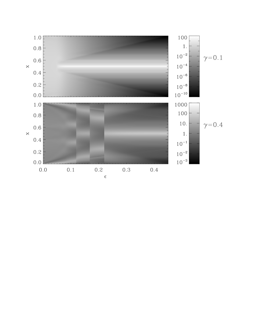
Figure 4: Plot of the asymptotic probability density $P(x,t\rightarrow\infty)$, coded in logarithmic grey levels, as a function of $\epsilon$, obtained after a numerical integration of Eq. (4) starting with a flat distribution. The top panel is for $\gamma=0.1$, and the bottom panel for $\gamma=0.4$. In both cases we used $m=0.1$ and an integration time $t=5\times 10^{4}$.

An important feature is that, for all values of $\gamma$ considered, the clusters become less defined below a critical value of $\epsilon$ (for large $\gamma$ one can always observe however the two large clusters at $x=0,1$ arising from the adsorbing boundary conditions). This point will be further addressed in section 3.

2.3 Master equation description versus Monte Carlo realizations

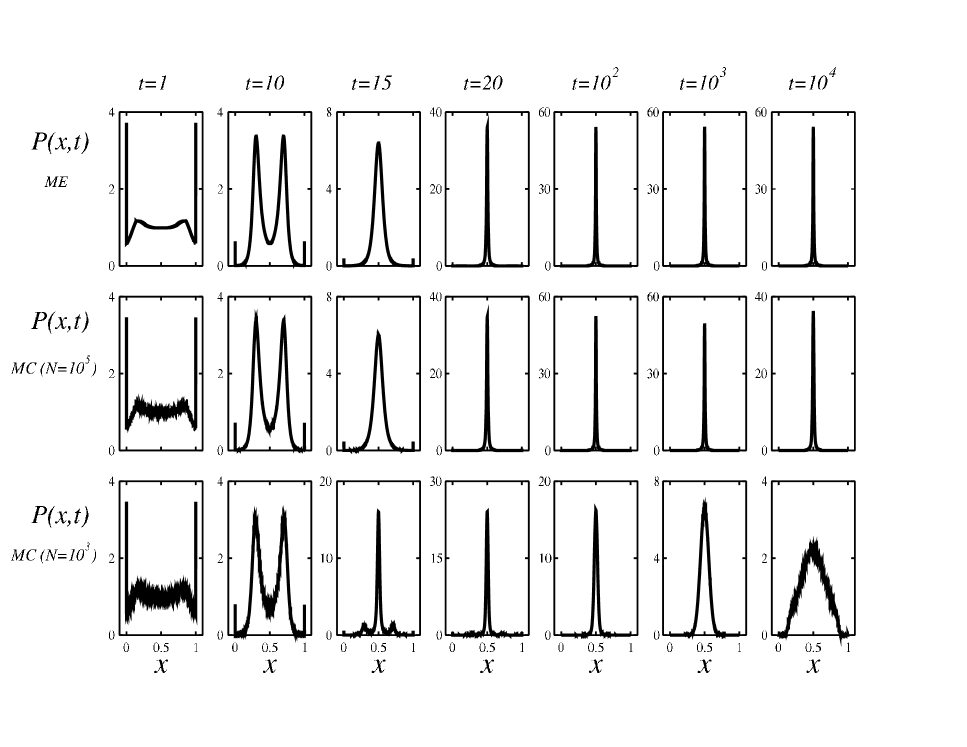
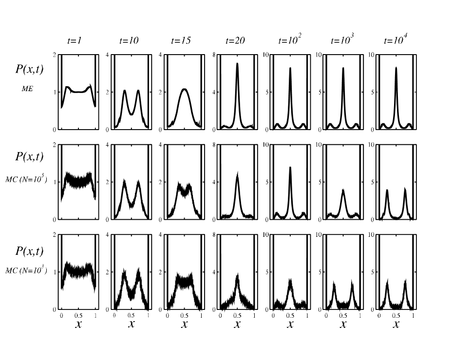
Figure 5: Probability distribution function $P(x,t)$, for intermediate time steps, from Monte-Carlo (MC) simulations (histograms binned with bin size $\Delta x=5\times 10^{-4}$) for two different system sizes $N=10^{3}$ and $N=10^{5}$, and the master equation (ME) integrations of Eq. (4) starting with a flat distribution with $\epsilon=0.28$ and $m=0.1$. The Monte Carlo distributions are an average over $10^{5}$ realizations for $N=10^{3}$ and $10^{4}$ realizations for $N=10^{5}$. The top panels present results with $\gamma=0.1$ and the bottom panels with $\gamma=0.4$.

Monte Carlo simulations with a finite number $N$ of individuals are not always faithfully represented by the solutions of the master equation, which implicitly assumes that $N\rightarrow\infty$, in addition to considering correlations between individuals only in an approximate way. In Fig. 5 we plot the time evolution of the probability coming from Monte Carlo simulations (an average of the binned opinion distribution over a large number of realizations is performed, see caption) and the results from the master equation in the case $m=0.1$ and $\epsilon=0.28$, which is close to a bifurcation from one to two big clusters in the diffusionless model (see deffuant1 for details). The top panels correspond to $\gamma=0.1$ and the bottom panels to $\gamma=0.4$. It can be seen that, although the Monte Carlo simulation and the master equation agree initially very well, they start to deviate after a time that depends on the number of individuals $N$: the larger $N$, the longer the time for which the Monte Carlo simulations are faithfully described by the master equation.

In the case $\gamma=0.1$, while the numerical solution of the master equation and Monte Carlo simulations both reach at long times a distribution with a single large maximum (large cluster) at $x=0.5$, in the Monte Carlo simulations the width of this steady distribution is larger for small particle number $N$. One can understand this by noticing that the Monte Carlo result is in fact the average over a large number of realizations, and each one of them consists on a single cluster whose location fluctuates widely (see Fig. 1). The fluctuations in the location of the center of mass of the cluster are reduced for increasing $N$ (see section 2.1), so that only the natural width of the cluster will show up for increasing $N$, the range in which the master equation description is expected to be accurate. For $\gamma=0.4$, we recover the same type of behavior already reported in our previous work concerning unbounded jumps in opinion space pineda . One can see in the bottom panel of figure 5 that while the numerical solution of the master equation tends at long times to a unimodal steady-state distribution with a single large peak (surrounded by two small ones), the Monte-Carlo simulations end up at long times in a bimodal one with two peaks. At intermediate times both types of solution agree, the larger the value of $N$ the longer the time of agreement. A similar discrepancy between the Monte-Carlo and the master equation results also appeared in our previous study concerning unbounded jumpspineda : starting from a uniform initial condition, a unimodal steady state is reached by the master equation but a bimodal distribution is the one reached instead in Monte-Carlo simulations. The point is that both distributions (the unimodal and the bimodal) are stationary solutions of the master equation, but the unimodal solution is metastable: a perturbation would take the system out of this solution towards the bimodal distribution. The perturbation needs to break the left-right symmetry (or $x\to 1-x$) of the problem which is present for a uniform initial condition. In the case of the Monte-Carlo simulations the perturbation is induced by the unavoidable finite-size fluctuations, thus explaining the discrepancies. In the case of the numerical integration of the master equation, this kind of perturbation appears if one is not careful enough and introduces, for example, round-off numerical errors that do not respect the above-mentioned symmetry.

3 Order-disorder transitions

As Fig. 4 shows, for $\epsilon$ smaller than a critical value (which depends on $m$ and $\gamma$) the probability distribution becomes blurred such that the maxima of the distributions are not evident, implying the inhibition of cluster formation and the establishment of a more homogeneous opinion distribution (although there is always some inhomogeneity close to the boundaries, specially for large $\gamma$). A similar effect can be observed with Monte-Carlo simulations under adsorbing boundary conditions and can be described in terms of an order-disorder transition: order identified with the state with well defined opinion clusters and disorder identified with the state without clusters.

To identify in a more quantitative way this order-disorder transition, we use the so-called cluster coefficient $G_{M}$ pineda ; vulpiani . Its definition starts by first dividing the opinion space $[0,1]$ in $M$ equal boxes and counting the number of individuals $l_{i}$ which, at time step $n$, have their opinion in the box $[(i-1)/M,i/M]$. The value of $M$ must not be so large that particles are artificially considered to be part of a single cluster, nor so small that statistical errors are large within one box. We choose $M=100$. One next defines an entropy $S_{M}=-\sum_{i=1}^{M}\frac{l_{i}}{N}\ln\frac{l_{i}}{N}$, and the cluster coefficient vulpiani

$$G_{M}=M^{-1}\left\langle e^{\overline{S}_{M}}\right\rangle,$$ (7)

where the over-bar denotes a temporal average in steady conditions and $\langle\cdot\rangle$ indicates an average over different realizations of the dynamics. Note that $1/M\leq G_{M}\leq 1$. Large values, $G_{M}\approx 1$, indicate that the opinions are evenly distributed along the full opinion space (a situation identified with disorder), while small values of $G_{M}$ indicate that opinions peak around a finite set of major opinion clusters (a situation identified with order).

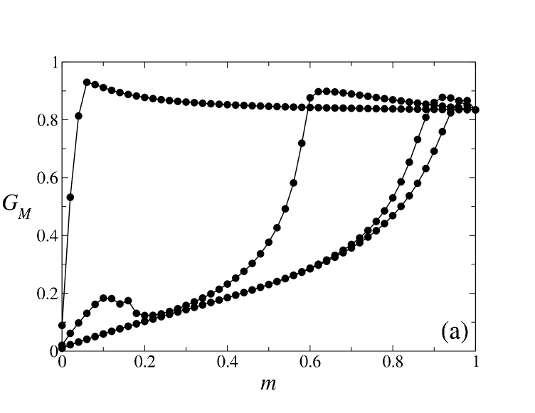
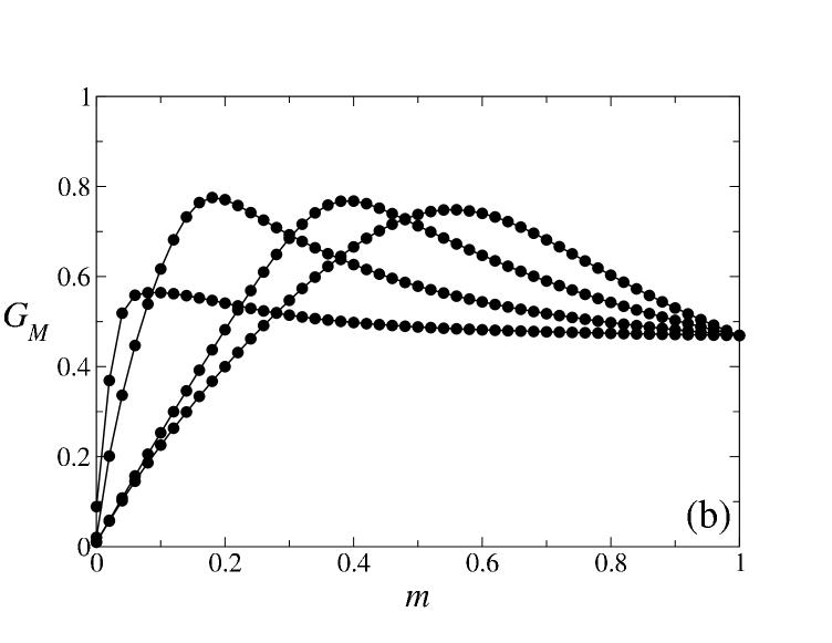
Figure 6: Opinion cluster coefficient $G_{M}$ versus $m$ for $\gamma=0.1$ (a) and $\gamma=0.4$ (b) obtained from Monte Carlo simulations with $N=10^{4}$ and adsorbing boundary conditions. The values of the confidence parameter are $\epsilon=0.05$, $0.2$, $0.4$, and $0.6$, from left to right (dots; the solid line is a guide to the eye). We will define the transition from order to disorder as the location $m_{c}$ of the absolute maximum value of $G_{M}$.

In Fig. 6($a$) we plot $G_{M}$ as a function of $m$ for $\gamma=0.1$ and different values of $\epsilon$ as obtained in the Monte Carlo simulations using adsorbing boundary conditions. For this value of $\gamma$, $G_{M}$ reaches an absolute maximum value close to $1$ (corresponding to a completely unstructured state) and then decreases monotonically. The adsorption by the extreme opinion values $0$ and $1$ prevents the formation of a fully homogeneous state (which will give $G_{M}=1$) as two opinion clusters are formed at the extrema of the opinion space, whereas the rest of the opinion space remains more or less homogeneously populated. Fig. 6($b$) shows a similar behavior in the case $\gamma=0.4$, but in this case the number of individuals whose opinion is adsorbed by the extremes is larger. Therefore, $G_{M}$ saturates farther away from its maximum possible value $1$. We will define the transition from order to disorder as the location $m_{c}$ of the absolute maximum value of $G_{M}$. In the next subsection we will explain this transition via a simple linear stability analysis that turns out to be very accurate, in particular, for small values of $\gamma$.

3.1 A linear stability analysis

Although the transition to cluster formation is a nonlinear process, one can still derive approximate analytical conditions for the existence of cluster formation as a function of the control parameters by performing a linear stability analysis of the unstructured solution of Eq. (4). This is greatly simplified if one neglects the influence of the boundaries and assumes that there are periodic boundary conditions at the ends of the interval $[0,1]$. This would be a reasonable approximation for describing the distribution far from the boundaries. We expect this approximation to be valid for not too large $\gamma$ or $\epsilon$ since, as seen for example in Fig. 4, there is not much structure near the edges of opinion space in those cases. Under periodic boundary conditions, the homogeneous configuration $P_{h}(x)=1$ is the unstructured steady solution of the master equation which results from Eqs. (4-5) without the contribution of the boundary terms:

$$\frac{\partial P(x,t)}{\partial t} = (1-m)[4\int_{|x-x_{2}|<\epsilon/2}dx_{2}P(2x-x_{2},t)P(x_{2},t)$$ (8)

$$-2P(x,t)\int_{|x-x_{2}|<\epsilon}dx_{2}P(x_{2},t)]$$

$$+m\left[\int_{x-\gamma}^{x+\gamma}\frac{dx^{\prime}}{2\gamma}P(x^{\prime}t)-P(x,t)\right].$$

To analyze the stability of the homogeneous solution $P(x)=1$ we write $P(x,t)=1+A_{q}e^{iqx+\lambda_{q}t}$, where $q$ is the wave number of the perturbation, $\lambda_{q}$ its growth rate and $A_{q}$ the amplitude. Introducing this ansatz in Eq. (8) we find the dispersion relation

$$\lambda_{q} = 4\epsilon(1-m)\left[\frac{4\sin(q\epsilon/2)}{q\epsilon}-\frac{\sin(q\epsilon)}{q\epsilon}-1\right]$$ (9)

$$+m\left[\frac{\sin(q\gamma)}{q\gamma}-1\right].$$

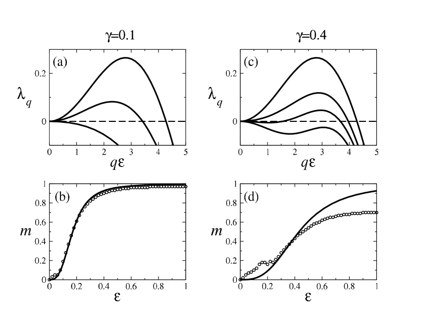
Figure 7: (a) Growth rate, equation (9), of a perturbation to the homogeneous state as a function of $q\epsilon$ for $\epsilon=0.23$, $\gamma=0.1$, and $m=0.0$, $0.4$, and $0.8$, from top to bottom. (b) Phase diagram on the plane ($\epsilon,m$) as predicted by the linear stability analysis with $\gamma=0.1$ (solid line) is compared with Monte Carlo simulations using adsorbing boundary conditions and $N=10^{4}$ (open dots). Disordered states are above the lines and ordered (clustered) ones below. (c) Growth rate as a function of $q\epsilon$ for $\epsilon=0.23$, $\gamma=0.4$, and $m=0.0$, $0.1$, $0.15$ and $0.2$, from top to bottom. (d) Phase diagram on the plane ($\epsilon,m$) as predicted by the linear stability analysis with $\gamma=0.4$ (solid line) is compared with Monte Carlo simulations using adsorbing boundary conditions and $N=10^{4}$ (open dots). Disordered states are above the lines and ordered (clustered) ones below.

We note that, for small $\gamma$ the second term, proportional to $m$, becomes $-m(\gamma q)^{2}/6$ as corresponding to the expected diffusive behavior. The top panels of Fig. 7 show this dispersion relation as a function of $q\epsilon$ for several values of $m$ with $\gamma=0.1$ and $0.4$. If there exists a wavenumber $q$ for which $\lambda_{q}>0$, then the unstructured uniform state is unstable and cluster formation will be possible. It is not possible to find closed expressions for the wavelength $q_{max}$ giving the maximum growth rate $\lambda_{q_{max}}$, or the critical values $m_{c}$ and $\epsilon_{c}$ defining the regions where the homogeneous state is stable for fixed $\gamma$, but all of this can be readily obtained numerically. Approximate analytical expressions can be obtained expanding $\lambda_{q}$ in powers of $q$:

$$\lambda_{q} = \left[-\frac{m\gamma^{2}}{6}+\frac{(1-m)}{3}\epsilon^{3}\right]q^{2}$$ (10)

$$+\frac{1}{120}\left[m\gamma^{4}-\frac{7(1-m)\epsilon^{5}}{2}\right]q^{4}+O(q^{6}).$$

In the case in which the $q^{4}$ term remains negative (which occurs if the $m\gamma^{4}$ term remains smaller than the one containing $\epsilon$), the change of sign of the $q^{2}$ term identifies $\epsilon_{c}=\left[\frac{m\gamma^{2}}{2(1-m)}\right]^{1/3}$ as the value of $\epsilon$ below which an unstructured configuration remains stable. Alternatively, for fixed $\epsilon$ we find $m_{c}=\frac{2\epsilon^{3}}{2\epsilon^{3}+\gamma^{2}}$, the critical value above which clusters will disappear. Within this approximation the expression for the fastest growing mode near the order-disorder transition is:

$$q_{max}\approx\sqrt{\frac{120}{7\epsilon_{c}^{3}-4\gamma^{2}\epsilon_{c}}}\left(\epsilon-\epsilon_{c}\right)^{1/2}.$$ (11)

We stress that all these expressions following Eq. (10) are only valid for the case in which the appearance of positive values of $\lambda_{q}$ when varying a parameter occurs first at values of $q$ close to zero, corresponding to a long-wavelength instability. As seen in Fig. 7 this is not always the case for large values of $\gamma$, for which the transitions have to be obtained numerically. In fact, we note that the change in behavior observed in the simulations from a tendency to coarsening to the establishment of a robust periodic pattern, occurring for increasing $\gamma$, seems to be correlated with the change in the character of the linear instability, from long-wavelength to finite wavelength, this last one being the one occurring in the free-will model in pineda . A more detailed discussion of the relationship between the linear dynamics and the nonlinear long-time states is however beyond the scope of this paper. Comparison of the predicted order-disorder transition with Monte Carlo simulations is performed in the bottom panels of Fig. 7. We plot the critical value $m_{c}(\epsilon)$ as obtained from the cluster coefficient $G_{M}$ (as stated before, $m_{c}$ is defined as the value at which $G_{M}$ is maximum) under adsorbing boundary conditions together with the critical lines predicted by the linear stability analysis. We see in the figure that there is a very good agreement between theory and simulations for $\gamma=0.1$, and a worse correspondence, although still qualitatively correct, for $\gamma=0.4$. Thus we can say that the arrest of cluster formation arises because the random jumps stabilize the homogeneous opinion distribution.

4 Summary and conclusions

We have studied the continuous opinion model by Deffuant et al. when one adds diffusion to the dynamics. More precisely, we have modified the evolution rules by including the probability that individuals change their opinion to another value randomly chosen inside an interval centered around the current opinion. Our aim is to include the effects of the unavoidable elements of randomness always present in human decisions. When the typical size of the random jumps is large, this model approaches a previous minimalistic model introduced by us pineda .

The final collective states depend on the system size $N$, the confidence parameter $\epsilon$ as well as on the typical size of the random jumps $\gamma$ and their probability $m$. While our numerical results consider the more natural adsorbing boundary conditions in which opinions beyond the limits of the allowed interval are set to the extreme values $0$ or $1$, some analytical calculations are carried out in the case of periodic boundary conditions, which are simpler from the mathematical point of view.

The first observation one extracts from the Monte Carlo simulations is the dispersion in the opinions within otherwise well defined opinion clusters. We believe that this effect comes closer to realistic situations in which a population splits into different groups, but the opinions of individuals within each group are not identical to each other. The detailed dynamics of those clusters depends strongly on the average size of the random jumps $\gamma$. For small values of $\gamma$, the center of mass of each cluster performs a random walk through the whole opinion space with an effective diffusion coefficient that scales with $1/N$. As a consequence, opinion clusters start to collide and merge in a coarsening process that leads to a single large cluster at very long times. For large values of $\gamma$, the mobility of clusters is reduced and several opinion clusters can appear. Thus, a small diffusion mobility favors opinion consensus.

We have derived a master equation for the probability density function $P(x,t)$ which determines the individuals density or distribution in the opinion space. Numerical integration of this equation starting from uniform initial conditions reveals that for small $\gamma$ only one opinion cluster centered around $x=0.5$ is formed for almost any value of the parameter $\epsilon$, as observed in the Monte Carlo simulations. For large $\gamma$, a sequence of bifurcations can be obtained in the opinion space. This is similar to what was found in the original Deffuant et al. model or in our previous modification pineda ; redner . We have also found that when diffusion is included, the asymptotic steady-state probability distributions reached by Monte-Carlo simulations are not always well represented by the ones obtained from the master equation dynamics starting from the same symmetric initial condition. The Monte Carlo simulations and the master equation agree initially, but start to deviate after a time that depends on the number of individuals $N$: the smaller the size, the earlier the deviation occurs. For example, it is possible to observe in the simulations bistability between one state with only one cluster (full consensus amongst the entire population) and another state with two clusters (lack of consensus or polarization in the opinions), whereas this does not appear in the master equation. We attribute this difference to the inherent fluctuations arising from the finite number of individuals of the Monte Carlo simulations. Of course, for practical applications, the number of individuals will be always finite and hence the predictions of the Monte Carlo simulations should be more relevant than those of the master equation.

An order-disorder transition to cluster formation induced by diffusion has been characterized using the so-called cluster coefficient $G_{M}$. Large $\gamma$ or $m$, or small $\epsilon$, lead to disordered (quasihomogeneous or non-clustered state). The value of $G_{M}$ in the disordered state strongly depends on the parameter $\gamma$. For small $\gamma$, $G_{M}$ reaches a maximum value close to $1$. The presence of individual’s opinions adsorbed at the extremes $0$ and $1$ does not disturb significantly the formation of an otherwise homogeneous state. For $\gamma$ large enough, the number of opinions adsorbed by the extremes increases and $G_{M}$ becomes more sensitive to $m$ and saturates far away from its maximum value $1$.

We have presented a linear stability analysis that assumes periodic boundary conditions at the ends of the $[0,1]$ interval. This analysis allows us to derive approximate conditions for opinion cluster formation as a function of the relevant parameters of the system. We have found a good qualitative agreement between the linear stability analysis and the numerical simulations using adsorbing boundary conditions and small values of $\gamma$. For large values of $\gamma$ the agreement is only qualitatively correct. Of course, the pattern selection of this model is, with diffusion and without it, intrinsically a nonlinear phenomenon and obtaining the exact critical conditions for opinion group formation remains a challenge.

Our work shows the impact of diffusion of opinions and finite-size effects on the dynamics of continuous opinion formation tt2007 . We want to emphasize that the incorporation of random perturbations in opinion dynamics induces novel and interesting phenomena and deserves to be explored in more detail in future works.

References

- (1) C. Castellano, S. Fortunato, and V. Loreto, Rev. Mod. Phys. 81, 591 (2009).
- (2) S. Galam, Eur. Phys. J. B 25, 403 (2002).
- (3) K. Sznajd-Weron and J. Sznajd, Int. J. Mod. Phys. C 11, 1157 (2000).
- (4) F. Schweitzer and J. Holyst, Eur. Phys. J. B 15, 723 (2000).
- (5) J. Lorenz, Int. J. Mod. Phys. C 18, 1819 (2007).
- (6) G. Deffuant, D. Neu, F. Amblard, and G. Weisbuch, Adv. Compl. Syst 3, 87 (2000).
- (7) G. Weisbuch, G. Deffuant, F. Amblard, and J. P. Nadal, Complexity 7, 855 (2002).
- (8) G. Weisbuch, G. Deffuant, and F. Amblard, Physica A 353, 555 (2005).
- (9) R. Hegselmann and U. Krause, J. Artif. Soc. Soc. Simul 5, 2 (2002).
- (10) B. Düring, P. Markowich, J. F. Pietschmann, and M. T. Wolfram, Proc. R. Soc. A 465, 3687 (2009).
- (11) R. Axelrod, J. Conflict Res. 41, 203 (1997).
- (12) M. Granovetter, American Journal of Sociology 83, 1420, (1978).
- (13) M. Pineda, R. Toral, and E. Hernández-García, J. Stat. Mech. P08001, (2009).
- (14) E. Ben-Naim, P. L. Krapivsky, and S. Redner, Physica D 183, 190 (2003).
- (15) A. Puglisi, V. Loreto, U. Marini Bettolo Marconi, and A. Vulpiani, Phys. Rev. E 59, 5582 (1999).
- (16) R. Toral and J. C. Tessone, Comm. Comp. Phys. 2, 177 (2007).