Fast algorithms for classical $X\to 0$ diffusion-reaction processes

Abstract

The Doi formalism treats a reaction-diffusion process as a quantum many-body problem. We use this second quantized formulation as a starting point to derive a numerical scheme for simulating $X\to 0$ reaction-diffusion processes, following a well-established time discretization procedure. In the case of a reaction zone localized in the configuration space, this formulation provides also a systematic way of designing an optimized, multiple time step algorithm, spending most of the computation time to sample the configurations where the reaction is likely to occur.

I Introduction

The reaction diffusion process $X\to 0$ with space dependent reaction rate, models a number of interesting chemical and biological situations. It models for instance the capture dynamics of a mobile ligand diffusing in a configuration space until being captured by a static receptor. This configuration space may not just be the three dimensional volume containing the molecules which participate to the reaction, but must be considered in a wider perspective. For example, in the case of a ligand bound to one end of a polymer spacer while the other end is grafted onto a surface (bridging situation 2001_Jeppesen_Marques ), the diffusive dynamics naturally takes place in a configuration space taking into account all the internal degrees of freedom of the chain, even though the reaction rate mainly depends on the position of the polymer end bearing the ligand 2004_Moreira_Marques . Biology and bio-technologies provide numerous examples of adhesion mechanisms with kinetics limited by similar reaction-diffusion dynamics 1958_Alberty_Hammes ; 1982_Chou_Zhou . The most standard immunodiagnosis assays utilize the aggregation processes based on antigen-antibody specific adhesion. It is now possible to set up finely tuned experiments with a high enough temporal resolution for the comparison of reaction kinetics with analytical or numerical predictions 1998_Chesla_Zhu ; 2008_Lee_Marques .

Polymer chemistry also offers a wide set of situations which can be advantageously modeled by a $X\to 0$ process. The cyclization reactions occurring during macromolecules synthesis are the examples 1974_Wilemski_Fixman:1 ; 1974_Wilemski_Fixman:2 . The situation can be further complicated if an external hydrodynamic flow is present, or more generally, if conservative or dissipative force fields are known to act upon the system under study 1996_Frederickson_Leibler , then calling for intensive numerical simulations 1984_Northrup_McCammon ; 1996_Pastor_Szabo .

We present in this paper a general method for finding efficient numerical simulation algorithms, using a non hermitic Hamiltonian formulation of the stochastic process introduced by Doi 1976_Doi:1 , and based on a Trotter splitting of the discrete time evolution operator. This strategy has proved successful when applied to Brownian and DPD (dissipative particle dynamics) dynamics, leading to the generation of algorithms, with controlled time-reversal or accuracy properties 2006_DeFabritiis_Coveney ; book_Frenkel_Smit ; 2003_Ricci_Ciccotti ; 2007_Thalmann_Farago .

Moreover, we suggest for this problem an original multiple time step algorithm, based on some internal state switching $A\leftrightarrow B$, which comes as a straightforward extension of the physical reaction-diffusion process. We then use a different integration time step, depending on the internal variable state, either fast or slow.

The essential strategy is to introduce fast coarse grained sampling away from the reaction zone (while keeping slow sampling near the reaction zone) in order to achieve the desired computational efficiency and accuracy. This algorithm comes as a new member in a family of optimized multiple time step algorithms, such as the RESPA 1990_Tuckerman_Berne ; 1992_Tuckerman_Martyna , and previously restricted to a fixed number of moving particles.

In this work, we restrict our approach to the case of $X\to 0$ non-interacting particles. However it can be easily extended to more general cases without difficulty. Although the formalism of Doi is not new, it is, to our knowledge, the first time that it serves as a starting point for designing a specific integration scheme for reaction-diffusion simulations.

We introduce in Section 2 the Doi formalism 1976_Doi:1 ; 1976_Doi:2 and derive the corresponding single time step algorithm. We underline in Section 3 the danger of naive incorporation of multiple integration time-steps for different regions of the configuration space, and show how to properly formulate multiple time step algorithms.

Section 4 demonstrates the validity of the whole scheme for particles diffusing on a spherical surface. The simulation time can be reduced by a large factor without noticeable artifact by choosing proper step sizes. The estimate of the expected speeding up efficiency is provided. Perspectives are outlined in our conclusive Section.

II Formalism

The standard master equation for the $X\to 0$ process is

$$\partial_{t}n(\bm{r},t)=D\nabla^{2}n(\bm{r},t)-\mu\nabla(n(\bm{r},t)\bm{f}(\bm{r},t))-S(\bm{r})n(\bm{r},t),$$ (1)

where $n(\bm{r},t)$ is the probability of finding a particle at a position $\bm{r}$, at time $t$, $S(\bm{r})$ is the space dependent reaction rate, $D$ the diffusion constant, $\mu$ the mobility coefficient, linked to $D$ by the Einstein relation $D=k_{B}T\mu$, and $\bm{f}(\bm{r})$ a space dependent, constant force field. Eq. (1) is a Fokker-Planck-Smoluchovski diffusion process, with an additional sink term accounting for particle decay. Usually, the rate $S(\bm{r})$ is a sharp function of $\bm{r}$, and represents, for instance, the very localized region in configuration space where either a binding or a chemical reaction can take place, with a precision lying in the range of the angstrom. The diffusive behavior underlying eq. (1) corresponds to an overdamped Brownian diffusion, in which the inertia of the diffusive particle plays no part.

The $X\to 0$ process does not conserve the number of particles, but is not a many-body problem, as there is no interaction affecting either the spatial motion or the reaction rate. Thus, following the idea of Doi, we introduce the second-quantized time evolution operator, that we subsequently call “Hamiltonian” by reference to standard quantum mechanics 1976_Doi:1 ; 1976_Doi:2 ; 1996_Cardy (it is also referred as a Liouvillian in related ref. 1985_Peliti ).

$$\hat{\mathcal{H}}=\int\mathrm{d}\bm{r}\bigg{[}D(\nabla a^{\dagger}(\bm{r})\cdot\nabla a(\bm{r}))-\mu(\bm{f}(\bm{r})\cdot\nabla a^{\dagger}(\bm{r}))a(\bm{r})+S(\bm{r})(a^{\dagger}(\bm{r})a(\bm{r})-a(\bm{r}))\bigg{]}.$$ (2)

In eq. (2), the first term corresponds to the Brownian diffusion term $(\hat{\mathcal{H}}_{D})$, the second one to the force induced drift term $(\hat{\mathcal{H}}_{F})$, and the last one is the space dependent reaction $X\to 0$ ($\hat{\mathcal{H}}_{R}$). The operators $a(\bm{r})$ and $a^{\dagger}(\bm{r})$ are bosonic creation and annihilation operators. Here, the use of bosonic operators means that multiple occupancy at a given position $\bm{r}$ is possible. However, in the absence of reverse reaction $0\to X$, or any other reaction creating particles X, the total number of particles present in our system can only decrease. If one starts at $t=0$ with a single particle at the origin $\bm{r}=\bm{r}_{0}$ (i.e. $n(\bm{r},\bm{r}_{0})=\delta(\bm{r}-\bm{r}_{0})$).

$$\left|{\Phi(0)}\right\rangle=a^{\dagger}(\bm{r}_{0})\left|{0}\right\rangle,$$ (3)

then the evolution operator $\exp(-\hat{\mathcal{H}}t)$ of our system, either moves or destroys this particle, and double occupancy never happens. Thus, for a single particle reaction dynamics, formally it makes no difference here whether one chooses to use bosons or fermions in eq. (2).

The connection between the second-quantized formalism and the standard formalism is made with

$$n(\bm{r},t)=\left\langle{0}\right|\exp\bigg{(}\int\mathrm{d}\bm{r}^{\prime}a(\bm{r}^{\prime})\bigg{)}a(\bm{r})\left|{\Phi(t)}\right\rangle,$$ (4)

where $\left|{\Phi(t)}\right\rangle=\exp(-\hat{\mathcal{H}}t)\left|{\Phi(0)}\right\rangle$ represents the state of the system at time $t$ 1996_Cardy . As double occupancy is precluded, one can safely replace the above expression by

$$n(\bm{r},t)=\left\langle{0}\right|a(\bm{r})\left|{\Phi(t)}\right\rangle=\left\langle{0}\right|a(\bm{r})e^{-\hat{\mathcal{H}}\,t}\left|{\Phi(0)}\right\rangle.$$ (5)

and define a propagator, for positive values of $t$

$$G(\bm{r}_{2},\bm{r}_{1};t)=\left\langle{0}\right|a(\bm{r}_{2})e^{-\hat{\mathcal{H}}\,t}a^{\dagger}(\bm{r}_{1})\left|{0}\right\rangle.$$ (6)

In eq. (2), the Hamiltonian is a sum of three non-commuting terms $\hat{\mathcal{H}}_{D}$, $\hat{\mathcal{H}}_{F}$ and $\hat{\mathcal{H}}_{R}$, and $\exp(-\hat{\mathcal{H}}t)$ is not known analytically. Following the Trotter-Strang idea, we split the evolution operators as

$$e^{-(\hat{\mathcal{H}}_{D}+\hat{\mathcal{H}}_{F}+\hat{\mathcal{H}}_{R})\,t}=\bigg{[}e^{-(\hat{\mathcal{H}}_{D}+\hat{\mathcal{H}}_{F}+\hat{\mathcal{H}}_{R})\Delta t}\bigg{]}^{t/\Delta t}\\ \simeq\bigg{[}e^{-\frac{\Delta t}{2}\hat{\mathcal{H}}_{R}}\cdot e^{-\frac{\Delta t}{2}\hat{\mathcal{H}}_{F}}\cdot e^{-\Delta t\hat{\mathcal{H}}_{D}}\cdot e^{-\frac{\Delta t}{2}\hat{\mathcal{H}}_{F}}\cdot e^{-\frac{\Delta t}{2}\hat{\mathcal{H}}_{R}}\bigg{]}^{t/\Delta t}.$$ (7)

The approximation becomes exact for $\Delta t\to 0$, and the above splitting is known to be exact up to terms of order $\Delta t^{3}$. Expression (7) has a clear algorithmic interpretation. It tells us to iterate a large number of times ($N=t/\Delta t$) a sequence of five steps, which altogether are supposed to reproduce faithfully the dynamics of the process over a time interval $\Delta t$. The error committed when doing this approximation is of order $\Delta t^{3}$ and originates from the fact that we have split the exponential of a sum of three non-commuting terms.

We now consider each one of these steps: $\exp(-\Delta t\hat{\mathcal{H}}_{R}/2)$ represents the action of the reaction term, at a fixed position, during a time interval $\Delta t/2$. Then, the survival probability of a particle initially at $\bm{r}$ is $\exp(-S(\bm{r})\Delta t/2)$, and the probability of having reacted is just $1-\exp(-S(\bm{r})\Delta t/2)$.

The term $\exp(-\Delta t\hat{\mathcal{H}}_{F}/2)$ represents a pure drift along the (constant in time) force field $\bm{f}(\bm{r})$. This is tantamount to solving the first order differential equation $\dot{\bm{r}}(t^{\prime})=\mu\bm{f}(\bm{r}(t^{\prime}))$, with initial condition $\bm{r}(t^{\prime}=0)=\bm{r}$, during a time interval $\Delta t/2$. We can check that, at the desired order of accuracy (i.e. $\Delta t^{2}$), this corresponds to a shift $\bm{r}\to\bm{r}+\mu\Delta t\tilde{\bm{f}}(\bm{r})/2$, where the pseudo force field $\tilde{\bm{f}}(\bm{r})$ is closely related to the original force field $\bm{f}(\bm{r})$, according to the Heun, or Collatz scheme (see Appendix II and ref. book_Stoer_Bulirsch ).

The term $\exp(-\Delta t\hat{\mathcal{H}}_{D})$ represents a pure Brownian diffusion in flat space, which is nothing but a Gaussian (Wiener) process with variance $2D\Delta t$.

The splitting in Eq. (7) can be cast in the algorithm presented in Table 1. At the end of this procedure, the position of the particle is

$$\bm{r}(t+\Delta t)=\bm{r}(t)+\frac{\mu\Delta t}{2}\bigg{[}\tilde{\bm{f}}(\bm{r}(t))+\tilde{\bm{f}}(\bm{r}(t)+\mu\tilde{\bm{f}}(\bm{r}(t))\Delta t/2+\Delta\bm{r}^{D})\bigg{]}+\Delta\bm{r}^{D},$$ (8)

and the survival probability is $\exp(-[S(\bm{r}(t))+S(\bm{r}(t+\Delta t))]\Delta t/2)$. If a reaction takes place, the reaction time must be set to

$$t_{R}=t+\frac{\Delta t}{2},$$ (9)

and the reaction diffusion process stops. In fact, we cannot define the reaction time more accurately than that, because any attempt to link the reaction time to one particular step in the previous algorithm would be pointless. The five steps of Algorithm I are the consequence of a formal, mathematical splitting of (7), and does not represent a consecutive sequence of events in real time.

Such an algorithm should prove successful when applied to smooth, differentiable space varying functions $S(\bm{r})$ and $\bm{f}(\bm{r})$. The accuracy of its predictions is expected, when averaged over the different Brownian paths and random reaction times $t_{R}$, to reproduce the results of the exact, continuous time process, up to and including the order $\Delta t^{2}$. These algorithms are known, in applied mathematics, as “weak order two algorithms” book_Kloeden_Platen .

III Optimization and multiple time step algorithms

The accuracy of the above numerical scheme is limited by the regularity of the functions $S(\bm{r})$ and $\bm{f}(\bm{r})$ appearing in the problem. The characteristic length scales $\Lambda_{S}$ or $\Lambda_{\bm{f}}$ upon which these functions vary set the upper bound for the discrete spatial increment $\Delta\bm{r}$, which in turn set the upper bound for the discrete time step $\Delta t$ of our dynamics.

In capture problems, it commonly happens that the reaction zone occupies only a tiny fraction of the configuration space, with a length scale $\Lambda_{S}$ of the size of the angstrom.

Using a large time step $\Delta t$ enables a fast sampling of the configuration space. However the risk of missing the reaction zone increases accordingly overlooking the possibility for the Brownian path, which is a continuous process, to come across the reaction zone and react (Fig. 1).

In practice, the time step $\Delta t$ must be chosen in order to keep the typical length step $||\bm{r}(t+\Delta t)-\bm{r}(t)||$ smaller than $\Lambda_{S}$ by a factor two or three. On the other hand, the choice of a small time step can make the computational effort unbearable if $L\gg\Lambda_{S}$, and when nothing much happens outside the reaction zone. For those reasons, it is desirable to have a multiple time step algorithm at our disposal.

A naive attempt to make a multiple time step algorithm is to divide the configuration space into two zones: a slow zone where one applies the algorithm with a small time step $\Delta t$, and a fast zone where one applies the algorithm with a larger time step ${\mathcal{F}}\Delta t$, where ${\mathcal{F}}$ is an arbitrary acceleration factor. Convenient choices for ${\mathcal{F}}$ are powers of $2$, such as ${\mathcal{F}}=8,16\ldots$, to enforce commensurability between small and fast dynamics.

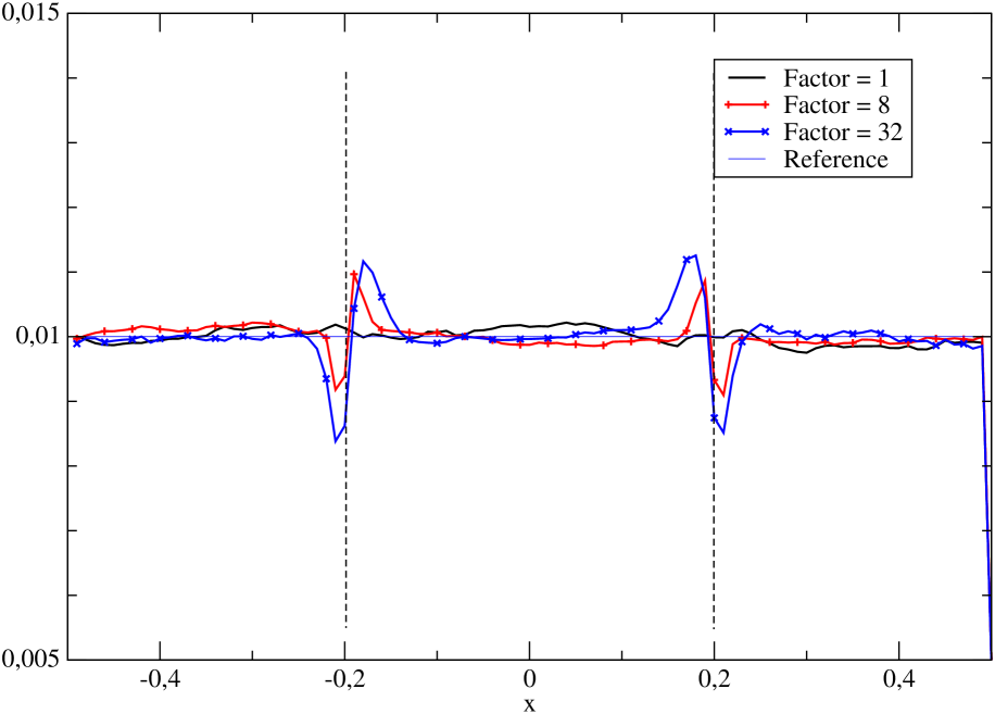
As a test case, we apply this idea to a one dimensional particle diffusing in the interval $x\in[-0.5,0.5]$ (periodic boundary conditions) with “slow” and “fast” domains and an acceleration factor ${\mathcal{F}}=8$. The large time step applies for a particle in $|x|>0.2$ and the small step for particles in $|x|<0.2$, which would correspond to a reaction zone close to $x=0$. Figure 2 shows the result of this simulation. A sharp discontinuity between fast and slow zones leads to an inhomogeneous density of particles. This artifact is located near the slow/fast boundary, with width $\sim\sqrt{2{\mathcal{F}}D\Delta t}$ given by a diffusion length, and due to a local breakdown of the detailed balance relations, where incoming particles large moves are not balanced by the reverse small moves.

In order to suppress this artifact, we propose to introduce a region, called “exchange zone”, of size $\Lambda_{w}$ where fast and slow dynamics overlap. This is achieved by adding to the diffusing particles an internal state variable, $\sigma=A$ or $B$, switching randomly between a state $A$ and a state $B$, like in a reversible chemical reaction $A\leftrightarrow B$.

The standard master equation of the process becomes:

$$\partial_{t}n_{A}(\bm{r},t) = D\nabla^{2}n_{A}(\bm{r},t)-\mu\nabla(\bm{f}(\bm{r})n_{A}(\bm{r},t))-S(\bm{r})n_{A}(\bm{r},t))$$

$$+w_{AB}(\bm{r})n_{B}(\bm{r},t)-w_{BA}(\bm{r})n_{A}(\bm{r},t);$$

$$\partial_{t}n_{B}(\bm{r},t) = D\nabla^{2}n_{B}(\bm{r},t)-\mu\nabla(\bm{f}(\bm{r})n_{B}(\bm{r},t))-S(\bm{r})n_{B}(\bm{r},t))$$ (10)

$$-w_{AB}(\bm{r})n_{B}(\bm{r},t)+w_{BA}(\bm{r})n_{A}(\bm{r},t).$$

The internal state ($\sigma=A$ or $\sigma=B$) does not alter the diffusion nor the reaction properties of the particle. $\sigma=A$ or $B$ is a hidden variable, while all the space dependent properties remain unchanged compared with eq. (1). We loosely call particle A a particle with $\sigma=A$ and particle B a particle with $\sigma=B$. In the slow diffusion limit, the equilibrium molar fraction of particles $A$ and $B$ is fixed by the exchange rates $w_{AB}(\bm{r})$ and $w_{BA}(\bm{r})$, and given by

$$x_{A}=\frac{n_{A}}{n_{A}+n_{B}} = \frac{w_{AB}(\bm{r})}{w_{AB}(\bm{r})+w_{BA}(\bm{r})};$$

$$x_{B}=\frac{n_{B}}{n_{A}+n_{B}} = \frac{w_{BA}(\bm{r})}{w_{AB}(\bm{r})+w_{BA}(\bm{r})}.$$ (11)

The exchange rates $w_{AB}(\bm{r})$ and $w_{BA}(\bm{r})$ can be arbitrarily chosen, and tailored to compromise between an strong conversion rate ($w$ must be large), and a relative smooth spatial variation ($w$ cannot vary too sharply with $\bm{r}$). We keep the size of the exchange zone $\Lambda_{w}$ two to three times larger than the spatial increment of the particles to preserve the total particle number.

The second-quantized Hamiltonian corresponding to this situation is:

$$\hat{\mathcal{H}}_{\sigma}=\hat{\mathcal{H}}_{A,R}+\hat{\mathcal{H}}_{A,D}+\hat{\mathcal{H}}_{A,F}+\hat{\mathcal{H}}_{A,Ex}+\hat{\mathcal{H}}_{B,R}+\hat{\mathcal{H}}_{B,D}+\hat{\mathcal{H}}_{B,F}+\hat{\mathcal{H}}_{B,Ex},$$ (12)

with components

$$\hat{\mathcal{H}}_{A,R} = \int\mathrm{d}\bm{r}\bigg{[}S(\bm{r})(a^{\dagger}(\bm{r})a(\bm{r})-a(\bm{r}))\bigg{]};$$ (13)

$$\hat{\mathcal{H}}_{A,D} = \int\mathrm{d}\bm{r}\bigg{[}D(\nabla a^{\dagger}(\bm{r})\cdot\nabla a(\bm{r}))\bigg{]};$$ (14)

$$\hat{\mathcal{H}}_{A,F} = \int\mathrm{d}\bm{r}\bigg{[}-\mu(\bm{f}(\bm{r})\cdot\nabla a^{\dagger}(\bm{r}))a(\bm{r})\bigg{]};$$ (15)

$$\hat{\mathcal{H}}_{A,Ex} = \int\mathrm{d}\bm{r}\bigg{[}w_{BA}(\bm{r})\bigg{(}a^{\dagger}(\bm{r})a(\bm{r})-b^{\dagger}(\bm{r})a(\bm{r})\bigg{)}\bigg{]};$$ (16)

$$\hat{\mathcal{H}}_{B,R} = \int\mathrm{d}\bm{r}\bigg{[}S(\bm{r})(b^{\dagger}(\bm{r})b(\bm{r})-b(\bm{r}))\bigg{]};$$ (17)

$$\hat{\mathcal{H}}_{B,D} = \int\mathrm{d}\bm{r}\bigg{[}D(\nabla b^{\dagger}(\bm{r})\cdot\nabla b(\bm{r}))\bigg{]};$$ (18)

$$\hat{\mathcal{H}}_{B,F} = \int\mathrm{d}\bm{r}\bigg{[}-\mu(\bm{f}(\bm{r})\cdot\nabla b^{\dagger}(\bm{r}))b(\bm{r})\bigg{]};$$ (19)

$$\hat{\mathcal{H}}_{B,Ex} = \int\mathrm{d}\bm{r}\bigg{[}w_{AB}(\bm{r})\bigg{(}b^{\dagger}(\bm{r})b(\bm{r})-a^{\dagger}(\bm{r})b(\bm{r})\bigg{)}\bigg{]}.$$ (20)

where $b,b^{\dagger}$ are bosonic creation/annihilation operators associated with particle B, and $a,a^{\dagger}$ associated with particle A. Up to this point, particles $A$ and $B$ obey the same dynamics, and one is not faster than the other. The numerical scheme originates from the splitting of $\exp(-{\mathcal{F}}\hat{\mathcal{H}}_{\sigma}\Delta t)$ as follows.

$$\exp(-{\mathcal{F}}\hat{\mathcal{H}}_{\sigma}\Delta t)=\\ \bigg{\{}e^{-\Delta t\hat{\mathcal{H}}_{B,Ex}/2}\bigg{[}e^{-\Delta t\hat{\mathcal{H}}_{B,R}/2}e^{-\Delta t\hat{\mathcal{H}}_{B,F}/2}e^{-\Delta t\hat{\mathcal{H}}_{B,D}}e^{-\Delta t\hat{\mathcal{H}}_{B,F}/2}e^{-\Delta t\hat{\mathcal{H}}_{B,R}/2}\bigg{]}e^{-\Delta t\hat{\mathcal{H}}_{B,Ex}/2}\bigg{\}}^{{\mathcal{F}}/2}\\ \times e^{-{\mathcal{F}}\Delta t\hat{\mathcal{H}}_{A,Ex}/2}\bigg{[}e^{-{\mathcal{F}}\Delta t\hat{\mathcal{H}}_{A,R}/2}e^{-{\mathcal{F}}\Delta t\hat{\mathcal{H}}_{A,F}/2}e^{-{\mathcal{F}}\Delta t\hat{\mathcal{H}}_{A,D}}e^{-{\mathcal{F}}\Delta t\hat{\mathcal{H}}_{A,F}/2}e^{-{\mathcal{F}}\Delta t\hat{\mathcal{H}}_{A,R}/2}\bigg{]}e^{-{\mathcal{F}}\Delta t\hat{\mathcal{H}}_{A,Ex}/2}\\ \times\bigg{\{}e^{-\Delta t\hat{\mathcal{H}}_{B,Ex}/2}\bigg{[}e^{-\Delta t\hat{\mathcal{H}}_{B,R}/2}e^{-\Delta t\hat{\mathcal{H}}_{B,F}/2}e^{-\Delta t\hat{\mathcal{H}}_{B,D}}e^{-\Delta t\hat{\mathcal{H}}_{B,F}/2}e^{-\Delta t\hat{\mathcal{H}}_{B,R}/2}\bigg{]}e^{-\Delta t\hat{\mathcal{H}}_{B,Ex}/2}\bigg{\}}^{{\mathcal{F}}/2}.$$ (21)

The above splitting has a straightforward algorithmic interpretation. These terms indexed by $B$ only acts on the particles whose internal state is $B$ and leave the $A$ particles unchanged with both position and internal states. The converse is true.

One recognizes three occurrences of the splitting (7), enclosed in brackets $[\cdot]$, which do not depend on the internal state of the particles, but only on the time interval (respectively $\Delta t$ or ${\mathcal{F}}\Delta t$). The splitting procedure has already been detailed in Section II. Therefore, any implementation of the single time step algorithm can be reused in the multiple time step situation, while providing also a natural checking procedure for this more complex algorithm.

The effect of $\exp(-\Delta t\hat{\mathcal{H}}_{B,Ex})$ is to exchange the internal state of $B$ particles to $A$, with a space dependent probability equal to $1-\exp(-\Delta tw_{AB}(\bm{r}))$, corresponding to a waiting time $\Delta t$. Meanwhile, particles $A$ are not affected and stay at the same position $\bm{r}$. The resulting algorithm is summed up in Table 2.

The dynamics of particles $B$ is treated with a discrete time step $\Delta t$, while the dynamics of particles $A$ is treated with a larger time step ${\mathcal{F}}\Delta t$. It is tempting to call $A$ the fast particle (or the fast state) and $B$ the slow particle (or the slow state). This linguistic shortcut must be used with care, because $A$ and $B$ particles share identical dynamic properties, and this is only the way we treat them in our discretization procedure which differs.

In practice, the exchange rates must be tailored in such a way that the reaction zone falls into a region where particles $B$ dominate. If we are confident that particles with state $A$ never wander around the reaction zone, we can safely drop the terms $\exp(-\hat{\mathcal{H}}_{A,R}\Delta t/2)$ from the algorithm. Moreover, there is a considerable room for optimizing the multiple time step algorithm, at the expense of a slightly more complex programming.

If necessary, the idea can be further extended by adding more internal states $A_{1}$,$A_{2}$, $A_{3}$…, corresponding to consecutive nested sub-domains of the configuration space. The corresponding generalization of the algorithm is straightforward.

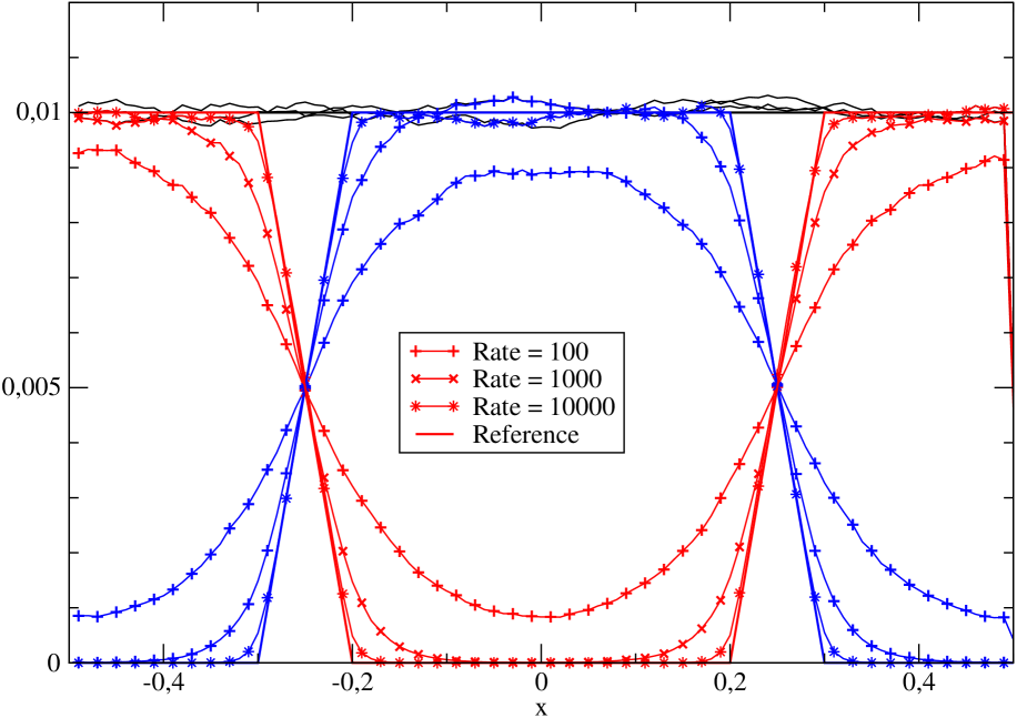
To check the relevance of the above idea, we now introduce an exchange zone for particles diffusing in one dimensional space as described earlier. The “slow” particles and “fast” particles exchange their status in a slab $0.2\leq|x|\leq 0.3$ of width $\Lambda_{w}=0.1$. The acceleration factor is kept the same ${\mathcal{F}}=8$. The average density of particles $A$ and $B$ now overlaps (see Fig. 3), and the artifact shown in Fig. 2 seems to be removed. Thus, our splitting (21) looks like an efficient strategy for keeping the advantages of a multiple time step algorithm, without suffering from appreciable unphysical features.

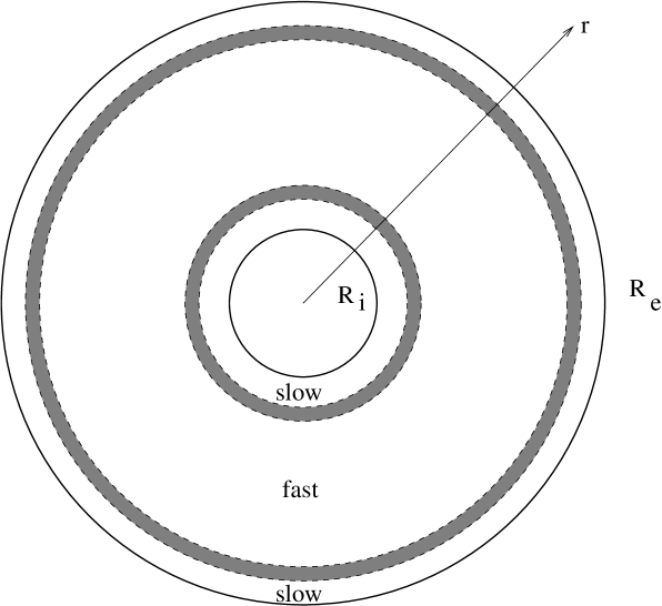
The multiple time step algorithm shows equal efficiency in higher dimensions. To demonstrate the advantages of the exchange zone in higher configurational space, we consider independent particles diffusing in a ${d_{s}}$ dimensional configuration space. Particles are reflected by a (hyper)spherical outer boundary located at distance $r=R_{e}$ from the origin and become captured when hitting an absorbing (hyper)spherical inner boundary at $r=R_{i}$, as depicted in Fig. 4. This system is a straightforward generalization of the previous unidimensional case. Despite inherent complexity, this reaction-diffusion situation remains amenable to an analytical exact solution thanks to the rotational invariance of the system. Details of the analytical solution are provided in Appendix C.

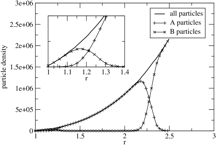
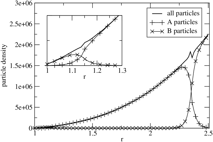
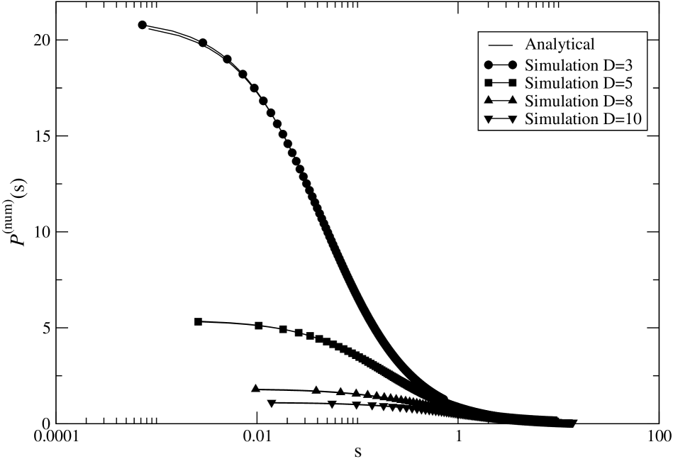
For the multiple time step procedure, we use ${\mathcal{F}}=8$ and set two exchange zones of width $\Lambda_{w}=0.15$ at the vicinity of the inner and outer walls (respectively $R_{i}=1.$ and $R_{e}\simeq 2.5$). Figure 5 shows no visible artifact in the particle distribution when the exchange zone width $\Lambda_{w}$ is kept finite, while the distribution is no longer uniform if $\Lambda_{w}=0$ as shown in Fig. 6. In Fig. 7, we compare the numerical and analytical Laplace transforms of the survival rate $\hat{P}_{D,R_{i},R_{e}}(s)$ (c.f. Appendix C), starting from a uniform particle distribution at initial time, for ${d_{s}}=3$, 5, 8 and 10. The combination of an exchange zone and internal switching state dynamics maintains a quasi-uniform distribution, while reducing the computation time by factor 2. This fits our expectation as discussed in the next section.

IV Example

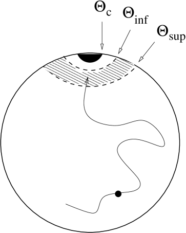
We now turn to a realistic situation to see whether our strategy keeps its promises. We consider, for example, two localized colloid carrying a ligand and many receptors, respectively, on their surfaces. These colloids combine in the form of doublet upon ligand-receptor binding. We model the rotational diffusion of colloids as random walks of a particle on a sphere. The motion of a Brownian particle evolving on a sphere is parameterized in polar coordinates $(\theta,\phi)$, with a capture zone defined by $\theta<\theta_{c}$ (Fig. 8). We performed a statistics of survival times $t_{s}$, starting from a uniform distribution of initial conditions over the sphere, until the particle encounters the capture circle $\theta=\theta_{c}$. An analytical solution of this problem, presented in 2008_Lee_Marques served as a benchmark for checking out the whole procedure.

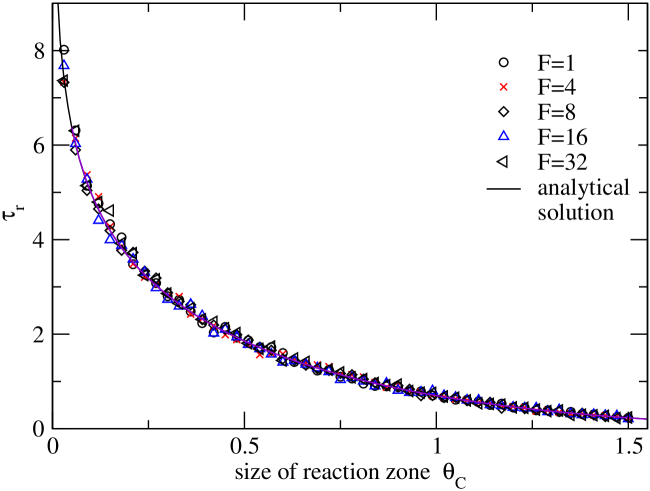
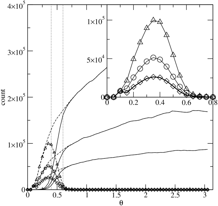
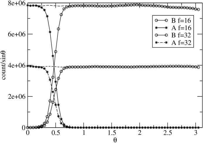
To implement the optimization procedure, we defined an exchange zone between angles $\theta_{inf}=0.4$ and $\theta_{sup}=0.6$, while the capture zone was set to $\theta_{c}=0.03$. Figure 9 shows the survival probability as a function of time for various acceleration factors ${\mathcal{F}}=4$, 8, 16 and 32 without any appreciable deviation, while the angular distribution of A and B particles is presented in Fig. 10. Meanwhile, we must check whether the multiple time step algorithm preserves the uniform distribution of positions when there is no capture (reaction off), which was achieved by counting the number of recurrences, as shown in Fig. 11.

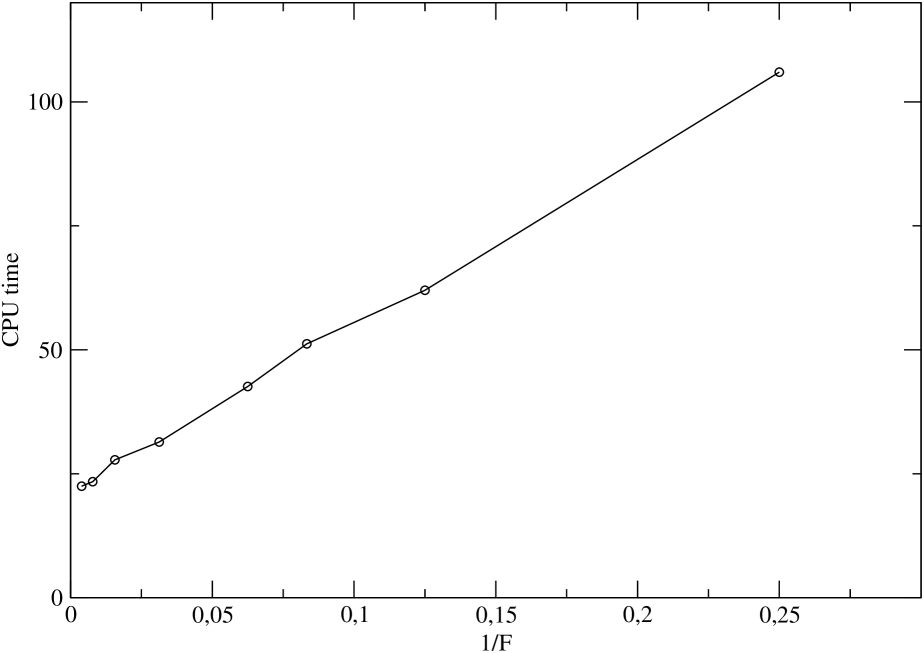
For a proper choice of ${\mathcal{F}}$, we must keep the length step smaller than the width of the exchange zone $\Lambda_{w}$. Choosing a larger ${\mathcal{F}}$ might accelerate the fast particle but requires an accordingly larger exchange zone, where the particle might spend a longer time. Hence, we observe that the CPU time is reduced by factor 6 for ${\mathcal{F}}=16$ and by 9 for ${\mathcal{F}}=32$ with $\Lambda_{w}=0.2$ and $0.4$ respectively. Corresponding CPU times are provided in Table 3. For a given ${\mathcal{F}}$, the time step of fast particle is increased by ${\mathcal{F}}$, and the corresponding length step ($\Delta\theta$) by $\sqrt{{\mathcal{F}}}$.

A rough estimate of the CPU time dependence on ${\mathcal{F}}$ can be obtained with a few approximations. Provided that the volume of the interior zone (including exchange zone) where particles are “slow” occupies a fraction $\alpha$ of the total configuration space volume $L^{d}$, and that the remaining part of the configuration space is filled with “fast” particles subject to the acceleration factor ${\mathcal{F}}$, then the time needed to sample the whole configuration space is approximately proportional to

$$\alpha+\frac{1-\alpha}{{\mathcal{F}}},$$ (22)

and the computing time reduced by a factor ${\mathcal{F}}/(1-\alpha+{\mathcal{F}}\alpha)$. In our case, with a the sphere of area $4\pi$ and an exchange zone $[0.4,0.6]$, we observe a confirmation of the expected behavior (see Fig. 12). Equation (22) also accounts fairly for the CPU time associated with the diffusion in ${d_{s}}$ dimension illustrated in Fig. 4 with a coefficient $\alpha$ comprised between 0.3 and 0.6.

If one now wishes to compare the CPU time of the multiple time step algorithm with exchange procedure (Table 1) with its single time step counterpart (Table 2), eq. (22) must be changed in

$$\bigg{[}\alpha+\frac{1-\alpha}{{\mathcal{F}}}\bigg{]}(1+\varepsilon),$$ (23)

where $\varepsilon$ accounts for the relative increase of computations associated with the exchange procedure, which depends on each specific case but should remain small in all relevant situations.

The acceleration factor ${\mathcal{F}}$ cannot exceed an upper value ${\mathcal{F}}_{max}$ dictated by the exchange zone size $\Lambda_{w}$ and slow zone size $L\alpha^{1/d}$. Thus, increasing significantly ${\mathcal{F}}$ without reintroducing spurious sampling features requires the enlargement of both exchange and slow zones, and hence does not improve so much the efficiency. The optimal strategy may consist in partitioning the configuration space into nested domains ${\mathcal{A}}_{1}$, ${\mathcal{A}}_{2}$, ${\mathcal{A}}_{3}$…associated respectively to acceleration factors $1$, ${\mathcal{F}}$, ${\mathcal{F}}^{2}$…and with geometrically increasing characteristic sizes. A well balanced partition should be such that the computer time linked to crossing each domain ${\mathcal{A}}_{i}$ remains approximately constant (a procedure reminiscent from the so-called Monte-Carlo umbrella sampling book_Frenkel_Smit or Transition Interface Sampling methods 1997_Dellago_Chandler ). In practice, values of ${\mathcal{F}}$ equal to 8 or 16 sound promising.

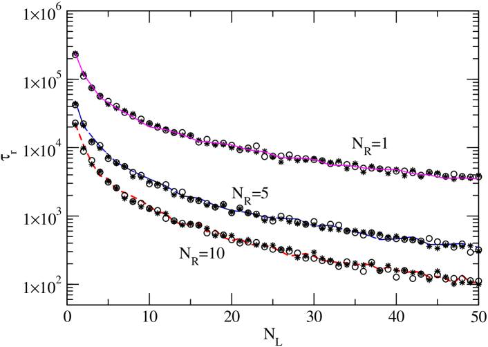
Finally, we considered the case of $N_{L}$ ligands simultaneously diffusing on a sphere covered with $N_{R}$ randomly placed receptors. There are $N_{R}$ capture zones and each capture zone is defined as angular distances from each receptor. As discussed in ref. 2008_Lee_Marques , one expects the survival probability of the ligands to decay exponentially at long times, with an inverse relaxation time proportional to the number of receptors. In Fig. 13, we compare the survival time distributions obtained with the single time step and multiple time step procedure. As shown in Fig. 13, this distribution is insensitive to the choice of the simulation procedure with the choice of a proper ${\mathcal{F}}$ (here ${\mathcal{F}}=16$).

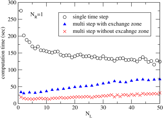
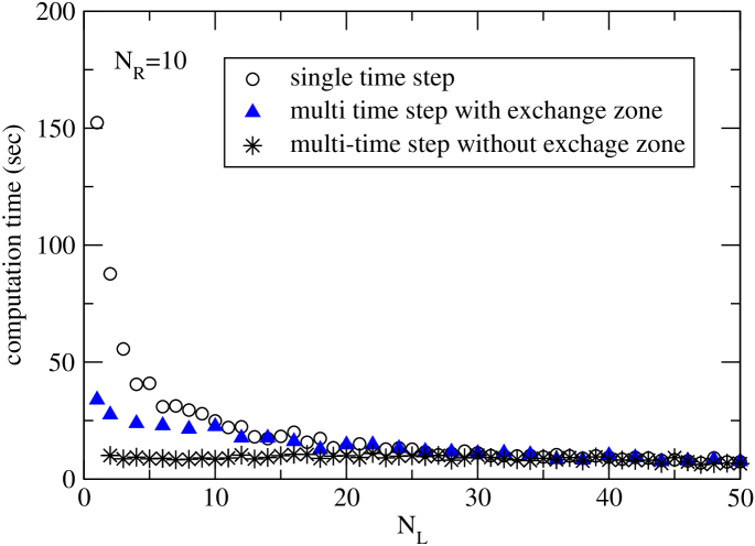
The computational time of three different procedures is compared: single time step algorithm, multiple time step algorithm with exchange zone and multiple time step algorithm without exchange zone (naive procedure). The benefits of the multiple time step algorithm decrease when the number of ligands $N_{L}$ increases. When a single receptor ($N_{R}=1$) is present on the sphere, the multiple time step algorithm performs always better than the single time step one (Fig. 14). If more receptors are present ($N_{R}=10$), the benefits of the multiple time step procedure with exchange zone are lost when the number of ligands reaches $N_{L}=20$ (Fig. 15). This is because the switching of the particle status in the exchange zone requires as many as $N_{L}\times N_{R}$ operations, which cancels out the gain from using the acceleration factor ${\mathcal{F}}\times N_{L}$ (large $\varepsilon$ in expression (23)). However, if pairwise interactions among ligands (receptors) were to be considered, the additional number of operations for particle status switching would become negligible compared with the quadratic $N_{L}^{2}$ number of operations required by the two-body interactions (small $\varepsilon$ in expression (23)). Thus, multiple time step algorithm is again clearly favorable.

V Conclusions

We presented a systematic procedure to simulate the Brownian diffusion of independent (non-interacting) and non conserved particles. Based on the second-quantized formulation of Doi, our approach uses a Trotter splitting technique and provides a weak order two algorithm for simulating the original process.

We also showed how this reaction-diffusion approach could help in finding an optimized and faithful sampling of the configuration space, in cases where the spatial resolution of the Brownian paths is not necessarily homogeneous, without showing the artifacts that other naive approaches encounter.

We tested our model on particles diffusing on a sphere and reacting at the vicinity of a pole. We were able to cut by an order of magnitude the computing time, while preserving the accuracy of the numerical scheme. When many particles diffuse simultaneously in the presence of multiple reacting zones, the efficiency of the multiple time step procedure declines for large number of particles. Although the efficiency depends on the overall algorithmic complexity of the various parts of the simulation scheme, the computation time of multiple time step algorithm is bounded by the computation time of single time step algorithm.

In the multiple time step algorithm, our trick consists in introducing an extra state variable which stochastically switches between two internal states. This procedure is certainly not restricted to the Brownian dynamics exemplified above, but might be also of interest for deterministic, or inertial Langevin dynamics. This formalism will be the natural starting point for such generalization.

Acknowledgement Author F.T. thanks KIAS for financial support during its visit. N.-K. L. acknowledges financial support by the Korea Research Foundation Grant funded by the Korean Government (MOEHRD, Basic Research Promotion Fund) (KRF-2005-204-C000024).

Appendix A Connection between second-quantized formulation and master equation

Starting from

$$n(\bm{r},t)=\left\langle{0}\right|a(\bm{r})e^{-\hat{\mathcal{H}}\,t}\left|{\Phi(0)}\right\rangle$$ (24)

one splits the evolution operator

$$e^{-\hat{\mathcal{H}}\,t}=e^{-\hat{\mathcal{H}}\,(t-t^{\prime})}\cdot e^{-\hat{\mathcal{H}}\,t^{\prime}}$$ (25)

and introduce a projector (valid only in the subspace of states with no multiple occupancy)

$$\bm{1}=\bigg{(}\left|{0}\right\rangle\left\langle{0}\right|+\int\mathrm{d}\bm{r}a^{\dagger}(\bm{r})\left|{0}\right\rangle\left\langle{0}\right|a(\bm{r})\bigg{)},$$ (26)

leading to

$$n(\bm{r},t)=\int\mathrm{d}\bm{r}^{\prime}\left\langle{0}\right|a(\bm{r})e^{-\hat{\mathcal{H}}(t-t^{\prime})}a^{\dagger}(\bm{r}^{\prime})\left|{0}\right\rangle\left\langle{0}\right|a(\bm{r}^{\prime})e^{-\hat{\mathcal{H}}t^{\prime}}\left|{\Phi(0)}\right\rangle$$ (27)

and to the well known propagator structure of the time evolution :

$$n(\bm{r},t)=\int\mathrm{d}\bm{r}^{\prime}G(\bm{r},\bm{r}^{\prime};t-t^{\prime})n(\bm{r}^{\prime},t^{\prime})$$ (28)

In the same way, the partial differential equation (1) is obtained by differentiating eq. (24) :

$$\partial_{t}n(\bm{r},t) = -\left\langle{0}\right|a(\bm{r})\hat{\mathcal{H}}e^{-\hat{\mathcal{H}}t}\left|{\Phi(0)}\right\rangle$$ (29)

$$= -\left\langle{0}\right|\hat{\mathcal{H}}a(\bm{r})e^{-\hat{\mathcal{H}}t}\left|{\Phi(0)}\right\rangle+\left\langle{0}\right|[\hat{\mathcal{H}},a(\bm{r})]e^{-\hat{\mathcal{H}}t}\left|{\Phi(0)}\right\rangle.$$

The Hamiltonian is a sum of normal ordered (creator operators on the left of annihilator operators) terms and pure annihilator terms $a(\bm{r})$, which ensures that only the second term of (29) is non zero. A standard commutator calculation leads to eq. (1).

The connection between the second-quantized formulation of the dynamics and the algorithm is done by splitting the evolution operator, such as in (7) or in eq. (21), and by introducing as many projection operators (26) as necessary between the exponentials. Each one of the $\left\langle{0}\right|a(\bm{r}_{1})e^{-\hat{\mathcal{H}}\Delta t}a^{\dagger}(\bm{r}_{2})\left|{0}\right\rangle$ has a straightforward interpretation, and corresponds to an elementary step of our algorithms I and II.

Appendix B Heun and Collatz schemes for a first order differential equation

For integrating an ordinary differential equation (o.d.e) $\dot{\bm{r}}=\bm{f}(\bm{r})$, the simplest numerical scheme is the Euler method :

$$\bm{r}(t+\Delta t)=\bm{r}(t)+\Delta t\bm{f}(\bm{r}(t)).$$ (30)

However, this scheme is known to be an “order one” integrator, which in the present situation, means that the approximated solution departs from the exact one, on a time interval $\Delta t$, by an amount of order $C\Delta t^{2}$. Clearly, this error is not acceptable as it would spoil the accuracy of the whole algorithms I and II.

Among the number of existing “order two” integrator, we propose to use either :

$$\bm{r}(t+\Delta t)=\bm{r}(t)+\frac{\Delta t}{2}\bigg{[}\bm{f}(\bm{r}(t))+\bm{f}\bigg{(}\bm{r}(t)+\Delta t\bm{f}(\bm{r}(t))\bigg{)}\bigg{]},$$ (31)

(Heun scheme), or

$$\bm{r}(t+\Delta t)=\bm{r}(t)+\Delta t\bigg{[}\bm{f}\bigg{(}\bm{r}(t)+\frac{\Delta t}{2}\bm{f}(\bm{r}(t))\bigg{)}\bigg{]},$$ (32)

(Collatz scheme) book_Stoer_Bulirsch . These schemes both require two evaluations of the function $\bm{f}(\bm{r})$ each, per time step. Once $\Delta t$ has been chosen, it is possible to give to eq. (31) and (32) a form similar to eq. (30), by defining a pseudo force field :

$$\tilde{\bm{f}}(\bm{r})=\frac{1}{2}\bigg{[}\bm{f}(\bm{r})+\bm{f}\bigg{(}\bm{r}+\bm{f}(\bm{r})\Delta t\bigg{)}\bigg{]}$$ (33)

(Heun pseudo force field), and :

$$\tilde{\bm{f}}(\bm{r})=\bm{f}\bigg{(}\bm{r}+\bm{f}(\bm{r})\frac{\Delta t}{2}\bigg{)}$$ (34)

(Collatz pseudo force field), such that :

$$\bm{r}(t+\Delta t)=\bm{r}(t)+\Delta t\,\tilde{\bm{f}}(\bm{r}(t)).$$ (35)

becomes a genuine order two integrator. We suggest to use either (34) or (35) in the steps of the algorithms associated to $e^{-\hat{\mathcal{H}}_{F}\Delta t}$.

Appendix C Diffusion and absorption in ${d_{s}}$ dimensions

To compute the survival probability between an absorbing boundary at $r=R_{i}$ and a reflecting boundary at $r=R_{e}$, we introduce the concentration of particle $c(r,t)$ at position $r$ and time $t$, obeying:

$$(\partial_{t}-\Delta)c=0,$$ (36)

with $c(R_{i},t)=0$, $\partial_{r}c(R_{e},t)=0$ and where

$$\Delta=\frac{{d_{s}}-1}{r}\frac{\mathrm{d}}{\mathrm{d}r}+\frac{\mathrm{d}^{2}}{\mathrm{d}r^{2}}$$ (37)

is the hyperspherical Laplacian in ${d_{s}}$ dimensions, discarding everything but the radial variable $r$. In this example, the diffusion constant $D$ is set to one without loss of generality. Denoting $c_{0}=c(r,0)$ the initial uniform concentration, the time Laplace transformed $\hat{c}(r,s)$ obeys

$$\Big{(}s-\frac{{d_{s}}-1}{r}\frac{\mathrm{d}}{\mathrm{d}r}-\frac{\mathrm{d}^{2}}{\mathrm{d}r^{2}}\Big{)}\hat{c}(r,s) = c_{0};$$ (38)

$$\frac{2\pi^{{d_{s}}/2}}{\Gamma({d_{s}}/2)}\int_{R_{i}}^{R_{e}}\mathrm{d}r\,r^{{d_{s}}-1}\,c_{0} = 1,$$ (39)

the solution of which can be expressed in terms of modified Bessel functions, with $\nu={d_{s}}/2-1$:

$$\hat{c}(r,s)=\frac{c_{0}}{s}\Bigg{[}1-\frac{R_{i}^{\nu}}{r^{\nu}}\frac{I_{\nu+1}(\sqrt{s}R_{e})K_{\nu}(\sqrt{s}\,r)+K_{\nu+1}(\sqrt{s}R_{e})I_{\nu}(\sqrt{s}\,r)}{I_{\nu+1}(\sqrt{s}R_{e})K_{\nu}(\sqrt{s}R_{i})+K_{\nu+1}(\sqrt{s}R_{e})I_{\nu}(\sqrt{s}R_{i})}\Bigg{]}.$$ (40)

Integrating $\hat{c}(r,s)$ over $r$ between $R_{i}$ and $R_{e}$ gives the Laplace transform $\hat{P}_{{d_{s}},R_{i},R_{e}}(s)$ of the survival rate $P_{{d_{s}},R_{i},R_{e}}(t)$:

$$\hat{P}_{{d_{s}},R_{i},R_{e}}(s)=\frac{1}{s}\Bigg{[}1+\frac{{d_{s}}}{\sqrt{s}R_{i}}\frac{1}{\bigg{[}(\frac{R_{e}}{R_{i}})^{d_{s}}-1\bigg{]}}\frac{I_{\frac{d_{s}}{2}}(\sqrt{s}R_{i})K_{\frac{d_{s}}{2}}(\sqrt{s}R_{e})-I_{\frac{d_{s}}{2}}(\sqrt{s}R_{e})K_{\frac{d_{s}}{2}}(\sqrt{s}R_{i})}{I_{\frac{d_{s}}{2}}(\sqrt{s}R_{e})K_{\frac{d_{s}}{2}-1}(\sqrt{s}R_{i})+K_{\frac{d_{s}}{2}}(\sqrt{s}R_{e})I_{\frac{d_{s}}{2}-1}(\sqrt{s}R_{i})}\Bigg{]}.$$ (41)

The survival rate $P_{{d_{s}},R_{i},R_{e}}(t)$ is a monotonically decreasing function of time $t$, giving the proportion of particles remaining after $t$, starting from a uniformly distributed random initial position in configuration space. It is related to the average survival time $\left\langle t\right\rangle$ by the simple relations:

$$\left\langle t\right\rangle=\int_{O}^{\infty}\mathrm{d}t\,P_{{d_{s}},R_{i},R_{e}}(t)=\lim_{s\to 0}\hat{P}_{{d_{s}},R_{i},R_{e}}(s).$$ (42)

The simulation provides us with a finite sample of $N$ survival times $\{t_{i}\}$, $1\leq i\leq N$. These survival times can be reordered into a monotonically increasing sequence $t_{\sigma(i)}$ by means of a suitable permutation $\sigma$ of the indexes. Such a numerical sample approximates the survival rate $P_{{d_{s}},R_{i},R_{e}}(t)$ up to statistical fluctuations of order $1/\sqrt{N}$.

In practice, this is achieved by plotting $1-i/N$ as a function of $t_{\sigma(i)}$. Alternatively this sample can be used to numerically obtain the Laplace transform of the survival rate $\hat{P}_{{d_{s}},R_{i},R_{e}}(s)$, by plotting $\hat{P}^{(\mathrm{num})}(s)$ versus $s$, as shown in Fig. 7, with $\hat{P}^{(\mathrm{num})}(s)$ defined as

$$\hat{P}^{(\mathrm{num})}(s)=\frac{1}{N}\sum_{i=1}^{N}\frac{1-\exp(-s\,t_{\sigma(i)})}{s}.$$ (43)

Figures and Tables

Algorithm I: reaction-diffusion over $\Delta t$
1. Consider the probability that a particle located at $\bm{r}(t)$ reacts during a time interval $\Delta t/2$,
given that the probability of this event is $1-\exp(-S(\bm{r}(t))\Delta t/2)$. If the particle reacts, end the
procedure and set the reaction time $t_{R}$ to $t+\Delta t/2$.
2. Shift the position of the particle by $\mu\tilde{\bm{f}}(\bm{r}(t))\Delta t/2$, as a consequence of the drift force.
3. Draw from a Gaussian distribution of variance $2D\Delta t$ a random step $\Delta\bm{r}^{D}$, and shift the
position by $\Delta\bm{r}^{D}$.
4. Shift the position by $\mu\tilde{\bm{f}}\Big{(}\bm{r}(t)+\mu\tilde{\bm{f}}(\bm{r}(t))\Delta t/2+\Delta\bm{r}^{D}\Big{)}\Delta t/2$. The particle sits now at a
position $\bm{r}(t+\Delta t)$
5. Consider the probability that a particle located at $\bm{r}(t+\Delta t)$ reacts during a time interval
$\Delta t/2$. As in step 1, if the reaction takes place, set the reaction time to $t_{R}=t+\Delta t/2$

Table 1: Algorithm for a coordinates dependent $X\to 0$ process

Algorithm II: multiple time step algorithm

1. Repeat ${\mathcal{F}}/2$ times

1.a. If the particle is $B$, consider changing its state during a time interval $\Delta t/2$, else do nothing.

1.b. If the particle is still $B$, proceed with algorithm I during the time interval $\Delta t$.

1.c.  If the particle is still $B$, consider changing its state during a time interval $\Delta t/2$, else do nothing.

2. Do once

2.a. If the particle is $A$, consider changing its state during a time interval ${\mathcal{F}}\Delta t/2$, else do nothing.

2.b. If the particle is still $A$, proceed with algorithm I during the time interval ${\mathcal{F}}\Delta t$.

2.c. If the particle is still $A$, consider changing its state during a time interval ${\mathcal{F}}\Delta t/2$, else do nothing.

3. Repeat ${\mathcal{F}}/2$ times

1.a. If the particle is $B$, consider changing its state during a time interval $\Delta t/2$, else do nothing.

1.b. If the particle is still $B$, proceed with algorithm I during the time interval $\Delta t$.

1.c.  If the particle is still $B$, consider changing its state during a time interval $\Delta t/2$, else do nothing.

Table 2: Multiple time step algorithm built on algorithm I

factor ${\mathcal{F}}$	time (s)	zone $[\theta_{inf},\theta_{sup}]$	$\Lambda_{w}$	CPU time ratio
1	299.8	$--$	$--$	1.0
4	106.0	[0.4-0.6]	0.2	0.354
8	62.0	[0.4-0.6]	0.2	0.207
12	51.2	[0.4-0.6]	0.2	0.171
16	42.6	[0.4-0.6]	0.2	0.142
16	45.1	[0.3-0.7]	0.4	0.150
32	33.5	[0.3-0.7]	0.4	0.112

Table 3: Summary of CPU times relative to the absorption of 1000 independent particles at $\theta_{c}=0.03$. Brackets indicate the limits of the exchange zone. See text for details.

FIGURE CAPTIONS

FIGURE 1.
This picture shows the principle of a multiple time step procedure for a reaction-diffusion process. Finding the small reaction well requires the step size between two consecutive spatial positions to be smaller than the size of the well. Large steps might miss the reaction well completely, and the simulated reaction rate can only be largely underestimated. However, far from the reaction zone, large steps cause no harm, and can speed up the exploration of the configuration space by a large factor. Nevertheless, the boundary between the two zone (dashed circular line) will be subject to sampling artifacts if the procedure is done without care.

FIGURE 2.
This graph presents the spurious features expected from a naive multiple time step procedure in the absence of exchange zone. When an accelerating factor ${\mathcal{F}}=8$ or ${\mathcal{F}}=32$ is introduced, two peaks appear around $x=\pm 0.2$. Their width directly depend on the length step, namely $\sqrt{2D{\mathcal{F}}\Delta t}$. This artifact comes from a local breakdown of detailed balance induced by the time discretization. The special case ${\mathcal{F}}=1$, with no acceleration, gives a control curve, constant as expected, up to statistical fluctuations.

FIGURE 3.
Particle density in the absence of reaction when dynamics is governed by the internal state exchange dynamics in one dimension. “Slow” $B$ particles occupy the central regions, and “fast” $A$ particles mainly occupy the outside of the switching zone. The flat curves show the joined $A$ and $B$ distribution, which remains constant. When the exchange rates are increased, the $A/B$ proportion tends towards its limit value (11), here a piecewise linear function. The exchange region where rates $w_{AB}(\bm{r})$ and $w_{BA}(\bm{r})$ are both non zero is the interval $[0.2,0.3]$ corresponding to an exchange zone size $\Lambda_{w}=0.1$. The acceleration factor used in this case is $\mathcal{F}=8$. The artifact in Fig. 2 is no longer visible.

FIGURE 4.
Schematic view of the ${d_{s}}$-dimensional configuration space, bounded by a reflecting outer boundary $R_{o}$ and an absorbing inner boundary $R_{i}$. Two exchange zones are indicated by grey areas limited by dashed lines.

FIGURE 5.
Repartition (density) of particles as a function of $r$, with $R_{e}\simeq 2.5$, $R_{i}=1.0$ and ${d_{s}}=5$. The exchange zone size $\Lambda_{w}$ here approaches 0.15. The inset shows an enlargement of the inner exchange zone.

FIGURE 6.
When the exchange zone is shrunk to $\Lambda_{w}=0$, under the same conditions as  Fig. 5, the unphysical heterogeneity (artefact) appears near the outer exchange zone ($r\sim 2.3$) and, to a lesser extent, near the inner exchange zone ($r\sim 1.15$ as shown on the inset of this graph).

FIGURE 7.
Comparison of the survival rate, in Laplace space, between simulations and exact result, for spatial dimensions ${d_{s}}=3,5,8$ and $10$ (see e.g. equations (41) and (43) in Appendix C). We use for the simulations an acceleration factor $\mathcal{F}=8$ and a sample size of $N=1000$ independent particles. The horizontal axis is the Laplace variable $s$ while the vertical axis has the dimension of a time. The extrapolated value as $s\to 0$ gives the average residence time $\left\langle t\right\rangle$ of the particles, and is subject to a statistical uncertainty of order $\left\langle t\right\rangle/\sqrt{N}$ (the distribution of residence times is nearly exponential).

FIGURE 8.
Pictorial view of the reaction-diffusion problem on a sphere. The exchange zone $A\leftrightarrow B$ is indicated by the shaded area. Near the capture zone, $B$ particles are subject to the small step dynamics while apart from it, $A$ particles are subject to the large step dynamics.

FIGURE 9.
The mean survival time $\left\langle\tau_{r}\right\rangle$ is calculated as a function of reaction zone size $\theta_{c}$ using different values of the acceleration ${\mathcal{F}}$ (4 to 32 indicated as symbols). The simulation results show perfect agreements with analytic results: $\left\langle\tau_{r}\right\rangle=-\ln(1-\cos(\theta_{c}))-1+\ln 2+(1-\cos(\theta_{c}))/2$, regardless of different values of ${\mathcal{F}}$. The time is measured in the unit of rotational diffusion coefficient $D_{r}$ 2008_Lee_Marques . The exchange zone $\Lambda_{w}=0.4$ is chosen to be $(\theta_{c}+0.15,\theta_{c}+0.55)$.

FIGURE 10.
Recurrence histogram of A and B particles as a function of angular positions $\theta$. Particles disappear as soon as they encounter the capture radius $\theta_{c}=0.03$ and an exchange zone is included in the region $0.4\leq\theta\leq 0.6$. Solid lines correspond to A particle with ${\mathcal{F}}=8,16,32$ from top to bottom. Symbols are for B particles with the same acceleration factors. A stationary profile is expected to be reached when particles are injected as the same rate as they are captured. The inset displays possible artifact (kinks) near the exchange zone caused by too large ${\mathcal{F}}$ values, with fast particles A able to diffuse throughout the exchange zone and to reach $\theta_{c}$. Nevertheless, the capture rate and the survival time distribution show little dependence on the choice of ${\mathcal{F}}$ (cf Fig. 9).

FIGURE 11.
Recurrence histogram of A and B particles in the interval of [$\theta$, $\theta+d\theta$] in the absence of reaction. The exchange zone is located in the interval $0.4\leq\theta\leq 0.6$. Bin counts are normalized by $\sin(\theta)$, so that uniform particle density on a sphere gives a flat histogram. The relative proportion of $A$ and $B$ particles changes smoothly across the exchange zone whereas the joined histogram remains flat. Examples are computed for ${\mathcal{F}}=16$ and ${\mathcal{F}}=32$. The total number of particles in the case of ${\mathcal{F}}=16$ is twice as large as that of ${\mathcal{F}}=32$, for given total exploration time.

FIGURE 12.
CPU time vs $1/{\mathcal{F}}$ for values of ${\mathcal{F}}$ ranging between 4 and 256. It confirms the trend CPU time $\sim\alpha+(1-\alpha)/{\mathcal{F}}$ with a fraction $\alpha\simeq 0.06$ ($\theta\simeq 0.5$), consistent with the exchange zone $[0.4,0.6]$. Note that large values of ${\mathcal{F}}$ are not only time-inefficient, but also reintroduce the unwanted spurious features, calling for an optimal compromise.

FIGURE 13.
Reaction times are evaluated by three different numerical schemes: ($\star$) a multiple-time-step procedure (${\mathcal{F}}=16$) without any exchange zone (naive approach), ($\circ$) a multiple-time-step procedure (${\mathcal{F}}=16$) with exchange zone and single time step procedure ${\mathcal{F}}=1$ (dashed line). For the given number of receptors ($N_{R}=1,5,10$), reaction times are measured as a function of the number of ligands $N_{L}$.

FIGURE 14.
Comparison of the computation times using three algorithms. In the presence of a single receptor $N_{R}=1$, the computation times for 500 reactions are measured as a function of the number of ligands $N_{L}$.

FIGURE 15.
Comparison of computational times using three algorithms. For given $N_{R}=10$, the computation time required for 500 reactions are measured as a function of $N_{L}$. See text for details.

Figure 1:

Figure 2:

Figure 3:

Figure 4:

Figure 5:

Figure 6:

Figure 7:

Figure 8:

Figure 9:

Figure 10:

Figure 11:

Figure 12:

Figure 13:

Figure 14:

Figure 15:

References

- (1) C. Jeppesen, J. Y. Wong, T.L. Kuhl, J.N. Israelachvili, N. Mullah, S. Zalipsky, and C.M. Marques, Science 293, 5529 (2001).
- (2) A.G. Moreira and C.M. Marques, J. Chem. Phys. 120, 6229 (2004).
- (3) R. A. Alberty and G.G. Hammes, J. Phys. Chem. 62, 154 (1958).
- (4) K.-C. Chou and G.-P. Zhou. J. Am. Chem. Soc. 104, 1409 (1982).
- (5) S. E. Chesla, P. Selvaraj, and C. Zhu, Biophys. J. 75, 1553 (1998).
- (6) N.-K. Lee, A. Johner, F. Thalmann, L. Cohen-Tannoudji, E. Bertrand, J. Baudry, J. Bibette, and C.M. Marques, Langmuir 24, 1296 (2008).
- (7) G. Wilemski and M. Fixman, J. Chem. Phys 60, 866 (1974).
- (8) G. Wilemski and M. Fixman, J. Chem. Phys. 60, 878 (1974).
- (9) G.H. Frederickson and L. Leibler, Macromolecules 29, 2674 (1996).
- (10) S.H. Northrup, S.A. Allison, and J.A. McCammon. J. Chem. Phys. 80, 1517, (1984).
- (11) R. W. Pastor, R. Zwanzig, and A. Szabo. J. Chem. Phys. 105, 3878 (1996).
- (12) M. Doi. J. Phys A 9, 1465 (1976).
- (13) G. de Fabritiis, M. Serrano, P. Espanol, and P.V. Coveney. Physica A 361, 429 (2006).
- (14) D. Frenkel and B. Smit.Understanding Molecular Simulations: From Algorithms to Applications (Academic Press, 2002).
- (15) A. Ricci and G. Ciccotti. Mol. Phys. 101, 1927 (2003).
- (16) F. Thalmann and J. Farago. J. Chem. Phys. 127, 124109, (2007).
- (17) M.E. Tuckerman, G.J. Martyna, and B. J. Berne. J. Chem. Phys. 93, 1287 (1990).
- (18) M. Tuckerman, B. J. Berne, and G. J. Martyna. J. Chem. Phys. 97, 1990 (1992).
- (19) Masao Doi. J. Phys. A, 9, 1479 (1976).
- (20) J. Cardy. arXiv:cond-mat/9607163, 1996.
- (21) P. Luca. J. de Phys. 46, 1469 (1985).
- (22) J. Stoer and R. Bulirsch. Text in applied mathematics 12. (Springer, 2nd edition, 1991).
- (23) Peter E. Kloeden and Eckhard Platen.Numerical Solution of Stochastic Differential Equations (Springer, 3rd edit., 1999).
- (24) C. Dellago, P.G. Bolhuis, F.S. Csajka, and D. Chandler, J. Chem. Phys. 108, 1964 (1997).