New length operator for loop quantum gravity

Abstract

An alternative expression for the length operator in loop quantum gravity is presented. The operator is background independent, symmetric, positive semidefinite, and well defined on the kinematical Hilbert space. The expression for the regularized length operator can moreover be understood both from a simple geometrical perspective as the average of a formula relating the length to area, volume and flux operators, and also consistently as the result of direct substitution of the densitized triad operator with the functional derivative operator into the regularized expression of the length. Both these derivations are discussed, and the origin of an undetermined overall factor in each case is also elucidated.

PACS numbers: 04.60.Pp, 04.60.Ds

1 Introduction

Geometrical quantities such as the length, area and volume are of great importance to general relativity (GR) as a theory of geometrodynamics. In loop quantum gravity (LQG) (for reviews on the subject, see for instance, Refs. [1, 2, 3, 4]) these operators have been realized as well-defined quantum operators on the kinematical Hilbert space, and they have been demonstrated to have discrete spectra in Refs. [5, 6, 7, 8, 9, 10]. The Bekenstein-Hawking entropy of a black hole, for instance, was computed in LQG based on the quantum area operator and the concept of isolated horizons, and the volume operator was used in constructing mathematically well-defined Hamiltonians which determine the quantum dynamics in Ref. [11]. There are also well-defined energy operators, the Arnowitt-Deser-Misner energy operator in Ref. [12] and the quasilocal energy operators in Refs. [13, 14]. Moreover, in Ref. [13] the Geroch energy operator was used to derive a rather general entropy-area relation and thus a holographic principle from loop quantum gravity.

In this work a new expression for length operator in LQG will be presented. The expression for the operator can be understood as originating from a simple geometrical formula relating the length to area, volume, and flux operators. In Euclidean 3D space, the length of an edge in a hexahedron can be expressed as a composition of the area of 2-surface, volume of region and angle between 2 surfaces in the hexahedron (see, for instance, Fig. 1). While Refs. [5, 6] have defined length operators in the framework of loop quantum gravity, a simple geometrical relationship between the length and the area, volume and angles is not articulated.

We first present a regularized length operator by transcribing the classical relation into a formula that inherits this simple geometrical composition which can be expressed directly in terms of the fundamental elements—area, volume, fluxes—of LQG. Our first method of regularization is along the lines that led to the volume operator in Ref. [9]. The final expression for the background-independent length operator contains an undetermined overall factor which arises from the process of averaging. This is also encountered in the construction of the volume operator in Ref. [9]. We use “internal” regularization (similar to the regularization of volume in Ref. [9], and so called because the regulated identity (in Sec. 3.1.1) is expressed in terms of densitized triads smeared over two surfaces within the interior of the cell). This is different from the “external” regularization introduced in Ref. [6] (the length operator therein is, without averaging, dependent on background structures). In Ref. [5] a length operator was constructed through a different strategy—substituting $e^{i}_{a}\propto\{A^{i}_{a},V\}$ in the classical length identity before regularization and quantization.

We demonstrate in a second derivation that the length operator can also be obtained by direct substitution of the densitized triad operator (similar to the method in Ref. [10]) as the functional derivative with respect to the connection into the regularized expression. An undetermined overall factor is shown to arise from the choice of a characteristic function employed in the derivation and regularization.

Although the above two routes to the length operator are rather distinct, up to the overall factor, the final expression for the background-independent quantum length operator is reassuringly identical.

2 Elements of LQG

We briefly recap the elements of LQG to establish our notations and conventions. The Hamiltonian formalism of GR is formulated on a 4-dimensional manifold $M=\mathbb{R}\times\Sigma$, with $\Sigma$ being a 3-dimensional manifold of arbitrary topology. Introducing Ashtekar-Barbero variables [15, 16], GR can be cast as a dynamical theory with $SU(2)$ ($SO(3)$ for pure GR) connection. The phase space consists of canonical pairs $(A^{i}_{a},\tilde{E}^{a}_{i})$ of fields on $\Sigma$, where $A^{i}_{a}$ is a connection 1-form which takes values in the Lie algebra $su(2)$, and $\tilde{E}^{a}_{i}$ is a vector density of weight 1. Spatial indices are denoted by $a,b,c,...$ and $i,j,k,...=1,2,3$ are internal indices. The densitized triad $\tilde{E}^{a}_{i}$ is related to the cotriad $e_{a}^{i}$ by $\tilde{E}^{a}_{i}=\frac{1}{2}\,\tilde{\epsilon}\,^{abc}\epsilon_{ijk}e^{j}_{b}e^{k}_{c}{\rm sgn}(\det(e^{i}_{a}))$, wherein $\tilde{\epsilon}\,^{abc}$ is the Levi-Cività tensor density of weight 1, and ${\rm sgn}(\det(e^{i}_{a}))$ denotes the sign of $\det(e^{i}_{a})$. The 3-metric on $\Sigma$ is expressed in terms of cotriads through $q_{ab}=e^{i}_{a}e^{j}_{b}\delta_{ij}$. The only nontrivial Poisson bracket is given by

$$\{A^{i}_{a}(x),\tilde{E}^{b}_{j}(y)\}=\kappa\beta\delta^{b}_{a}\delta^{i}_{j}\delta^{3}(x,y),$$ (1)

with $\kappa=8\pi G$, and $\beta$ is the Barbero-Immirzi parameter.

The fundamental variables in LQG are the holonomy of the connection along a curve and the flux of densitized triad through a 2-surface. Given a curve $c:[0,1]\rightarrow\Sigma$, the holonomy $h_{c}(A)$ of connection $A^{i}_{a}$ along the curve $c$ is

$$h_{c}(A)={\cal P}{\rm exp}\left(\int_{c}A\right)=1_{2}+\sum_{n=1}^{\infty}\int_{0}^{1}{\mathrm{d}}t_{1}\cdots\int_{t_{1}}^{1}{\mathrm{d}}t_{2}\cdots\int_{t_{n-1}}^{1}{\mathrm{d}}t_{n}A(c(t_{1}))\cdots A(c(t_{n})),$$ (2)

wherein ${\cal P}$ denotes the path ordering which orders the smallest path parameter to the left, $A(c(t)):=\dot{c}^{a}(t)A^{j}_{a}(c(t))\tau_{j}/2$, $\dot{c}^{a}(t)$ is the tangent vector of $c$, and $\tau_{j}=-i\sigma_{j}$ (with $\sigma_{j}$ being the Pauli matrices). The flux $\tilde{E}_{j}(S)$ of densitized triad $\tilde{E}^{a}_{j}$ through a 2-surface $S$ is explicitly

$$\tilde{E}_{j}(S)=\int_{S}n^{S}_{a}\tilde{E}^{a}_{j},$$ (3)

with $n^{S}_{a}$ being the conormal vector with respect to the surface $S$.

Another element of LQG is the notion of edges and graphs embedded in $\Sigma$ (see, for instance, [1] for a review). An edge $e$ is an equivalence class of curves $c_{e}$ which is semianalytic in all of [0, 1] . By $\gamma$ we denote a closed, piecewise analytic graph which is a set of edges that intersect at most in their end points. The collection of all end points of edges in a graph $\gamma$ is denoted by $V(\gamma)$, while the set of all edges in $\gamma$ is denoted $E(\gamma)$. In order to simplify the notation, we subdivide each edge $e$ with endpoints $v,v^{\prime}$ which are vertices of $\gamma$ into two segments $e_{1},e_{2}$ wherein $e=e_{1}\circ(e_{2})^{-1}$, with $e_{1}$ having an orientation that it is outgoing at $v$ and the orientation of $e_{2}$ is also outgoing at $v^{\prime}$. This introduces new vertices $e_{1}\cap e_{2}$ which we will call pseudovertices because they are not points of nonanalyticity of the graph. We still denote the set of these segments of $\gamma$ by $E(\gamma)$ for simplicity, but the set of true (as opposed to pseudo) vertices of $\gamma$ will be denoted as $V(\gamma)$.

To construct quantum kinematics, one has to extend the configuration space ${\cal A}$ of smooth connections to the space $\bar{\cal A}$ of distributional connections. A function $f$ on $\bar{\cal A}$ is said to be cylindrical with respect to a graph $\gamma$ iff it can be written as $f=f_{\gamma}\circ p_{\gamma}$, wherein $p_{\gamma}(A)=(h_{e_{1}}(A),..,h_{e_{n}}(A))$ and $e_{1},..,e_{n}$ are the edges of $\gamma$. Here $h_{e}(A)$ is the holonomy along $e$ evaluated at $A\in\bar{\cal A}$ and $f_{\gamma}$ is a complex-valued function on $SU(2)^{n}$. Since a function cylindrical with respect to a graph $\gamma$ is automatically cylindrical with respect to any graph bigger than $\gamma$, a cylindrical function is actually given by a whole equivalence class of functions $f_{\gamma}$. We will henceforth not distinguish between this equivalence class and one of its representatives in the set of cylindrical functions denoted by ${\rm Cyl}(\bar{\cal A})$.

Through projective techniques, $\bar{\cal A}$ is equipped with a natural, faithful, “induced” measure $\mu_{0}$, called the Ashtekar-Isham-Lewandowski measure [17, 18]. In a certain sense, this measure is the unique diffeomorphism-invariant measure on $\bar{\cal A}$ [19], and the kinematical Hilbert space is then ${\cal H}_{\mathrm{kin}}=L^{2}(\bar{\cal A},{\rm{d}}\mu_{0})$. The cylindrical function space ${\rm Cyl}(\bar{\cal A})$ is a dense subset of ${\cal H}_{\mathrm{kin}}=L^{2}(\bar{\cal A},{\rm{d}}\mu_{0})$, and cylindrical functions act by multiplication and fluxes by derivation on ${\cal H}_{\mathrm{kin}}=L^{2}(\bar{\cal A},{\rm{d}}\mu_{0})$. Given a graph $\gamma$ and a 2-surface $S$, we can change the orientations of some edges of $\gamma$ and subdivide edges of $\gamma$ into two halves at an interior point if necessary, and obtain a graph $\gamma_{\scriptscriptstyle S}$ adapted to $S$ such that the edges of $\gamma_{\scriptscriptstyle S}$ belong to the following four types [1]: (i) $e$ is up with respect to $S$ if $e\cap S=e(0)$ and $\dot{e}^{a}(0)n^{S}_{a}(e(0))>0$; (ii) $e$ is down with respect to $S$ if $e\cap S=e(0)$ and $\dot{e}^{a}(0)n^{S}_{a}(e(0))<0$; (iii) $e$ is inside with respect to $S$ if $e\cap S=e$; (iv) $e$ is outside with respect to $S$ if $e\cap S=\emptyset$. The flux operator $\hat{\tilde{E}}_{j}(S)$ acting on a function $f$ cylindrical with respect to a graph $\gamma$ adapted to $S$ is given by

$$\hat{\tilde{E}}_{j}(S)\cdot f=-\frac{i\beta\ell_{\rm p}^{2}}{4}\sum_{e\in E(\gamma)}\varrho(e,S)X^{j}_{e}\cdot f_{\gamma},$$ (4)

wherein $\ell_{\rm p}^{2}=\kappa\hbar$, $X^{j}_{e}={\rm tr}\left(\tau_{j}h_{e}(A)\frac{\partial}{\partial h_{e}(A)}\right)$ is the right invariant vector field, and $\varrho(e,S)$ takes values of $0$, $+1$ and $-1$ corresponding to whether the edge $e$ is inside/outside, up or down with respect to the surface $S$.

3 The length operator

In this section, a new length operator for LQG will be presented. To wit, let ${\cal C}$ be the set of continuous, oriented, piecewise semianalytic, parametrized, compactly supported curves embedded into $\Sigma$, wherein a curve $c\in{\cal C}$ can be parametrized by

$$c:[0,1]\rightarrow\Sigma;\quad s\mapsto c(s).$$ (5)

Then the length of the curve $c$ is given by

$$L(c) =\int_{0}^{1}{\mathrm{d}}s\sqrt{q_{ab}(c(s))\dot{c}^{a}(s)\dot{c}^{b}(s)}=\int_{0}^{1}{\mathrm{d}}s\sqrt{e^{i}_{a}(c(s))e^{j}_{b}(c(s))\delta_{ij}\dot{c}^{a}(s)\dot{c}^{b}(s)}\equiv\int_{0}^{1}{\mathrm{d}}s\sqrt{\delta_{ij}l^{i}(s)l^{j}(s)}\,,$$ (6)

wherein $q_{ab}$ is the metric of $\Sigma$, and $l^{i}(s)\equiv e^{i}_{a}(c(s))\dot{c}^{a}(s)$.

In what follows, we will regularize and quantize the length expression using two different methods following the strategies in [9] and [10]. The first method can be easily visualized geometrically, and the second has the advantage of being more direct and compact in its derivation.

3.1 The first strategy

We first define and quantize the length of a curve by adapting the framework in [9]. Our task is to regularize the expression of length in (6) into an expression which is suitable for quantization.

3.1.1 Regularization procedure for length identity

The regularization procedure involves the following ingredients. Partitioning of the curve $c$ as a composition of $N$ segments $\{c_{n}\},n\in\mathds{N},1\leq n\leq N$, i.e.,

$$c=c_{1}\circ c_{2}\circ\cdots\circ c_{n}\circ\cdots\circ c_{N},$$ (7)

wherein $\circ$ is a composition of composable curves which can be carried out with

$$c_{n}:[(n-1)\epsilon,n\epsilon]\rightarrow\Sigma;\quad s_{n}\mapsto c_{n}(s_{n}),$$ (8)

and $\epsilon=\frac{1}{N}$. The second ingredient involves a partition of the neighborhood $R_{c}$ of the curve $c$ in $\Sigma$. To do that, let us first fix global coordinates $x^{a}=(\sigma^{1},\sigma^{2},s)$ for $R_{c}$, and for each segment $c_{n}$ introduce two surfaces $S_{n}^{I},I=1,2$ intersecting in $c_{n}$ defined by $S^{1}_{n}=S^{1}_{n}(\sigma^{1}=0,\sigma^{2},s_{n})$ and $S^{2}_{n}=S^{2}_{n}(\sigma^{1},\sigma^{2}=0,s_{n})$ (with orientation induced by that of the coordinate axes). Let $n_{a}^{I}(c_{n}):=({\rm d}\sigma^{I})_{a},I=1,2$, denote the dual normal vector field of $S^{I}_{n}$. For each $c_{n}$, a close cube $\Box_{n}$ containing $c_{n}$ (determined by $S^{1}_{n}$ and $S^{2}_{n}$) gives then a partition of $R_{c_{n}}$ adapted to $c_{n}$ (see Fig. 1 (a)).

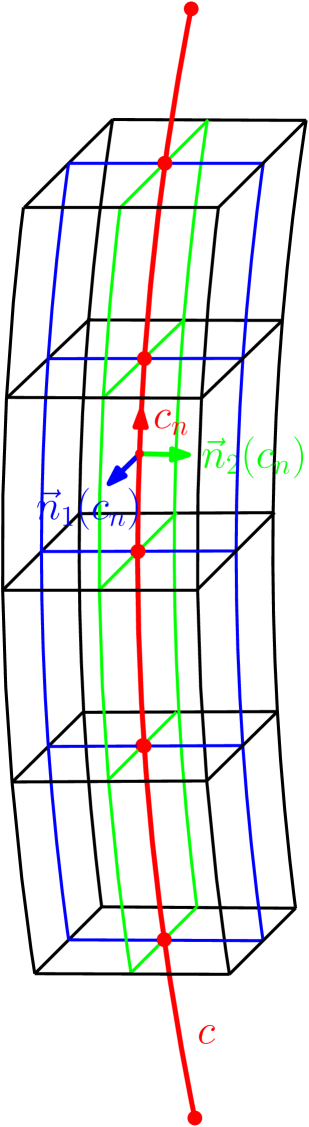
(a)

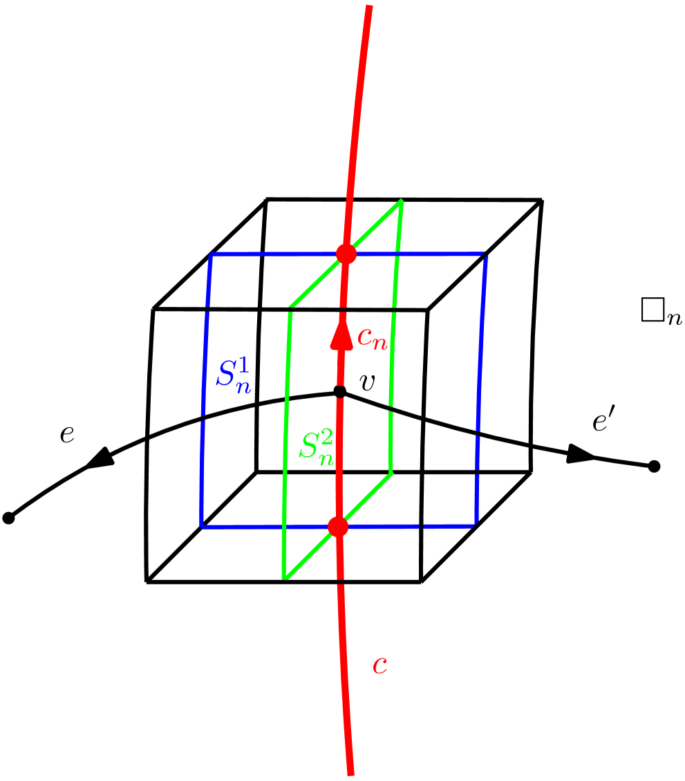
(b)

Figure 1: (a) A partition of the neighborhood $R_{c}$ of the curve $c$ in $\Sigma$ into cubes. (b) The figure illustrates the way two 2-surfaces of a partition are adapted to the curve $c_{n}$ according to conditions (i) and (ii) with the vertex $v$ at the center.

For fixed $\epsilon$, we assume that the coordinate areas $\epsilon L^{I}_{n}$ of $S^{I}_{n}$ are bounded from above by $\epsilon^{2}$ (i.e., $L^{I}_{n}<\epsilon$). Notice that

$$l^{i}(s_{n}) =\left.\frac{1}{2}\utilde{\epsilon}_{abc}\epsilon^{ijk}\tilde{E}^{b}_{j}\tilde{E}^{c}_{k}\dot{c}_{n}^{a}/\sqrt{q}\,\right|_{c_{n}(s_{n})}=\left.\frac{1}{4}\utilde{\epsilon}_{abc}\epsilon^{ijk}\tilde{E}^{b}_{j}\tilde{E}^{c}_{k}\epsilon_{IJ}\tilde{\epsilon}\,^{ade}n^{I}_{d}n_{e}^{J}/\sqrt{q}\,\right|_{c_{n}(s_{n})}=\left.\frac{1}{2}\,\epsilon_{IJ}\epsilon^{ijk}n^{I}_{b}\tilde{E}^{b}_{j}n_{c}^{J}\tilde{E}^{c}_{k}/\sqrt{q}\,\right|_{c_{n}(s_{n})},$$ (9)

wherein the identity

$$\dot{c}_{n}^{a}(s_{n})=\left.\frac{1}{2}\,\epsilon_{IJ}\tilde{\epsilon}\,^{abc}n^{I}_{b}n_{c}^{J}\right|_{c_{n}(s_{n})}.$$ (10)

has been made use of, $\utilde{\epsilon}_{abc}$ and $\epsilon_{IJ}$ are the 3D and 2D Levi-Cività tensor densities of weight $-1$, respectively. We can define the length segment via

$$L^{\epsilon}(c_{n}) :=\sqrt{\delta_{ij}l^{i}_{n,\epsilon}l^{j}_{n,\epsilon}}\,,\quad\text{with}\quad l^{i}_{n,\epsilon}=\frac{\frac{1}{2}\,\epsilon_{IJ}\epsilon^{ijk}\tilde{E}_{j}(S^{I}_{n})\tilde{E}_{k}(S^{J}_{n})}{V(\Box_{n})},$$ (11)

and $V(\Box_{n})$ is the volume of $\Box_{n}$. The expression $L^{\epsilon}(c_{n})$ yields the length $L(c)$ in (6) of the curve $c$ as

$$L(c) =\lim_{\epsilon\rightarrow 0}\sum_{n=1}^{N}L^{\epsilon}(c_{n})=\lim_{\epsilon\rightarrow 0}\sum_{n=1}^{N}\sqrt{\frac{\epsilon_{IJ}\epsilon_{KL}\tilde{E}_{j}(S^{I})\tilde{E}_{k}(S^{J})\tilde{E}_{j}(S^{K})\tilde{E}_{k}(S^{L})}{2\left[V(\Box_{n})\right]^{2}}}$$

$$=\lim_{\epsilon\rightarrow 0}\sum_{n=1}^{N}\sqrt{\frac{\tilde{E}_{j}(S^{1}_{n})\tilde{E}_{j}(S^{1}_{n})\tilde{E}_{k}(S^{2}_{n})\tilde{E}_{k}(S^{2}_{n})-\left[\tilde{E}_{j}(S^{1}_{n})\tilde{E}_{j}(S^{2}_{n})\right]^{2}}{\left[V(\Box_{n})\right]^{2}}}$$

$$=\lim_{\epsilon\rightarrow 0}\sum_{n=1}^{N}\sqrt{\frac{\left[Ar(S_{n}^{1})Ar(S_{n}^{2})\right]^{2}-\left[\tilde{E}_{j}(S^{1}_{n})\tilde{E}_{j}(S^{2}_{n})\right]^{2}}{\left[V(\Box_{n})\right]^{2}}}\,,$$ (12)

wherein $Ar(S_{n}^{I})$ is precisely the area of the surface $S^{I}_{n}$. The regulated length $L^{\epsilon}(c_{n})$ depends on the classical phase space variables through the flux, the areas of 2-surfaces and the volume of 3D region which have direct correspondence to quantum operators in LQG. Hence it is straightforward to promote $L^{\epsilon}(c_{n})$ to its quantum version $\hat{L}^{\epsilon}(c_{n})$.

A geometrical picture for the regularized expression of length in Eq. (3.1.1) can be given. Let us first recall the angle operator introduced in [20]. At $c_{n}$, the angle $\theta_{(c_{n}(s_{n}),S^{1}_{n},S^{2}_{n})}$ between $n_{a}^{1}(c_{n}(s_{n}))$ and $n_{a}^{2}(c_{n}(s_{n}))$ measured with respect to the 3D metric $q_{ab}$ is given by

$$\cos\theta_{(c_{n}(s_{n}),S^{1}_{n},S^{2}_{n})} =\frac{q^{ab}n_{a}^{1}n_{b}^{2}}{\sqrt{q^{cd}n_{c}^{1}n_{d}^{1}}\sqrt{q^{ef}n_{e}^{2}n_{f}^{2}}}\,(c(s_{n}))=\lim_{S^{1}_{n},S^{2}_{n}\rightarrow c_{n}(s_{n})}\frac{\tilde{E}_{j}(S^{1}_{n})\tilde{E}_{j}(S^{2}_{n})}{Ar(S^{1}_{n})Ar(S^{2}_{n})}.$$ (13)

With Eq. (13), the expression in Eq. (3.1.1) reduces to

$$L(c) =\lim_{\epsilon\rightarrow 0}\sum_{n=1}^{N}\sqrt{\frac{\left[Ar(S_{n}^{1})Ar(S_{n}^{2})\right]^{2}-\left[Ar(S_{n}^{1})Ar(S_{n}^{2})\cos\theta_{(c_{n}(s_{n}),S_{n}^{1},S_{n}^{2})}\right]^{2}}{\left[V(\Box_{n})\right]^{2}}}$$

$$=\lim_{\epsilon\rightarrow 0}\sum_{n=1}^{N}\frac{Ar(S_{n}^{1})Ar(S_{n}^{2})\left|\sin\theta_{(c_{n}(s_{n}),S_{n}^{1},S_{n}^{2})}\right|}{V(\Box_{n})}.$$ (14)

In our regularization procedure for the length operator, the virtue of the expression of length in (3.1.1) (or (3.1.1)) is that it is closely related to other geometric operators (area, volume, and angle) which have well-defined quantum actions. Moreover, for a rectangular hexahedron $\Box_{n}$ in flat space, $L^{\epsilon}(c_{n})$ is just the familiar expression of the length of the vertical edge $c_{n}$ of $\Box_{n}$.

The above regularization of the length is so-called internal because the regulated identity (11) is expressed in terms of triads smeared over two surfaces passing the interior of the cell and the regularization matches the internal regularization of volume in [9]. An external regularization of the length of a curve was investigated in [6].

3.1.2 Quantum length operator

The volume operator in LQG has been thoroughly discussed in Refs. [7, 9, 10], and in this work we shall focus on the volume operator in [9] ([10]). Properties of the volume operator have been investigated in [21]. The action of the volume operator measuring a region $R$ on a function $f$ cylindrical with respect to $\gamma$ is given specifically by

$$\hat{V}(R)\cdot f =\sum_{v\in V(\gamma)\cap R}\hat{V}_{v}\cdot f_{\gamma}=\ell_{\rm p}^{3}\sum_{v\in V(\gamma)\cap R}\sqrt{\left|iZ\sum_{e_{I}\cap e_{J}\cap e_{K}=v}\varsigma(e_{I},e_{J},e_{K})\epsilon_{ijk}X^{i}_{e_{I}}X^{j}_{e_{J}}X^{k}_{e_{K}}\right|}\,\cdot f_{\gamma}\,,$$ (15)

wherein $\varsigma(e_{I},e_{J},e_{K})={\rm sgn}(\det(\dot{e}_{I}(0),\dot{e}_{J}(0),\dot{e}_{K}(0)))$, and $Z$ the ambiguity factor due to regularization has been uniquely fixed as $1/(3!\times 8\times 8)$ in [22] through consistency checks of volume and triad operator regularizations. In the regulated length $L^{\epsilon}(c_{n})$ in (3.1.1) we shall need to define the inverse volume operator. The volume operator can have a large kernel, so the naive inverse volume operator $1/\hat{V}$ is not well defined, but following [6], an inverse volume operator based on the idea in [23] may be taken to be

$$\widehat{V^{-1}}:=\lim_{\epsilon\rightarrow 0}(\hat{V}^{2}+\epsilon^{2}\ell_{\rm p}^{6})^{-1}\hat{V}\,.$$ (16)

This inverse volume operator has the same properties as the volume operator in that in the limit $\lim_{\epsilon\rightarrow 0}\widehat{V^{-1}}(\Box_{n})$ acts only on the vertices of $\gamma$ of cylindrical function $f$ which are on $c_{n}$. Let us consider the partition of $R_{c}$ adapted to a graph. More precisely, we will assume that for sufficiently small $\epsilon$ the permissible partitions satisfy the following conditions: (i) $\Box_{n}$ contains at most one vertex of $\gamma$ which lies on $c_{n}$ as the interior point; (ii) if $v$ (lying on $c_{n}$) is the vertex of $\gamma$, it is the unique isolated intersection point between the union of the two 2-surfaces $S^{I}_{n}$ associated to $\Box_{n}$ and $\gamma$ (see Fig. 1 (b)). Thus $\widehat{V^{-1}}(\Box_{n})$ vanishes when $\gamma$ has no vertex contained in $\Box_{n}$. Including the nontrivial case of a vertex $v$ of $\gamma$ lying on $c_{n}$ the action of the quantum operator $\hat{l}_{n,\epsilon}^{i}$ (corresponding to $l_{n,\epsilon}^{i}$ in (11)) is then

$$\hat{l}^{i}_{n,\epsilon}\cdot f =\widehat{V(\Box_{n})^{-1}}\frac{1}{2}\epsilon_{IJ}\epsilon^{ijk}\hat{\tilde{E}}_{j}(S^{I}_{n})\hat{\tilde{E}}_{k}(S^{J}_{n})\cdot f$$

$$=-\frac{\beta^{2}\ell_{\rm p}^{4}}{32}\chi_{\scriptscriptstyle\Box_{n}}(v)\widehat{V^{-1}}_{v}\epsilon_{IJ}\epsilon^{ijk}\sum_{e(0)=v}\varrho(e,S^{I}_{n})X_{e}^{j}\sum_{e^{\prime}(0)=v}\varrho(e^{\prime},S^{J}_{n})X_{e^{\prime}}^{k}\cdot f_{\gamma}$$

$$=-\frac{\beta^{2}\ell_{\rm p}^{4}}{32}\chi_{\scriptscriptstyle\Box_{n}}(v)\widehat{V^{-1}}_{v}\sum_{e(0)=e^{\prime}(0)=v}\epsilon_{IJ}\varrho(e,S^{I}_{n})\varrho(e^{\prime},S^{J}_{n})\epsilon^{ijk}X_{e}^{j}X_{e^{\prime}}^{k}\cdot f_{\gamma}$$

$$\equiv\chi_{\scriptscriptstyle\Box_{n}}(v)\hat{l}^{i}_{v}\cdot f,$$ (17)

wherein $\chi_{\scriptscriptstyle\Box_{n}}(v)$ is the characteristic function which takes the value 1 when $v$ is contained in $\Box_{n}$ (and is zero otherwise). Also $\hat{L}^{\epsilon}(c_{n})$ (corresponding to $L^{\epsilon}(c_{n})$ in (11)) can now be defined as

$$\hat{L}^{\epsilon}(c_{n})\cdot f :=\sqrt{\hat{l}^{i}_{n,\epsilon}\left(\hat{l}^{i}_{n,\epsilon}\right)^{\dagger}}\,\cdot f=\chi_{\scriptscriptstyle\Box_{n}}(v)\sqrt{\hat{l}^{i}_{v}\left(\hat{l}^{i}_{v}\right)^{\dagger}}\,\cdot f.$$ (18)

The length operator $\hat{L}(c)$ is then

$$\hat{L}(c)=\lim_{\epsilon\rightarrow 0}\sum_{n}\hat{L}^{\epsilon}(c_{n}).$$ (19)

A choice has been made in the ordering of the noncommuting operators in the expression $\hat{l}^{i}_{v}$ wherein the volume operator has been ordered to the left, so alternatives up to these ordering ambiguities are perhaps also viable.

The action of $\hat{L}^{\epsilon}(c_{n})$ depends on the two 2-surfaces $S^{I}_{n}$ only through the properties of these surfaces at $v$. Hence, it is unchanged as we refine the partition and shrink the cell $\Box_{n}$ to $v$ and the limit is thus

$$\hat{L}(c)\cdot f=\sum_{v\in V(\gamma)\cap c}\sqrt{\hat{l}^{i}_{v}\left(\hat{l}^{i}_{v}\right)^{\dagger}}\,\cdot f_{\gamma}.$$ (20)

However, Eq. (20) carries information of our choice of partitions through the terms $\epsilon_{IJ}\varrho(e,S^{I}_{n})\varrho(e^{\prime},S^{J}_{n})$ which depend on the background structure—the coordinates choice defines the surface $S^{I}_{n}$—just as was encountered in constructing the volume operator in Ref. [9]. Hence, although the limit of $\hat{L}^{\epsilon}(c_{n})$ is well defined, it is not yet viable as a background-independent length operator. We can remove the background structure by suitably “averaging” the regularized operator over it following the strategy in [9], and obtain the average of $\epsilon_{IJ}\varrho(e,S^{I}_{n})\varrho(e^{\prime},S^{J}_{n})$ as $k_{\rm av}\varsigma(c,e,e^{\prime})$ wherein $k_{\rm av}$ is a constant, and $\varsigma(c,e,e^{\prime})$ is the orientation function which equals $+1$ $(-1)$ if the tangential directions of $c,e,e^{\prime}$ are linearly independent at the vertex $v$ and oriented positively( or negatively), or zero otherwise. The averaging yields a final well-defined background-independent LQG length operator $\hat{L}(c)$

$$\hat{L}(c)\cdot f=\sum_{v\in V(\gamma)\cap c}\sqrt{\hat{l}^{i}_{v,\rm{av}}\left(\hat{l}^{i}_{v,\rm{av}}\right)^{\dagger}}\,\cdot f_{\gamma},\qquad\text{with}\quad\hat{l}^{i}_{v,\rm{av}}=-\frac{k_{\rm av}\beta^{2}\ell_{\rm p}^{4}}{32}\,\widehat{V^{-1}}_{v}\sum_{e(0)=e^{\prime}(0)=v}\varsigma(c,e,e^{\prime})\epsilon^{ijk}X^{j}_{e}X^{k}_{e^{\prime}}.$$ (21)

3.2 The second strategy

An alternative method is to derive the length operator for LQG by adapting the technique developed in [10]. The advantage of this approach is its directness. Given a curve $c$, we may choose a coordinate system $\{x^{1},x^{2},x^{3}\}$ for the neighborhood in $\Sigma$, and let $\chi_{\scriptscriptstyle\Delta}(p,x)$ be the characteristic function in the coordinate $x$ of a cube with center $p$ spanned by three vectors ${\boldsymbol{\Delta}}_{i}=\Delta_{i}{\boldsymbol{n}}_{i}$, wherein ${\boldsymbol{n}}_{i}$ is the normal vector in the frame under consideration. The cube has coordinate volume ${\rm vol}(\Delta)=\Delta_{1}\Delta_{2}\Delta_{3}\det({\boldsymbol{n}}_{1},{\boldsymbol{n}}_{2},{\boldsymbol{n}}_{3})$, wherein $\det({\boldsymbol{n}}_{1},{\boldsymbol{n}}_{2},{\boldsymbol{n}}_{3})$ denotes the determinant of the three normal vectors in the chosen coordinates (we assume the three normal vectors to be right oriented). Explicitly,

$$\chi_{\scriptscriptstyle\Delta}(p,x)=\prod_{i=1}^{3}\theta(\frac{\Delta_{i}}{2}-|<n_{i},x-p>|)$$

with $<.,.>$ being the standard Euclidean inner product, and $\theta(y)=1$ for $y>0$ and zero otherwise. In what follows we can arbitrarily and smoothly extend the curve $c:[0,1]\rightarrow\Sigma;s\mapsto c(s)$ to $\tilde{c}:[0-\lambda,1+\lambda]\rightarrow\Sigma;t\mapsto\tilde{c}(t)$ (here $\lambda>0$) such that $\tilde{c}(t)=c(s)$ for $t=s\in[0,1]$, and denote $\tilde{c}$ by $c$ in the computations for simplicity. With $\chi_{\epsilon}(s,t)=\theta(\frac{\epsilon}{2}-|s-t|)$ wherein $s\in[0,1]$, we can then construct the smeared quantity

$$l^{i}(s,\epsilon,\Delta,\Delta^{\prime}) =\int_{-\lambda}^{1+\lambda}{\mathrm{d}}t\int_{\Sigma}{\mathrm{d}}^{3}x\int_{\Sigma}{\mathrm{d}}^{3}y\frac{\chi_{\epsilon}(s,t)}{\epsilon}\;\frac{\chi_{\scriptscriptstyle\Delta}\left(2c(s),c(t)+x\right)}{{\rm vol}(\Delta)}\frac{\chi_{\scriptscriptstyle\Delta^{\prime}}\left(3c(s),c(t)+x+y\right)}{{\rm vol}(\Delta^{\prime})}$$

$$\qquad\times\frac{1}{2\sqrt{\det(q)(x)}}\,\utilde{\epsilon}_{abc}\epsilon^{ijk}E^{b}_{j}(x)E^{c}_{k}(y)\,\dot{c}^{a}(t)\,.$$

$$\approx\frac{1}{2{\rm vol}(\Delta^{\prime})}\int_{-\lambda}^{1+\lambda}{\mathrm{d}}t\int_{\Sigma}{\mathrm{d}}^{3}x\int_{\Sigma}{\mathrm{d}}^{3}y\,\frac{\chi_{\epsilon}(s,t)}{\epsilon}\chi_{\scriptscriptstyle\Delta}\left(2c(s),c(t)+x\right)\chi_{\scriptscriptstyle\Delta^{\prime}}\left(3c(s),c(t)+x+y\right)$$

$$\qquad\times\frac{1}{V(x,\Delta)}\,\utilde{\epsilon}_{abc}\epsilon^{ijk}\dot{c}^{a}(t)E^{b}_{j}(x)E^{c}_{k}(y),$$ (22)

wherein $V(x,\Delta)$ denotes the volume of the cube $\Box^{\scriptscriptstyle\Delta}_{x}$ with center point $x$ and coordinate volume ${\rm vol}(\Delta)$, measured with respect to $q_{ab}$. The smeared quantity $l^{i}(s,\epsilon,\Delta,\Delta^{\prime})$ in (3.2) reduces to $l^{i}(s)$ in (6) when one takes the limit $\epsilon,\Delta,\Delta^{\prime}\rightarrow 0$. Hence the length of curve $c$ in (6) can be written as

$$L(c) =\lim_{\epsilon,\epsilon^{\prime}\rightarrow 0}\lim_{\Delta,\Delta^{\prime},\Delta^{\prime\prime},\Delta^{\prime\prime\prime}\rightarrow 0}\int_{0}^{1}{\mathrm{d}}s\sqrt{\delta_{ij}l^{i}(s,\epsilon,\Delta,\Delta^{\prime})l^{j}(s,\epsilon^{\prime},\Delta^{\prime\prime},\Delta^{\prime\prime\prime})}\;.$$ (23)

Again the problem of the naive inverse of the volume can be circumvented by adopting

$$\widehat{V(x,\Delta)^{-1}}\cdot f :=\lim_{\epsilon^{\prime}\rightarrow 0}\left(\frac{1}{\hat{V}(x,\Delta)^{2}+\epsilon^{\prime 2}\ell^{6}_{\rm p}}\right)\hat{V}(x,\Delta)\cdot f_{\gamma}=\lim_{\epsilon^{\prime}\rightarrow 0}\sum_{v\in V(\gamma)\cap\Box^{\scriptscriptstyle\Delta}_{x}}\left(\frac{1}{\hat{V}^{2}_{v}+\epsilon^{\prime 2}\ell^{6}_{\rm p}}\right)\hat{V}_{v}\cdot f_{\gamma}=:\sum_{v\in V(\gamma)\cap\Box^{\scriptscriptstyle\Delta}_{x}}\widehat{V^{-1}}_{v}\cdot f_{\gamma}.$$ (24)

To proceed from (3.2) to the quantum formula, we require just two steps: the first is to promote the classical inverse volume to its quantum version in (24), and the second is to replace $E^{a}_{i}$ by $\hat{\tilde{E}}^{a}_{i}(x)=-i\beta\ell_{\rm p}^{2}\delta/\delta A^{i}_{a}(x)$. The regularized expression (3.2) involves the quantum operator

$$\hat{\tilde{E}}^{a}_{i}(x,\Delta):=\frac{1}{{\rm vol}(\Delta)}\int_{\Sigma}{\mathrm{d}}^{3}y\,\chi_{\scriptscriptstyle\Delta}(x,y)\hat{\tilde{E}}^{a}_{i}(y),$$ (25)

which has a convenient action on a cylindrical function $f$. With respect to the graph $\gamma$, the result is

$$\hat{\tilde{E}}^{a}_{i}(x,\Delta)\cdot f =-\frac{i\beta\ell_{\rm p}^{2}}{2{\rm vol}(\Delta)}\sum_{e\in E(\gamma)}\int_{[0,1]}{\mathrm{d}}t\,\chi_{\scriptscriptstyle\Delta}(x,e(t))\dot{e}^{a}(t){\rm tr}\left(h_{e}(0,t)\tau_{i}h_{e}(t,1)\frac{\partial}{\partial h_{e}(0,1)}\right)\cdot f_{\gamma}.$$ (26)

wherein $h_{e}(t,t^{\prime}),t<t^{\prime}$ denotes the holonomy of $A^{i}_{a}$ along the segment $[t,t^{\prime}]\rightarrow\Sigma$ of $e$. We can next evaluate the action of $\hat{l}^{i}(s,\epsilon,\Delta,\Delta^{\prime})$ on $f$. There are two types of terms in the final result: the first type comes from only the action of two functional derivatives on $f$, while the second comes from that of one functional derivative acting on $f$ and the other acting on the trace in (26). Explicitly we have

$$\hat{l}^{i}(s,\epsilon,\Delta,\Delta^{\prime})\cdot f =-\frac{\beta^{2}\ell_{\rm p}^{4}}{8{\rm vol}(\Delta^{\prime})}\int_{-\lambda}^{1+\lambda}{\mathrm{d}}t\int_{[0,1]^{2}}{\mathrm{d}}t^{\prime}{\mathrm{d}}t^{\prime\prime}\left\{\sum_{e^{\prime},e^{\prime\prime}\in E(\gamma)}\utilde{\epsilon}_{abc}\,\dot{c}^{a}(t)\dot{e}^{\prime b}(t^{\prime})\dot{e}^{\prime\prime c}(t^{\prime\prime})\right.$$

$$\quad\qquad\times\frac{\chi_{\epsilon}(s,t)}{\epsilon}\chi_{\scriptscriptstyle\Delta}\left(2c(s),c(t)+e^{\prime}(t^{\prime})\right)\chi_{\scriptscriptstyle\Delta^{\prime}}\left(3c(s),c(t)+e^{\prime}(t^{\prime})+e^{\prime\prime}(t^{\prime\prime})\right)\widehat{V(e^{\prime}(t^{\prime}),\Delta)^{-1}}$$

$$\quad\qquad\times\epsilon^{ijk}\mathrm{tr}\left(h_{e^{\prime}}(0,t^{\prime})\tau_{j}h_{e^{\prime}}(t^{\prime},1)\frac{\partial}{\partial h_{e^{\prime}}(0,1)}\right)\mathrm{tr}\left(h_{e^{\prime\prime}}(0,t^{\prime\prime})\tau_{j}h_{e^{\prime\prime}}(t^{\prime\prime},1)\frac{\partial}{\partial h_{e^{\prime\prime}}(0,1)}\right)$$

$$\qquad{\boldsymbol{+}}\sum_{e^{\prime}\in E(\gamma)}\utilde{\epsilon}_{abc}\,\dot{c}^{a}(t)\dot{e}^{\prime b}(t^{\prime})\dot{e}^{\prime c}(t^{\prime\prime})\epsilon^{ijk}$$

$$\quad\qquad\times\chi_{\epsilon}(c(s),c(t))\chi_{\scriptscriptstyle\Delta}\left(2c(s),c(t)+e^{\prime}(t^{\prime})\right)\chi_{\scriptscriptstyle\Delta^{\prime}}\left(3c(s),c(t)+e^{\prime}(t^{\prime})+e^{\prime}(t^{\prime\prime})\right)\widehat{V(e^{\prime}(t^{\prime}),\Delta)^{-1}}$$

$$\quad\qquad\times\left[\theta(t^{\prime\prime}-t^{\prime})\mathrm{tr}\left(h_{e^{\prime}}(0,t^{\prime})\tau_{j}h_{e^{\prime}}(t^{\prime},t^{\prime\prime})\tau_{k}h_{e^{\prime}}(t^{\prime\prime},1)\frac{\partial}{\partial h_{e^{\prime}}(0,1)}\right)\right.$$

$$\quad\qquad\quad\left.+\left.\theta(t^{\prime}-t^{\prime\prime})\mathrm{tr}\left(h_{e^{\prime}}(0,t^{\prime\prime})\tau_{j}h_{e^{\prime}}(t^{\prime\prime},t^{\prime})\tau_{k}h_{e^{\prime}}(t^{\prime},1)\frac{\partial}{\partial h_{e^{\prime}}(0,1)}\right)\right]\right\}\cdot f_{\gamma}$$

$$\equiv-\frac{\beta^{2}\ell_{\rm p}^{4}}{8{\rm vol}(\Delta^{\prime})}\int_{-\lambda}^{1+\lambda}{\mathrm{d}}t\int_{[0,1]^{2}}{\mathrm{d}}t^{\prime}{\mathrm{d}}t^{\prime\prime}$$

$$\quad\times\left\{\sum_{e^{\prime},e^{\prime\prime}\in E(\gamma)}\utilde{\epsilon}_{abc}\,\dot{c}^{a}(t)\dot{e}^{\prime b}(t^{\prime})\dot{e}^{\prime\prime c}(t^{\prime\prime})\widehat{V(e^{\prime}(t^{\prime}),\Delta)^{-1}}\hat{O}^{i}_{ce^{\prime}e^{\prime\prime}}(t,t^{\prime},t^{\prime\prime})\right.$$

$$\qquad\qquad\qquad\qquad\times\frac{\chi_{\epsilon}(s,t)}{\epsilon}\chi_{\scriptscriptstyle\Delta}\left(2c(s),c(t)+e^{\prime}(t^{\prime})\right)\chi_{\scriptscriptstyle\Delta^{\prime}}\left(3c(s),c(t)+e^{\prime}(t^{\prime})+e^{\prime\prime}(t^{\prime\prime})\right)$$

$$\qquad\quad{\boldsymbol{+}}\sum_{e^{\prime}\in E(\gamma)}\utilde{\epsilon}_{abc}\,\dot{c}^{a}(t)\dot{e}^{\prime b}(t^{\prime})\dot{e}^{\prime c}(t^{\prime\prime})\widehat{V(e^{\prime}(t^{\prime}),\Delta)^{-1}}\hat{O^{\prime}}^{i}_{ce^{\prime}e^{\prime}}(t,t^{\prime},t^{\prime\prime})$$

$$\qquad\qquad\qquad\qquad\left.\times\frac{\chi_{\epsilon}(s,t)}{\epsilon}\chi_{\scriptscriptstyle\Delta}\left(2c(s),c(t)+e^{\prime}(t^{\prime})\right)\chi_{\scriptscriptstyle\Delta^{\prime}}\left(3c(s),c(t)+e^{\prime}(t^{\prime})+e^{\prime}(t^{\prime\prime})\right)\right\}\cdot f_{\gamma}.$$ (27)

Given a triple $(c,e^{\prime},e^{\prime\prime})$ consisting of a curve $c$ and two edges $e^{\prime},e^{\prime\prime}$ in $E(\gamma)$ (which contains the case $e^{\prime}=e^{\prime\prime}$), we may consider the vector valued function

$$z_{c,e^{\prime},e^{\prime\prime}}(t,t^{\prime},t^{\prime\prime}):=c(t)+e^{\prime}(t^{\prime})+e^{\prime\prime}(t^{\prime\prime}).$$ (28)

Its Jacobian

$$\det\left(\frac{\partial\left(z^{1}_{ce^{\prime}e^{\prime\prime}},z^{2}_{ce^{\prime}e^{\prime\prime}},z^{3}_{ce^{\prime}e^{\prime\prime}}\right)(t,t^{\prime},t^{\prime\prime})}{\partial(t,t^{\prime},t^{\prime})}\right)=\,\utilde{\epsilon}_{abc}\,\dot{c}^{a}(t)\dot{e}^{\prime b}(t^{\prime})\dot{e}^{\prime\prime c}(t^{\prime\prime})$$ (29)

is precisely the factor that appears in all the integrals in (3.2). This is also the motivation for introducing the special characteristic function $\chi_{\scriptscriptstyle\Delta^{\prime}}\left(3c(s),c(t)+x+y\right)$ in (3.2).

Let us first take the limit $\Delta^{\prime}\rightarrow 0$. The integrand in (3.2) vanishes unless $c(s)$ is a vertex $v=e^{\prime}\cap e^{\prime\prime}$ of the graph $\gamma$ in the limit. On the other hand, in order to make the determinant nonvanishing at $c(s)$, the two edges $e^{\prime},e^{\prime\prime}$ and the curve $c$ must be distinct from one another. Hence, the second term in (3.2), which involves only summation over $e^{\prime}(=e^{\prime\prime})$, vanishes. Now by letting $\Delta^{\prime}$ be sufficiently small, the condition $\chi_{\scriptscriptstyle\Delta^{\prime}}\left(c(s),z_{ce^{\prime}e^{\prime\prime}}\right)=1$ implies $\chi_{\scriptscriptstyle\Delta}\left(2c(s),c(t)+e^{\prime}(t^{\prime})\right)=\chi_{\epsilon}(s,t)=1$, so that we can pull the remaining characteristic functions $\chi_{\scriptscriptstyle\Delta}\left(2c(s),c(t)+e^{\prime}(t^{\prime})\right)$ and $\chi_{\epsilon}(s,t)$ out of the integral by replacing them with $\chi_{\scriptscriptstyle\Delta}(c(s),v)=1$ and $\chi_{\epsilon}(s,c^{-1}(v))$, respectively. For the case $c\cap e^{\prime}\cap e^{\prime\prime}=c(s)=v$ is an outgoing point (i.e. the parameters of the edges $e^{\prime}$ and $e^{\prime\prime}$ in our notation described in Sec. 2 take the value 0), we can also replace the operators $\widehat{V(e^{\prime}(t^{\prime}),\Delta)^{-1}}$ and $\hat{O}^{i}_{ce^{\prime}e^{\prime\prime}}(t,t^{\prime},t^{\prime\prime})$ by $\widehat{V(v,\Delta)^{-1}}$ and $\hat{O}^{i}_{ce^{\prime}e^{\prime\prime}}(c^{-1}(v),0,0)$. Hence (3.2) reduces to

$$\lim_{\Delta^{\prime}\rightarrow 0}\hat{l}^{i}(s,\epsilon,\Delta,\Delta^{\prime})\cdot f =-\frac{\beta^{2}\ell_{\rm p}^{4}}{8}\sum_{v\in V(\gamma)\cap c}\frac{\chi_{\epsilon}(s,c^{-1}(v))}{\epsilon}\,\widehat{V(v,\Delta)^{-1}}$$

$$\qquad\qquad\times\sum_{e^{\prime}\cap e^{\prime\prime}=v}\;\hat{O}_{ce^{\prime}e^{\prime\prime}}(c^{-1}(v),0,0)\int_{-\lambda}^{1+\lambda}{\mathrm{d}}t\int_{[0,1]^{2}}{\mathrm{d}}t^{\prime}{\mathrm{d}}t^{\prime\prime}\delta^{3}(c(s),x)\det\left(\frac{\partial(z^{a}_{ce^{\prime}e^{\prime\prime}})}{\partial(t,t^{\prime},t^{\prime\prime})}\right)\cdot f_{\gamma}$$

$$=-\frac{\beta^{2}\ell_{\rm p}^{4}}{8}\sum_{v\in V(\gamma)\cap c}\frac{\chi_{\epsilon}(s,c^{-1}(v))}{\epsilon}\,\widehat{V(v,\Delta)^{-1}}\sum_{e^{\prime}\cap e^{\prime\prime}=v}\;\hat{O}^{i}_{ce^{\prime}e^{\prime\prime}}(c^{-1}(v),0,0)\varsigma(c,e^{\prime},e^{\prime\prime})\int{\rm d}^{3}z\delta^{3}(c(s),z)\cdot f_{\gamma}$$

$$=-\frac{\beta^{2}\ell_{\rm p}^{4}}{8\times 4}\sum_{v\in V(\gamma)\cap c}\frac{\chi_{\epsilon}(s,c^{-1}(v))}{\epsilon}\,\widehat{V(v,\Delta)^{-1}}\sum_{e^{\prime}\cap e^{\prime\prime}=v}\;\varsigma(c,e^{\prime},e^{\prime\prime})\hat{O}^{i}_{ce^{\prime}e^{\prime\prime}}(c^{-1}(v),0,0)\cdot f_{\gamma},$$ (30)

wherein $\varsigma(c,e^{\prime},e^{\prime\prime}):={\rm sgn}(\det(\dot{c}(c^{-1}(v)),\dot{e}^{\prime}(0),\dot{e}^{\prime\prime}(0))$, $\hat{O}^{i}_{ce^{\prime}e^{\prime\prime}}(c^{-1}(v),0,0):=\epsilon^{ijk}X^{j}_{e^{\prime}}X^{k}_{e^{\prime\prime}}$, and the factor $1/4$ came from the fact that the integral just equals $\int_{-\lambda}^{1+\lambda}{\mathrm{d}}t\int_{[0,1]^{2}}{\mathrm{d}}t^{\prime}{\mathrm{d}}t^{\prime\prime}\delta(s,t)\delta(0,t^{\prime})\delta(0,t^{\prime\prime})=1/4$. Using $\lim_{\Delta\rightarrow 0}\widehat{V(v,\Delta)^{-1}}=\widehat{V^{-1}}_{v}$ from (24), we can easily take the $\Delta\rightarrow 0$ limit to yield

$$\lim_{\Delta\rightarrow 0}\lim_{\Delta^{\prime}\rightarrow 0}\hat{l}^{i}(s,\epsilon,\Delta,\Delta^{\prime})\cdot f =-\frac{\beta^{2}\ell_{\rm p}^{4}}{32}\sum_{v\in V(\gamma)\cap c}\frac{\chi_{\epsilon}(s,c^{-1}(v))}{\epsilon}\,\widehat{V^{-1}}_{v}\sum_{e^{\prime}\cap e^{\prime\prime}=v}\;\varsigma(c,e^{\prime},e^{\prime\prime})\hat{O}^{i}_{ce^{\prime}e^{\prime\prime}}(c^{-1}(v),0,0)\cdot f_{\gamma}$$

$$\equiv\sum_{v\in V(\gamma)\cap c}\frac{\chi_{\epsilon}(s,c^{-1}(v))}{\epsilon}\;\hat{l}^{i}_{v}\cdot f_{\gamma}.$$ (31)

It follows that the regularized length operator can be defined as

$$\hat{L}^{\epsilon,\epsilon^{\prime}}(c)\cdot f :=\lim_{\Delta,\Delta^{\prime},\Delta^{\prime\prime},\Delta^{\prime\prime\prime}\rightarrow 0}\int_{0}^{1}{\mathrm{d}}s\sqrt{\hat{l}^{i}(s,\epsilon,\Delta,\Delta^{\prime})\left(\hat{l}^{i}(s,\epsilon^{\prime},\Delta^{\prime\prime},\Delta^{\prime\prime\prime})\right)^{\dagger}}\cdot f$$

$$=\int_{0}^{1}{\mathrm{d}}s\sqrt{\sum_{v\in V(\gamma)\cap c}\frac{\chi_{\epsilon}(s,c^{-1}(v))}{\epsilon}\,\hat{l}^{i}_{v}\sum_{v^{\prime}\in V(\gamma)\cap c}\frac{\chi_{\epsilon^{\prime}}(s,c^{-1}(v^{\prime}))}{\epsilon^{\prime}}\left(\hat{l}^{i}_{v^{\prime}}\right)^{\dagger}}\;\cdot f_{\gamma}.$$ (32)

For small enough $\epsilon,\epsilon^{\prime}$ and a given $s$, $\chi_{\epsilon}(s,c^{-1}(v))\chi_{\epsilon^{\prime}}(s,c^{-1}(v^{\prime}))$ vanishes unless $v=v^{\prime}$. Choosing $\epsilon=\epsilon^{\prime}$, and for sufficiently small $\epsilon$, the regularized length operator simplifies to

$$\hat{L}^{\epsilon}(c)_{\gamma}=\int_{0}^{1}{\mathrm{d}}s\sqrt{\sum_{v\in V(\gamma)\cap c}\left(\frac{\chi_{\epsilon}(s,c^{-1}(v))}{\epsilon}\right)^{2}\hat{l}^{i}_{v}(\hat{l}^{i}_{v})^{\dagger}}.$$ (33)

Noting that for sufficiently small $\epsilon$ and any given $s$ there is at most one vertex contribution i.e. $\chi_{\epsilon}(s,c^{-1}(v))\neq 0$ for at most one vertex $v$, we can equivalently evaluate the sum as

$$\hat{L}^{\epsilon}(c)_{\gamma}=\int_{0}^{1}{\mathrm{d}}s\sum_{v\in V(\gamma)\cap c}\frac{\chi_{\epsilon}(s,c^{-1}(v))}{\epsilon}\sqrt{\hat{l}^{i}_{v}(\hat{l}^{i}_{v})^{\dagger}}.$$ (34)

Finally, we can remove the regulator, i.e. take the limit as $\epsilon\rightarrow 0$, and obtain our LQG length operator as

$$\hat{L}(c)_{\gamma}=\sum_{v\in V(\gamma)\cap c}\sqrt{\hat{l}_{v}^{i}(\hat{l}_{v}^{i})^{\dagger}},\qquad\text{with}\quad\hat{l}^{i}_{v}:=-\frac{\beta^{2}\ell_{\rm p}^{4}}{32}\,\widehat{V^{-1}}_{v}\sum_{e^{\prime}\cap e^{\prime\prime}=v}\varsigma(c,e^{\prime},e^{\prime\prime})\epsilon^{ijk}X^{j}_{e^{\prime}}X^{k}_{e^{\prime\prime}}.$$ (35)

Expression (35) is well defined, as it does not depend on any background information. However, there is a freedom of choice in the characteristic function (a similar situation also occurs in the construction of the volume operator in [10]). We may replace $\chi_{\Delta^{\prime}}(3c(s),c(t)+x+y)$ by $\chi_{\Delta^{\prime}}(3c(s),a_{1}c(t)+a_{2}x+a_{3}y)$ where $a_{i=1,2,3}$ are arbitrary nonvanishing positive real numbers satisfying $\sum_{i}a_{i}=3$ (so that the integrand in (28) in the limit $\Delta^{\prime}\rightarrow 0$ vanishes unless $c(s)$ is a vertex $v=e^{\prime}(0)\cap e^{\prime\prime}(0)$) in the regularized expression $l^{i}(s,\epsilon,\Delta,\Delta^{\prime})$ in (3.2). This results in the final quantum length operator being

$$\hat{L}(c)_{\gamma}=\sum_{v\in V(\gamma)\cap c}\sqrt{\hat{l}_{v,{\rm alt}}^{i}(\hat{l}_{v,{\rm alt}}^{i})^{\dagger}},\qquad\text{with}\quad\hat{l}^{i}_{v,{\rm alt}}:=-\frac{k_{\rm alt}\beta^{2}\ell_{\rm p}^{4}}{32}\,\widehat{V^{-1}}_{v}\sum_{e^{\prime}\cap e^{\prime\prime}=v}\varsigma(c,e^{\prime},e^{\prime\prime})\epsilon^{ijk}X^{j}_{e^{\prime}}X^{k}_{e^{\prime\prime}}.$$ (36)

wherein $k_{\rm alt}\equiv 1/(a_{1}a_{2}a_{3})$. Comparing (36) to (21), we are happy to observe that our two strategies of regularization lead to essentially the same length operator.

4 Concluding remarks

So far we have constructed a family of operators $(\hat{L}(c)_{\gamma},D_{\gamma})_{\gamma\in\Gamma}$, where $D_{\gamma}={\rm Cyl}^{3}(\overline{\cal A})$ denotes the domain of $\hat{L}(c)_{\gamma}$; but the proof for the cylindrical consistency (this yields a length operator $\hat{L}(c)$ on ${\cal H}_{\mathrm{kin}}$) of the family of operators is the same as that for the volume operator (see, for instance, Ref. [10]), so we shall omit it here. Regularization ambiguities arise rather frequently in the quantization procedure. Especially, different regularization strategies would lead to different operators. However, in our length operator two quite different regularization procedures lead to essentially the same final expression. This strengthens our confidence in the construction.

Although the length operator is well defined and background independent, there exists an overall undetermined factor $k_{\rm av}$ (or $k_{\rm alt}$) arising from averaging over the relevant structure in the first derivation (or through the choice of the characteristic function employed in the second derivation) which needs to be fixed. In order to fix the ambiguity, two strategies can be adopted. The first strategy is through the semiclassical limit of the length operator - for instance, the recent semiclassical analysis of the volume operator developed in [24] can also be applied to our length operator. The second method is through a consistency check. Since $\hat{l}_{v,{\rm av}}^{i}$ in (21) (or $\hat{l}_{v,{\rm alt}}^{i}$ in (36)) is just an alternative expression of the triad operator defined on a vertex $v$, the consistency check of volume and triad operator quantizations (as was carried out in [22] to fix the ambiguity factor of the volume operator in [8] or [10]) provides a useful way to fix the ambiguity factor.

The classical length expression in (6) is invariant under gauge transformations of the SU(2) group. This symmetry is preserved in the quantum theory, whence, our length operator is internal gauge invariant and hence can be defined in the internal gauge invariant Hilbert space. For smooth diffeomorphisms on $\Sigma$, the length operators transform covariantly.

In the expression of the length operator, $\hat{l}_{v}^{i}(\hat{l}_{v}^{i})^{\dagger}$ is symmetric and positive semidefinite on ${\cal H}_{\mathrm{kin}}$, and thus the square root exists. Hence all $\hat{L}(c)_{\gamma}$ in the family $(\hat{L}(c)_{\gamma},D_{\gamma})_{\gamma\in\Gamma}$ are positive semidefinite, so the projective limit $\hat{L}(c)$ is a densely defined, positive semidefinite and symmetric operator which has self-adjoint extensions (for instance, its Friedrich extension).

References

- [1] T. Thiemann, Modern canonical quantum general relativity, Cambridge University Press, Cambridge, 2007
- [2] C. Rovelli, Quantum gravity, Cambridge University Press, Cambridge, 2004
- [3] A. Ashtekar and J. Lewandowski, Background independent quantum gravity: A status report, Class. Quantum Grav. 21 (2004) R53
- [4] M. Han, W. Huang and Y. Ma, Fundamental structure of loop quantum gravity, Int. J. Mod. Phys. D 16 (2007) 1397
- [5] T. Thiemann, A length operator for canonical quantum gravity, J. Math. Phys. 39 (1998) 3372
- [6] E. Bianchi, The length operator in Loop Quantum Gravity, Nucl. Phys. B 807 (2009) 591
- [7] C. Rovelli and L. Smolin, Discreteness of area and volume in quantum gravity, Nucl. Phys. B 442 (1995) 593
- [8] A. Ashtekar and J. Lewandowski, Quantum theory of geometry I: Area operators, Class. Quantum Grav. 14 (1997) A55
- [9] A. Ashtekar and J. Lewandowski, Quantum theory of geometry II: Volume operators, Adv. Theor. Math. Phys. 1 (1998) 388
- [10] T. Thiemann, Closed formula for the matrix elements of the volume operator in canonical quantum gravity, J. Math. Phys. 39 (1998) 3347
- [11] T. Thiemann, Quantum spin dynamics (QSD), Class. Quantum Grav. 15 (1998) 839
- [12] T. Thiemann, Quantum spin dynamics (QSD): VI. Quantum Poincaré algebra and a quantum positivity of energy theorem for canonical quantum gravity, Class. Quantum Grav. 15 (1998) 1463
- [13] J. Yang and Y. Ma, Quasi-local energy in loop quantum gravity, Phys. Rev. D 80 (2009) 084027
- [14] S. Major, Quasilocal energy for spin-net gravity, Class. Quantum Grav. 17 (2000) 1467
- [15] A. Ashtekar, New Hamiltonian formulation of general relativity, Phys. Rev. D 36 (1987) 1587
- [16] J. F. Barbero G., Real Ashtekar variables for Lorentzian signature space-times, Phys. Rev. D 51 (1995) 5507
- [17] A. Ashtekar and C. J. Isham, Representations of the holonomy algebras of gravity and non-abelean gauge theories, Class. Quantum Grav. 9 (1992) 1433
- [18] A. Ashtekar and J. Lewandowski, Projective techniques and functional integration for guage theories, J. Math. Phys. 36 (1995) 2170
- [19] J. Lewandowski, A. Okolow, H. Sahlmann and T. Thiemann, Uniqueness of diffeomorphism invariant states on holonomy-flux algebras, Commun. Math. Phys. 267 (2006) 703
- [20] S. Major, Operators for quantized directions, Class. Quant. Grav. 16 (1999) 3859
-
[21]
J. Brunnemann and D. Rideout, Properties of the volume operator in
loop quantum gravity I: Results,
Class. Quant. Grav. 25
(2008) 065001
J. Brunnemann and D. Rideout, Properties of the volume operator in loop quantum gravity II: Detailed presentation , Class. Quant. Grav. 25 (2008) 065002 -
[22]
K. Giesel and T. Thiemann, Consistency check on volume and triad
operator quantization in loop quantum gravity: I,
Class. Quant.
Grav. 23 (2006) 5667
K. Giesel and T. Thiemann, Consistency check on volume and triad operator quantization in loop quantum gravity: II, Class. Quant. Grav. 23 (2006) 5693 - [23] A. Tikhonov, On the stability of inverse problems, Dokl. Akad. Nauk SSSR 39 (1943) 195
-
[24]
C. Flori and T. Thiemann, Semiclassical analysis of the loop quantum gravity volume operator: I. Flux coherent
states, arXiv:0812.1537
C. Flori, Semiclassical analysis of the loop quantum gravity volume operator: Area coherent states, arXiv:0904.1303