Double-Directional Information Azimuth Spectrum and Relay Network Tomography for a Decentralized Wireless Relay Network

Abstract

A novel channel representation for a two-hop decentralized wireless relay network (DWRN) is proposed, where the relays operate in a completely distributive fashion. The modeling paradigm applies an analogous approach to the description method for a double-directional multipath propagation channel, and takes into account the finite system spatial resolution and the extended relay listening/transmitting time. Specifically, the double-directional information azimuth spectrum (IAS) is formulated to provide a compact representation of information flows in a DWRN. The proposed channel representation is then analyzed from a geometrically-based statistical modeling perspective. Finally, we look into the problem of relay network tomography (RNT), which solves an inverse problem to infer the internal structure of a DWRN by using the instantaneous double-directional IAS recorded at multiple measuring nodes exterior to the relay region.

I Introduction

Recently a great deal of research has been devoted to cooperative wireless communications [1, 2, 3], which reap spatial diversity benefits from a virtual antenna array formed with multiple relay nodes. In a cooperative scheme, one user terminal (UT) partners with another UT to send its signal to the access point (AP) or some other final destinations. The partner UT serves as a relay, forwarding the message from the source to the destination. For most of the existing works, implementation of the schemes assumes central coordination among relays. Nevertheless, the overhead to set up the cooperation may drastically reduce the useful throughput [4]. Furthermore, a centralized operation may not be feasible for a distributed system with a dynamic infrastructure (e.g., a wireless ad hoc network) or with a energy-constrained operational mode (e.g., a wireless sensor network). In this paper, we consider a decentralized wireless relay network (DWRN) without link combining and joint scheduling among relays [5].

In our previous work [6], the performance of a DWRN was analyzed by realizing the noteworthy analogy between a virtual DWRN and a physical propagation channel. The information delivered from the source to the destination flows through a DWRN just as the signal power flows through a physical channel. The concept of information azimuth-delay spectrum (IADS) was defined, which is parallel to the power azimuth-delay spectrum (PADS) used in describing a single-directional physical channel [7, 8]. However, the methodology in [6] is only applicable to a perfect receiver, which has an infinite angle-resolving capability and incurs zero data processing delay. Furthermore, the relay is supposed to listen and forward the data within very short intervals, comparable to the propagation delays of wireless signals in a DWRN. The current work revisits the analysis in [6] by looking into more general operation scenarios with finite system sensitivity and extended relay listening and transmitting periods. This can be achieved by using a double-directional description of the relay network, parallel to the double-directional characterization of the propagation channel [8]. Moreover, the DWRN is sampled at uniformly-spaced angles-of-departure (AODs) and angles-of-arrival (AOAs), leading to a discrete information azimuth spectrum (IAS). The problem of interest is thus to determine the parameters of the discrete IAS to achieve both accuracy with respect to the continuous benchmark model and coherence with respect to the resolution limit of the systems. Subsequently, the novel channel representation will be analyzed from a geometrically-based statistical modeling perspective [9, 6], which assumes certain geometric distributions of relay nodes and then derives the IAS by applying the fundamental information theory.

Provided with the network description preliminaries, the concept of relay network tomography (RNT) is introduced, which is applied to identify relay locations in an unknown DWRN. Probing signals are transmitted from several exterior sources to illuminate the service region, and relayed signals at several exterior destinations are measured. As a result, the spatial distribution of active relays is obtained from the received instantaneous IAS by solving an inverse problem, which provides critical insight into the performance bottlenecks in a network. Apparently, the basic principle of RNT bears a strong resemblance to other inverse problems, in which key aspects of a system are not directly observable. The term tomography is coined to link the problem of interest here, in concept, to other processes that infer the internal characteristics of an object from external observation, as done in medical tomography [10].

The rest of the paper is organized as follows. In Section II, we introduce the system model of a DWRN with realistic operation scenarios and formulate several principal quantities for description of such networks. Subsequently, the proposed channel representation under the framework of geometric network modeling is investigated in Section III, for which the relevant channel quantities are derived. In Section IV, we provide a general formulation of the RNT problem. Section V demonstrates the properties of the model parameters and the efficacy of the RNT methodology through several numerical examples. Finally, some concluding remarks are drawn in Section VI.

II Double-Directional Description of DWRN

II-A System Model

We will consider a DWRN with $L+2$ nodes: A source $\mathbf{S}$, a destination $\mathbf{D}$, and $L$ non-collocated relays $\mathbf{R}_{1},\mathbf{R}_{2},\cdots,\mathbf{R}_{L}$ as illustrated in Fig. 1. The relays are randomly scattered in a given region $\mathcal{R}$, which are due to the irregular nature of wireless sensor or ad hoc networks. In a sensor network, a large number of relays with sensing capabilities may be spread over the site under investigation in a distributive and randomized manner. On the other hand, each UT in an ad hoc network can serve as an assisting relay and the non-stationary network architecture may cause uncertainty to the relay positions [11]. Subsequently, the following assumptions on the transmission strategy are imposed.

1. Relay Distribution: The locations of $\mathbf{R}_{l}~{}(l=1,2,\cdots,L)$ are described by a statistical density function $f_{\mathbf{R}}\left(\mathbf{R}_{l}\right)~{}(\mathbf{R}_{l}\in\mathcal{R})$, which represents the ensemble of a large number of randomly distributed relays.

2. Relay Selection and Cooperation: The network geometry is unknown to either $\mathbf{S}$ or $\mathbf{D}$. Thus, $\mathbf{S}$ broadcasts the same message to all $\mathbf{R}_{l}$ and coherent relaying is not employed (i.e., without link combining and joint scheduling among relays).

   

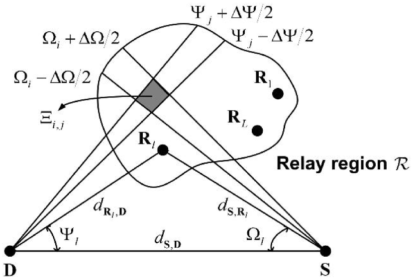
   Figure 1: Double-directional DWRN channel

3. Decode-and-forward Processing: Each $\mathbf{R}_{l}$ receives information from $\mathbf{S}$ in the first hop (backward channel) and then forwards the decoded signal to $\mathbf{D}$ in the second hop (forward channel). Two orthogonal frequency tones are used at these two transmission phases, respectively.

4. Medium Access: Due to the decentralized and unregulated nature of relay positions, a simplified time-division protocol is applied, which requires no knowledge of the network geometry at either $\mathbf{S}$ or $\mathbf{D}$. At the initial time $t=t_{0}$, $\mathbf{S}$ transmits its signal to all $\mathbf{R}_{l}$ $(l=1,2,\cdots,L)$. For the $l\mathrm{th}$ relay, it listens to the transmission from $\mathbf{S}$ in the time interval $\left[t_{0},t_{0}+{\Delta}t_{l}^{(\mathbf{B})}\right]$. After processing the received signals from $\mathbf{S}$, $\mathbf{R}_{l}$ forwards the message to $\mathbf{D}$ within $\left[t_{0}+{\Delta}t_{l}^{(\mathbf{B})},t_{0}+{\Delta}t_{l}^{(\mathbf{B})}+{\Delta}t_{l}^{(\mathbf{F})}\right]$. The two parameters ${\Delta}t_{l}^{(\mathbf{B})}$ and ${\Delta}t_{l}^{(\mathbf{F})}$ denote the time spent in the backward and forward phases, respectively. The same time-division process repeats in the subsequent time slots $\Big{[}t_{0}+k\times\left({\Delta}t_{l}^{(\mathbf{B})}+{\Delta}t_{l}^{(\mathbf{F})}\right),t_{0}+(k+1)\times\left({\Delta}t_{l}^{(\mathbf{B})}+{\Delta}t_{l}^{(\mathbf{F})}\right)\Big{]}$ $(k=1,2,\cdots)$. For simplicity, each relay spends equal times in its listening and forwarding phases. Apparently, $\mathbf{R}_{l}$ introduces an AOD $\Omega_{l}$ and an AOA $\Psi_{l}$ during each transmission cycle as shown in Fig. 1. It is worth emphasizing that the time-of-arrival (TOA) $\tau_{l}=\frac{d_{\mathbf{S},\mathbf{R}_{l}}+d_{\mathbf{R}_{l},\mathbf{D}}}{c}$, which is one of the key quantities used in the multipath channels [8], has lost its physical meaning in the current context. Here $d_{\mathbf{S},\mathbf{R}_{l}}$ and $d_{\mathbf{R}_{l},\mathbf{D}}$ are the distances of the links $\mathbf{S}\rightarrow\mathbf{R}_{l}$ and $\mathbf{R}_{l}\rightarrow\mathbf{D}$, respectively, and $c$ is the speed of electromagnetic waves.

5. Frequency-Tone Assignment: In general, mutual interference among the forward channels may incur due to the simultaneously transmitting relays. One way to eliminate the interference is to assign $L$ frequency tones drawn from the pool of available bandwidth $\left[\omega_{\mathrm{min}},\omega_{\mathrm{max}}\right]$ to $L$ relay-to-destination pairs, all of which are also orthogonal to the carrier allocated to the backward channels.

II-B Double-Directional Representation of DWRN

For a two-hop DWRN, multiple information pipelines are laid via the $L$ links $\mathbf{S}\rightarrow\mathbf{R}_{1}\rightarrow\mathbf{D},\cdots,\mathbf{S}\rightarrow\mathbf{R}_{L}\rightarrow\mathbf{D}$. Furthermore, the intersection of each AOD and each AOA uniquely determines the location of a relay. Therefore, as an ideal reference model, the information flows in the network are continuously distributed in the AOD-AOA domain as

$$I_{\mathrm{D}}(\Omega,\Psi)=\sum^{L}_{l=1}I_{l}\delta\left(\Omega-\Omega_{l}\right)\delta\left(\Psi-\Psi_{l}\right)$$ (1)

where $I_{\mathrm{D}}(\Omega,\Psi)$ is defined as the double-directional IAS and $I_{l}$ is the outage capacity given an outage probability of $P_{\mathrm{out}}$ for the link $\mathbf{S}\rightarrow\mathbf{R}_{l}\rightarrow\mathbf{D}$. The terminology double-directional is adopted according to [8].

Eq. (1) assumes perfect receivers that are able to resolve the departing and arriving information flows with infinite sensitivity in the angular domain. Therefore, the formulation represents an ideal benchmark model. In practice, both the source and destination have limited system sensitivity. Consider two data streams via two relays $\mathbf{R}_{l_{1}}$ and $\mathbf{R}_{l_{2}}$ $(1{\leq}l_{1}{\neq}l_{2}{\leq}L)$. Due to the finite length of the transmit (receive) antenna aperture, the AODs (AOAs) of these two information flows cannot be successfully distinguished if the separation of their departing (impinging) angles, $|\Omega_{l_{1}}-\Omega_{l_{2}}|$ $(|\Psi_{l_{1}}-\Psi_{l_{2}}|)$, is within the resolution limit of the source (destination) antenna, $\Delta\Omega$ $(\Delta\Psi)$. Therefore, the DWRN channel should be sampled at uniformly-spaced AODs and AOAs:

$$\begin{split}\Omega_{i}=i\Delta\Omega,~{}~{}~{}~{}~{}~{}~{}~{}~{}~{}\left\lfloor\frac{\Omega_{\mathrm{min}}}{\Delta\Omega}\right\rfloor{\leq}i{\leq}\left\lceil\frac{\Omega_{\mathrm{max}}}{\Delta\Omega}\right\rceil\\ \end{split}$$ (2)

$$\begin{split}\Psi_{j}=j\Delta\Psi,~{}~{}~{}~{}~{}~{}~{}~{}~{}~{}\left\lfloor\frac{\Psi_{\mathrm{min}}}{\Delta\Psi}\right\rfloor{\leq}j{\leq}\left\lceil\frac{\Psi_{\mathrm{max}}}{\Delta\Psi}\right\rceil\\ \end{split}$$ (3)

where ${\lfloor}\cdot\rfloor$ and ${\lceil}\cdot\rceil$ are the floor and ceiling functions, respectively.

Subsequently, the discrete double-directional IAS can be expressed as

$$\begin{split}I^{(\mathrm{d})}_{\mathrm{D}}\left(\Omega_{i},\Psi_{j}\right)&=\iint_{\Xi_{i,j}}I_{\mathrm{D}}(\Omega,\Psi)f^{(i,j)}_{\Omega,\Psi}(\Omega,\Psi)d{\Omega}d\Psi,\\ \mathrm{where}~{}\Xi_{i,j}&\triangleq\Bigg{\{}\left(\Omega,\Psi\right):\Omega_{i}-\frac{\Delta\Omega}{2}\leq\Omega\leq\Omega_{i}+\frac{\Delta\Omega}{2}\\ &~{}~{}~{}~{}~{}~{}~{}~{}~{}~{}~{}~{}~{}\&~{}\Psi_{j}-\frac{\Delta\Psi}{2}\leq\Psi\leq\Psi_{j}+\frac{\Delta\Psi}{2}\Bigg{\}}\end{split}$$ (4)

In (4), The superscript ^(d) denotes a discrete model. The local joint AOD-AOA pdf $f^{(i,j)}_{\Omega,\Psi}(\Omega,\Psi)$ satisfies $\iint_{\Xi_{i,j}}f^{(i,j)}_{\Omega,\Psi}(\Omega,\Psi)d{\Omega}d\Psi=1$, where the integration domain $\Xi_{i,j}$ is illustrated in Fig. 1.

III Geometrically-Based Statistical Model for a Random DWRN

We will discuss the proposed analytical framework in Section II from a geometrically-based statistical modeling perspective [6], where a large number of relays are randomly located in the two-dimensional space according to a specified relay density function. This approach is useful when the spatial structure observed in a large DWRN is far from being regular [11]. The medium access arrangement follows the protocol in Section II-A. Moreover, all channels experience independent frequency-flat block fading with the complex channel gain between the link $\mathbf{M}\rightarrow\mathbf{N}$, $h_{\mathbf{M},\mathbf{N}}$ $\left(\mathbf{M}\in\left\{\mathbf{S},\mathbf{R}_{1},\cdots,\mathbf{R}_{L}\right\},\mathbf{N}\in\left\{\mathbf{D},\mathbf{R}_{1},\cdots,\mathbf{R}_{L}\right\}\right)$ following the Nakagami distribution with shape parameter $m$ [8].

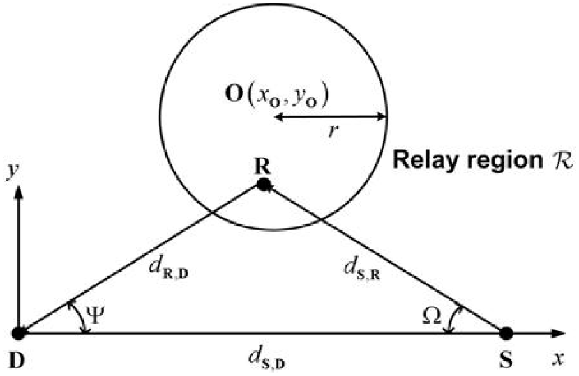
Figure 2: Geometrically-based statistical model for a DWRN

The associated instantaneous power $|h_{\mathbf{M},\mathbf{N}}|^{2}$ is gamma-distributed with the same shape parameter, i.e., $|h_{\mathbf{M},\mathbf{N}}|^{2}\sim\mathcal{G}\left(m,\frac{\lambda_{\mathbf{M},\mathbf{N}}}{m}\right)$, where $\mathcal{G}(\kappa,\theta)$ represents the gamma distribution with scale $\theta$ and shape $\kappa$. The mean value $\lambda_{\mathbf{M},\mathbf{N}}=d^{\nu}_{\mathbf{M},\mathbf{N}}$ with $\nu$ being the path loss exponent. The ambient noise at the relays and the destination, $Z_{\mathbf{N}}\sim\mathcal{N}(0,N_{0})$, where $\mathcal{N}(\mu,\sigma^{2})$ represents a normal distribution with mean $\mu$ and variance $\sigma^{2}$. The communication bandwidth is $B$ for any channel. Subsequently, the average received signal-to-noise ratio (SNR) for each link is $\mathrm{SNR}=\frac{P}{BN_{0}}$, where $P$ is the average transmit power for all transmitting terminals. Finally, the channel state information is assumed to be known at the receivers but unavailable to the transmitters [1].

Let the $x$-$y$ coordinate system be defined such that the destination is at the origin and the source lies on the $x$ axis, as shown in Fig. 2. It is assumed that there are many relay nodes, the locations of which are described by the statistical relay density function $f_{x,y}(x,y)$. By applying the law of sines to the triangle $\mathbf{SRD}$ in Fig. 2, the relay-to-destination distance $d_{\mathbf{R},\mathbf{D}}$ can be expressed in terms of the AOD $\Omega$ and the AOA $\Psi$ as

$$d_{\mathbf{R},\mathbf{D}}=\frac{d_{\mathbf{S},\mathbf{D}}\sin\Omega}{\sin(\Omega+\Psi)}$$ (5)

The source-to-relay distance $d_{\mathbf{S},\mathbf{R}}$ is similarly derived as

$$d_{\mathbf{S},\mathbf{R}}=\frac{d_{\mathbf{S},\mathbf{D}}\sin\Psi}{\sin(\Omega+\Psi)}$$ (6)

Proposition 1 (Derivation of $f_{\Omega,\Psi}(\Omega,\Psi)$):

The joint AOD-AOA pdf of information flows within a DWRN is given by

$$\begin{split}f_{\Omega,\Psi}(\Omega,\Psi)&=\frac{d^{2}_{\mathbf{S},\mathbf{D}}\left|\sin 2\Omega+\sin 2\Psi-\sin 2(\Omega+\Psi)\right|}{\left[1-\cos 2(\Omega+\Psi)\right]^{2}}\\ &{\times}f_{x,y}\left(\frac{d_{\mathbf{\mathbf{S},\mathbf{D}}}\sin\Omega\cos\Psi}{\sin(\Omega+\Psi)},\frac{d_{\mathbf{\mathbf{S},\mathbf{D}}}\sin\Omega\sin\Psi}{\sin(\Omega+\Psi)}\right)\end{split}$$ (7)

where $d_{\mathbf{S},\mathbf{D}}$ is the distance between the source and the destination.

Proof: The proof is omitted here for simplicity.

Proposition 2 (Derivation of $I_{\mathrm{D}}(\Omega,\Psi)$):

The double-directional IAS $I_{\mathrm{D}}(\Omega,\Psi)$ is the argument of the function

$$\begin{split}&\mathcal{P}\left(I\right)\\ &=1-\left[1-\frac{\gamma\left(m,\frac{m\left(4^{I}-1\right)}{\mathrm{SNR}{\times}d^{\nu}_{\mathbf{S},\mathbf{R}}}\right)}{\Gamma(m)}\right]\left[1-\frac{\gamma\left(m,\frac{m\left(4^{I}-1\right)}{\mathrm{SNR}{\times}d^{\nu}_{\mathbf{R},\mathbf{D}}}\right)}{\Gamma(m)}\right]\end{split}$$ (8)

when $\mathcal{P}\left(I\right)=P_{\mathrm{out}}$. In (8), $\gamma(\alpha,\beta)=\int^{\beta}_{0}t^{\alpha-1}e^{-t}dt$ is the lower incomplete gamma function and $\Gamma(\cdot)$ is the gamma function.

Proof: The proof is omitted here for simplicity.

Finally, the local joint AOD-AOA pdf in (4), $f^{(i,j)}_{\Omega,\Psi}(\Omega,\Psi)$, is related to $f_{\Omega,\Psi}(\Omega,\Psi)$ through the following relationship:

$$f^{(i,j)}_{\Omega,\Psi}(\Omega,\Psi)=\frac{f_{\Omega,\Psi}(\Omega,\Psi)}{\iint_{\Xi_{i,j}}f_{\Omega,\Psi}(\Omega,\Psi)d{\Omega}d\Psi}$$ (9)

Substituting (7)-(9) into (4) gives the discrete double-directional IAS.

IV RNT for a DWRN

IV-A Formulation of RNT

In the general RNT problem depicted in Fig. 3, $L$ relays $\left(\mathbf{R}_{1},\cdots,\mathbf{R}_{L}\right)$ are randomly scattered in a finite area $\mathcal{R}$ and $Q$ measuring nodes $\left(\mathbf{N}_{1},\cdots,\mathbf{N}_{Q}\right)$ are placed exterior to $\mathcal{R}$. Nevertheless, the following analysis is also applicable to any other measurement network orientation with respect to $\mathcal{R}$. Each measuring node can serve as the probing source as well as the information destination, which has a transmit/receive azimuthal resolution of $\Delta\Theta$. As shown in Fig. 3, the first node $\mathbf{N}_{1}$ transmits over its full spectrum of AODs $i\Delta\Theta~{}\left(i=\left\lfloor\frac{\Omega^{(1)}_{\min}}{\Delta\Theta}\right\rfloor,\left\lfloor\frac{\Omega^{(1)}_{\min}}{\Delta\Theta}\right\rfloor+1,\cdots,\left\lceil\frac{\Omega^{(1)}_{\max}}{\Delta\Theta}\right\rceil\right)$, where the superscript ⁽¹⁾ denotes $\mathbf{N}_{1}$. All other nodes $\mathbf{N}_{2}\sim\mathbf{N}_{Q}$ record an information flow. Each receive node $\mathbf{N}_{q}~{}(q=2,\cdots,Q)$ scans its entire angular range $j\Delta\Theta~{}\left(j=\left\lfloor\frac{\Psi^{(q)}_{\min}}{\Delta\Theta}\right\rfloor,\left\lfloor\frac{\Psi^{(q)}_{\min}}{\Delta\Theta}\right\rfloor+1,\cdots,\left\lceil\frac{\Psi^{(q)}_{\max}}{\Delta\Theta}\right\rceil\right)$, where the superscript ^(q) denotes $\mathbf{N}_{q}$. At each $j\Delta\Theta$, $\mathbf{N}_{q}$ searches the whole frequency band within which the relays are operating. When $\mathbf{N}_{q}$ locks on the $l{\mathrm{th}}$ frequency component $\omega_{l}$, which yields a detectable information flow associated with the relay $\mathbf{R}_{l}$, it then monitors the instantaneous channel capacity over an observation period and records the time-variant capacity $\hat{I}\left(t\right)$. From the set of $\hat{I}\left(t\right)$, the channel outage capacity $\hat{I}^{(1,q)}_{l}$ can be estimated empirically, where the superscript ^(1,q) denotes the information pathway from $\mathbf{N}_{1}$ to $\mathbf{N}_{q}$. The similar process continues until all the active relays are identified. Then the second node $\mathbf{N}_{2}$ sends the probing message and all the other nodes $\mathbf{N}_{1},\mathbf{N}_{3},\cdots,\mathbf{N}_{Q}$ receive the data, and so on.

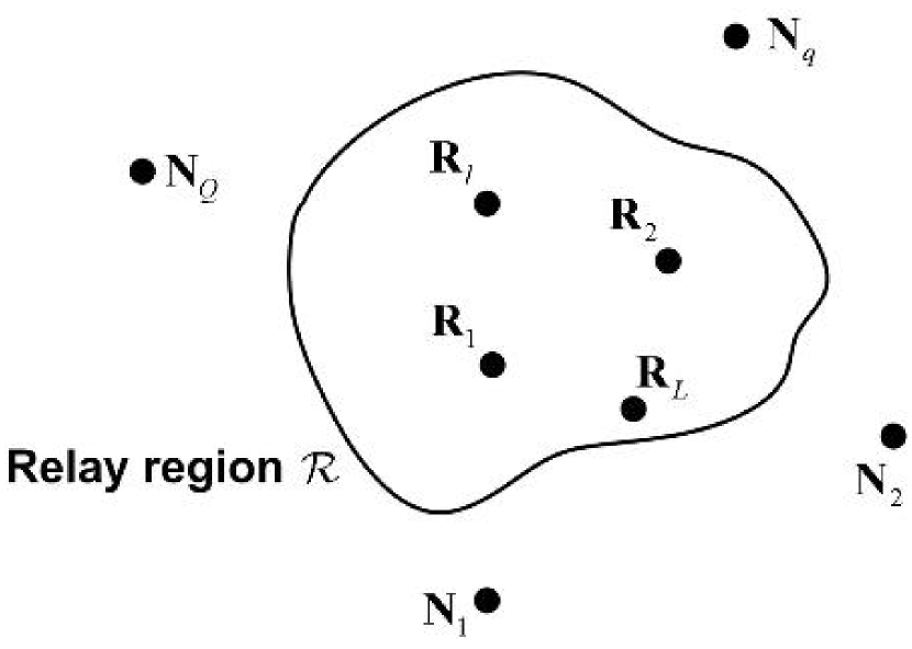
Figure 3: Formulation of RNT

A procedure to calculate the double-directional IAS for a DWRN with given sources, relays and destinations is called the direct problem. A procedure to obtain relay distribution knowing sources/destinations and measuring the information flows at multiple receivers is called the inverse problem. The direct problem has already been discussed in Section III. The corresponding inverse problem can be formulated as follows.

RNT Problem: Given the set of measuring nodes $\mathbf{N}_{1},\cdots,\mathbf{N}_{Q}$, the estimated $(Q-1)^{2}{\times}L$ single-directional AOA matrix

$$\begin{split}\mathbf{\bar{\hat{\Psi}}}&=\left[\begin{array}[]{cccc}\hat{\mathbf{\Psi}}_{1}&\hat{\mathbf{\Psi}}_{2}&\cdots&\hat{\mathbf{\Psi}}_{L}\\ \end{array}\right]\\ &=\left[\begin{array}[]{ccccc}\hat{\Psi}^{(1,2)}_{1}&\hat{\Psi}^{(1,2)}_{2}&\cdots&\hat{\Psi}^{(1,2)}_{L}\\ \vdots&\vdots&\ddots&\vdots\\ \hat{\Psi}^{(Q,Q-1)}_{1}&\hat{\Psi}^{(Q,Q-1)}_{2}&\cdots&\hat{\Psi}^{(Q,Q-1)}_{L}\\ \end{array}\right]\end{split}$$ (10)

and the estimated $(Q-1)^{2}{\times}L$ outage capacity matrix

$$\begin{split}\mathbf{\bar{\hat{I}}}&=\left[\begin{array}[]{cccc}\hat{\mathbf{I}}_{1}&\hat{\mathbf{I}}_{2}&\cdots&\hat{\mathbf{I}}_{L}\\ \end{array}\right]\\ &=\left[\begin{array}[]{ccccc}\hat{I}^{(1,2)}_{1}&\hat{I}^{(1,2)}_{2}&\cdots&\hat{I}^{(1,2)}_{L}\\ \vdots&\vdots&\ddots&\vdots\\ \hat{I}^{(Q,Q-1)}_{1}&\hat{I}^{(Q,Q-1)}_{2}&\cdots&\hat{I}^{(Q,Q-1)}_{L}\\ \end{array}\right]\end{split}$$ (11)

$\hat{\Psi}^{\left(q_{1},q_{2}\right)}_{l}$ and $\hat{I}^{\left(q_{1},q_{2}\right)}_{l}$ are the empirical AOA and channel outage capacity associated with the information pipeline $\mathbf{N}_{q_{1}}\rightarrow\mathbf{R}_{l}\rightarrow\mathbf{N}_{q_{2}}$, respectively. Note that due to the channel reciprocity in a two-hop DWRN, it is expected that $\hat{\Psi}^{\left(q_{1},q_{2}\right)}_{l}=\hat{\Omega}^{\left(q_{2},q_{1}\right)}_{l}$ and $\hat{I}^{\left(q_{1},q_{2}\right)}_{l}=\hat{I}^{\left(q_{2},q_{1}\right)}_{l}$. Therefore, (11) is equivalent to a double-directional AOD-AOA matrix, where half of the AOAs correspond to the AODs of the reversed information pathways. Identify the locations of $\mathbf{R}_{1},\cdots,\mathbf{R}_{L}$ that satisfy the following two constraint functions

$$e_{1}\left(\mathbf{\hat{\Psi}}_{l}-\mathbf{\Psi}_{l}\right)\leq\epsilon_{1},~{}~{}~{}~{}~{}~{}~{}~{}l=1,2,\cdots,L$$ (12)

and

$$e_{2}\left(\mathbf{\hat{I}}_{l}-\mathbf{I}_{l}\right)\leq\epsilon_{2},~{}~{}~{}~{}~{}~{}~{}~{}l=1,2,\cdots,L$$ (13)

$\mathbf{\Psi}_{l}$ and $\mathbf{I}_{l}$ are the AOA and channel outage capacity vectors solved in the direct problem for all the information paths via $\mathbf{R}_{l}$ assuming a specific location of $\mathbf{R}_{l}$.

IV-B Algorithms to Solve The RNT Problem

In the current work, we will consider the $\ell^{2}$-norm of the two error vectors, i.e., $e_{1}\left(\mathbf{\hat{\Psi}}_{l}-\mathbf{\Psi}_{l}\right)=\sqrt{\sum_{q_{1}}\sum_{q_{2}{\neq}q_{1}}\left(\hat{\Psi}^{\left(q_{1},q_{2}\right)}_{l}-\Psi^{\left(q_{1},q_{2}\right)}_{l}\right)^{2}}$ and $e_{2}\left(\mathbf{\hat{I}}_{l}-\mathbf{I}_{l}\right)=\sqrt{\sum_{q_{1}}\sum_{q_{2}{\neq}q_{1}}\left(\hat{I}^{\left(q_{1},q_{2}\right)}_{l}-I^{\left(q_{1},q_{2}\right)}_{l}\right)^{2}}$. The objectives are to minimize the values of $e_{2}$ and meanwhile ensure that $e_{1}=0$ for all the detectable information flows. The optimization process can be realized through the following steps:

$1)$ Discretize the solution domain of the relay locations $\mathcal{R}$ into $W$ sufficiently small square cells, i.e., $\mathbb{R}=\mathcal{R}^{(\mathrm{d})}\triangleq\left\{\mathbf{x}_{1},\cdots,\mathbf{x}_{W}\right\}$, where $\mathbf{x}_{w}=(x_{w},y_{w})~{}(w=1,2,\cdots,W)$ represents the Cartesian coordinates of the center of the $w{\mathrm{th}}$ cell;

$2)$ For each identified information pipeline $\mathbf{N}_{q_{1}}\rightarrow\mathbf{R}_{l}\rightarrow\mathbf{N}_{q_{2}}$, determine the subset of $\mathbb{R}$, $\mathbb{R}^{\left(q_{1},q_{2}\right)}_{l}\subseteq\mathbb{R}$, such that ${\forall}\mathbf{x}\in\mathbb{R}^{\left(q_{1},q_{2}\right)}_{l}$, $\hat{\Psi}^{\left(q_{1},q_{2}\right)}_{l}=\Psi^{\left(q_{1},q_{2}\right)}_{l}(\mathbf{x})$;

$3)$ Determine the joint of all the sets obtained in Step 2 as $\mathbb{R}_{l}=\mathbb{R}^{(1,2)}_{l}\bigcap\mathbb{R}^{(1,3)}_{l}\bigcap\cdots\bigcap\mathbb{R}^{(Q,Q-1)}_{l}$;

$4)$ Estimate the location of $\mathbf{R}_{l}$ as

$$\mathbf{x}\left(\mathbf{R}_{l}\right)=\mathrm{arg}\min_{\mathbf{x}\in\mathbb{R}_{l}}\sqrt{\sum_{q_{1}}\sum_{q_{2}{\neq}q_{1}}\left(\hat{I}^{\left(q_{1},q_{2}\right)}_{l}-I^{\left(q_{1},q_{2}\right)}_{l}(\mathbf{x})\right)^{2}}$$ (14)

It is not always possible to obtain an accurate estimate of the outage capacity $\hat{I}^{\left(q_{1},q_{2}\right)}_{l}$ due to the limited observation data at each destination. In such a case, the inverse problem could be approached from a hypothesis-testing perspective. An alternative optimization procedure to Step 4 can be formulated as follows.

$4^{\star})$ Let there be $K$ relay-position hypotheses denoted $\mathcal{H}_{1}:\mathbf{x}(\mathbf{R}_{l})=\mathbf{\tilde{x}}_{1}$,$\mathcal{H}_{2}:\mathbf{x}(\mathbf{R}_{l})=\mathbf{\tilde{x}}_{2}$, $\cdots$,$\mathcal{H}_{K}:\mathbf{x}(\mathbf{R}_{l})=\mathbf{\tilde{x}}_{K}$, where $K=|\mathbb{R}_{l}|$ and $\mathbb{R}_{l}=\left\{\mathbf{\tilde{x}}_{1},\mathbf{\tilde{x}}_{2},\cdots,\mathbf{\tilde{x}}_{K}\right\}$. Furthermore, let $\varepsilon_{k_{1},k_{2}}$ be the desired probability of incorrectly selecting $\mathcal{H}_{k_{2}}$ given that $\mathcal{H}_{k_{1}}$ is true. The sequential probability ratio test procedures will be applied for statistical decision making, where the decision at each stage is based on the likelihood ratio. In particular, the multi-hypothesis sequential test is considered and summarized below [12]. The likelihood ratio including prior probabilities for a pair of hypotheses $k_{1}$ and $k_{2}$ after the $o{\mathrm{th}}$ data observation is

$$\eta^{o}_{k_{1},k_{2}}=\frac{f_{\mathcal{H}_{k_{1}}}(\mathfrak{I}_{1})f_{\mathcal{H}_{k_{1}}}(\mathfrak{I}_{2}){\cdots}f_{\mathcal{H}_{k_{1}}}(\mathfrak{I}_{o})\mathrm{Pr}\left(\mathcal{H}_{k_{1}}\right)}{f_{\mathcal{H}_{k_{2}}}(\mathfrak{I}_{1})f_{\mathcal{H}_{k_{2}}}(\mathfrak{I}_{2}){\cdots}f_{\mathcal{H}_{k_{2}}}(\mathfrak{I}_{o})\mathrm{Pr}\left(\mathcal{H}_{k_{2}}\right)}$$ (15)

where $\mathfrak{I}_{o}=\left(\mathcal{I}^{(1,2)}_{l,o},\mathcal{I}^{(1,3)}_{l,o},\cdots,\mathcal{I}^{(Q,Q-1)}_{l,o}\right)^{T}$ is the instantaneous outage capacity vector at the $o{\mathrm{th}}$ observation for all the information routes via $\mathbf{R}_{l}$. $f_{\mathcal{H}_{k_{1}}}(\mathfrak{I}_{o})$ is the pdf of $\mathfrak{I}_{o}$ under $\mathcal{H}_{k_{1}}$, which is given by

$$\begin{split}&f_{\mathcal{H}_{k_{1}}}(\mathfrak{I}_{o})\stackrel{{\scriptstyle(a)}}{{=}}\prod_{q_{1}}\prod_{q_{2}{\neq}q_{1}}f_{\mathcal{I}}\left(\mathcal{I}^{(q_{1},q_{2})}_{l,o};\mathbf{x}(\mathbf{R}_{l})=\mathbf{\tilde{x}}_{k_{1}}\right)\\ &\stackrel{{\scriptstyle(b)}}{{=}}\ln 4\times\prod_{q_{1}}\prod_{q_{2}{\neq}q_{1}}\Bigg{\{}\left[\rho_{1}\left(\mathcal{I}^{(q_{1},q_{2})}_{l,o},\mathbf{\tilde{x}}_{k_{1}}\right)\right]^{m}\\ &~{}~{}~{}~{}~{}~{}~{}~{}~{}~{}~{}~{}~{}~{}~{}~{}~{}~{}~{}~{}~{}~{}~{}~{}~{}~{}\times\exp\left[{-\rho_{1}\left(\mathcal{I}^{(q_{1},q_{2})}_{l,o},\mathbf{\tilde{x}}_{k_{1}}\right)}\right]\\ &~{}~{}~{}~{}~{}~{}~{}~{}~{}~{}~{}~{}~{}~{}~{}~{}~{}~{}~{}~{}~{}~{}~{}~{}~{}~{}\times\left[1-\frac{\gamma\left(m,\rho_{2}\left(\mathcal{I}^{(q_{1},q_{2})}_{l,o},\mathbf{\tilde{x}}_{k_{1}}\right)\right)}{\Gamma(m)}\right]\\ &~{}~{}~{}~{}~{}~{}~{}~{}~{}~{}~{}~{}~{}~{}~{}~{}~{}~{}~{}~{}~{}~{}+\left[\rho_{2}\left(\mathcal{I}^{(q_{1},q_{2})}_{l,o}\right),\mathbf{\tilde{x}}_{k_{1}}\right]^{m}\\ &~{}~{}~{}~{}~{}~{}~{}~{}~{}~{}~{}~{}~{}~{}~{}~{}~{}~{}~{}~{}~{}~{}~{}~{}~{}~{}\times\exp\left[{-\rho_{2}\left(\mathcal{I}^{(q_{1},q_{2})}_{l,o},\mathbf{\tilde{x}}_{k_{1}}\right)}\right]\\ &~{}~{}~{}~{}~{}~{}~{}~{}~{}~{}~{}~{}~{}~{}~{}~{}~{}~{}~{}~{}~{}~{}~{}~{}~{}~{}\times\left[1-\frac{\gamma\left(m,\rho_{1}\left(\mathcal{I}^{(q_{1},q_{2})}_{l,o},\mathbf{\tilde{x}}_{k_{1}}\right)\right)}{\Gamma(m)}\right]\Bigg{\}}\end{split}$$ (16)

where $(a)$ follows the fact that the instantaneous outage capacities are sequentially observed for all the information paths via $\mathbf{R}_{l}$ during the measurement process. Therefore, they can be assumed to be independently distributed. The equality in $(b)$ is obtained by differentiating the cdf in (8) with respect to the variable $I$. In (16),

$$\rho_{1}\left(\mathcal{I}^{(q_{1},q_{2})}_{l,o},\mathbf{\tilde{x}}_{k_{1}}\right)=\frac{m\left(4^{\mathcal{I}^{(q_{1},q_{2})}_{l,o}}-1\right)}{\mathrm{SNR}{\times}\left[d_{\mathbf{S},\mathbf{R}}\left(\mathbf{\tilde{x}}_{k_{1}}\right)\right]^{\nu}}$$

and

$$\rho_{2}\left(\mathcal{I}^{(q_{1},q_{2})}_{l,o},\mathbf{\tilde{x}}_{k_{1}}\right)=\frac{m\left(4^{\mathcal{I}^{(q_{1},q_{2})}_{l,o}}-1\right)}{\mathrm{SNR}{\times}\left[d_{\mathbf{R},\mathbf{D}}\left(\mathbf{\tilde{x}}_{k_{1}}\right)\right]^{\nu}}$$

If the number of observations is not fixed, a decision on the relay-position state (i.e., $\mathcal{H}_{\hat{k}}$ is selected) is made when the condition

$$\eta^{o}_{\hat{k},k_{2}}>\frac{1-\varepsilon_{\hat{k},k_{2}}}{\varepsilon_{\hat{k},k_{2}}}~{}~{}~{}\forall\hat{k}{\neq}k_{2}$$ (17)

is met. The threshold in (17) to which the likelihood ratio is compared is designed to ensure that the average rate of making a wrong decision in favor of $\mathcal{H}_{k_{2}}$ when $\mathcal{H}_{k_{1}}$ is true is no more than $\varepsilon_{k_{1},k_{2}}$. Nevertheless, the inequality in (17) may not always be satisfied due to the insufficient observation data. In such a case, a hypotheses $\mathcal{H}_{\hat{k}}$ is selected if its associated likelihood has the maximum value after a fixed number of $O$ observations, i.e.,

$$\hat{k}=\mathrm{arg}\max_{k}~{}f_{\mathcal{H}_{k}}(\mathfrak{I}_{1})f_{\mathcal{H}_{k}}(\mathfrak{I}_{2}){\cdots}f_{\mathcal{H}_{k}}(\mathfrak{I}_{O})\mathrm{Pr}\left(\mathcal{H}_{k}\right)$$ (18)

Eqs. (17) and (18) provide alternative objective functions to the one given in (14).

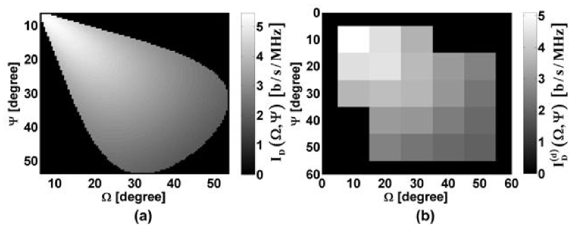
Figure 4: Double-directional IAS: (a) continuous reference model and (b) discrete model for systems with an angular resolution of $10^{\circ}$

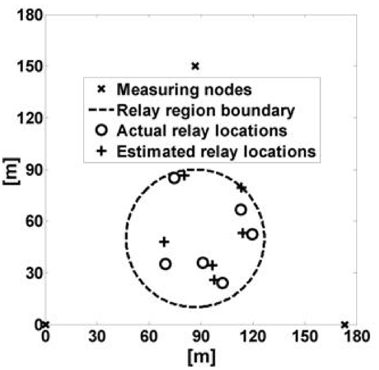
Figure 5: Estimation of relay locations using the proposed RNT algorithm

V Numerical Examples

We consider the high SNR regime ($\mathrm{SNR}=30~{}\mathrm{dB}$) for a fixed outage probability $P_{\mathrm{out}}=0.01$. The shape parameter of the Nakagami distribution is $m=1$ (Rayleigh fading). The distance between the source and the destination $d_{\mathbf{S},\mathbf{D}}$ is assumed to be $100\sqrt{3}~{}\mathrm{m}$ (see also Fig. 2) and the path loss exponent is $\nu=-3$. The relay region is assumed to be a circle centered at $\mathbf{O}(50\sqrt{3}~{}\mathrm{m},50~{}\mathrm{m})$ with a radius $r=40~{}\mathrm{m}$. Finally, the spatial resolutions of both the source and destination antennas are $10^{\circ}$.

Fig. 4 illustrates the double-directional IAS for both the continuous reference model in (1) and its discrete counterpart in (4). Apparently, both $I_{\mathrm{D}}(\Omega,\Psi)$ and $I^{(\mathrm{d})}_{\mathrm{D}}(\Omega,\Psi)$ decrease as the AOD $\Omega$ and the AOA $\Psi$ increase. This certainly holds an intuitive appeal because larger values of $\Omega$ and $\Psi$ lead to more severe path loss, thereby reducing the outage capacity of a relay path. As a practical concern, Fig. 4 provides an intuitive and quantitative answer to the following two important questions: how will the information flows be scattered in the AOD and AOA domains and what will be the beam-scanning ranges of the source and destination antennas in order to achieve sufficiently high outage capacities?

Next, we look into the RNT problem discussed in Section IV. A three-node measurement network is deployed as illustrated in Fig. 5. A number of relays are uniformly distributed within a circular region. The procedures presented in Section IV-B are applied to estimate the relay locations, where the objective function of (18) is used. The number of observations of the instantaneous channel capacity for each information pipeline is $O=10$. Furthermore, no a priori knowledge of the probability of each location under hypothesis test is available. As can be observed from Fig. 5, most of the estimated relay locations agree well with the actual ones, which demonstrates the efficacy of the proposed RNT algorithm by using a relatively small number of measuring nodes and observations.

VI Conclusions

We have presented a double-directional description method for analyzing two-hop DWRN channels, which is based on an analogous approach to the double-directional physical wireless channels. The proposed model has been investigated using a geometrically-based statistical modeling approach with uniformly distributed relay nodes. We have also investigated the RNT problem by applying the proposed network representation. Finally, numerical examples have been used to demonstrate the practical significance of the proposed analytical framework.

References

- [1] J. N. Laneman, D. N. C. Tse, and G. W. Wornell, “Cooperative diversity in wireless networks: Efficient protocols and outage behavior,” IEEE Trans. Inform. Theory, vol. 50, no. 12, pp. 3062–3080, 2004.
- [2] B. Wang, J. Zhang, and L. Zheng, “Achievable rates and scaling laws of power-constrained wireless sensory relay networks,” IEEE Trans. Inform. Theory, vol. 52, no. 9, pp. 4084–4104, 2006.
- [3] B. Sirkeci-Mergen and A. Scaglione, “On the power efficiency of cooperative broadcast in dense wireless networks,” IEEE J. Select. Areas Commun., vol. 25, no. 2, pp. 497–507, 2007.
- [4] A. Özgür, O. Lévêque, and D. N. C. Tse, “Hierarchical cooperation achieves optimal capacity scaling in ad hoc networks,” IEEE Trans. Inform. Theory, vol. 53, pp. 3549–3572, Oct. 2007.
- [5] S. Cui, A. M. Haimovich, O. Somekh, and H. V. Poor, “Decentralized two-hop opportunistic relaying with limited channel state information,” in Proc. IEEE International Symposium on Information Theory, Toronto, July 2008.
- [6] Y. Chen and P. Rapajic, “Decentralized wireless relay network channel modeling: An analogous approach to mobile radio channel characterization,” IEEE Trans. Commun., vol. 58, pp. 467–473, Feb. 2010.
- [7] K. I. Pedersen, P. E. Mogensen, and B. H. Fleury, “A stochastic model of the temporal and azimuthal dispersion seen at the base station in outdoor propagation environments,” IEEE Trans. Veh. Technol., vol. 49, no. 2, pp. 437–447, 2000.
- [8] A. F. Molisch, Wireless Communications, John Wiley and Sons, Chichester, West Sussex, 2005.
- [9] R. B. Ertel and J. H. Reed, “Angle and time of arrival statistics for circular and elliptical scattering models,” IEEE J. Sel. Areas Commun., vol. 17, no. 11, pp. 1829–1840, 1999.
- [10] A. C. Kak and M. Slaney, Principles of Computerized Tomographic Imaging, Society of Industrial and Applied Mathematics, 2001.
- [11] J. G. Andrews, N. Jindal, M. Haenggi, R. Berry, S. Jafar, D. Guo, S. Shakkottai, R. Heath, M. Neely, S. Weber, and A. Yener, “Rethinking information theory for mobile ad hoc networks,” IEEE Commun. Mag., vol. 46, pp. 94–101, Dec. 2008.
- [12] N. A. Goodman, P. R. Venkata, and M. A. Neifeld, “Adaptive waveform design and sequential hypothesis testing for target recognition with active sensors,” IEEE Journal of Selected Topics in Signal Processing, vol. 1, no. 1, pp. 105–113, 2007.