The Graph Traversal Pattern

Abstract

A graph is a structure composed of a set of vertices (i.e. nodes, dots) connected to one another by a set of edges (i.e. links, lines). The concept of a graph has been around since the late 19${}^{\text{th}}$ century, however, only in recent decades has there been a strong resurgence in both theoretical and applied graph research in mathematics, physics, and computer science. In applied computing, since the late 1960s, the interlinked table structure of the relational database has been the predominant information storage and retrieval model. With the growth of graph/network-based data and the need to efficiently process such data, new data management systems have been developed. In contrast to the index-intensive, set-theoretic operations of relational databases, graph databases make use of index-free, local traversals. This article discusses the graph traversal pattern and its use in computing.

1 Introduction

The first paragraph of any publication on graphs usually contains the iconic $G=(V,E)$ definition of a graph. This definition states that a graph is composed of a set of vertices $V$ and a set of edges $E$. Normally following this definition is the definition of the set $E$. For directed graphs, $E\subseteq(V\times V)$ and for undirected graphs, $E\subseteq\{V\times V\}$. That is, $E$ is a subset of all ordered or unordered permutations of $V$ element pairings. From a purely theoretical standpoint, such definitions are usually sufficient for deriving theorems. However, in applied research, where the graph is required to be embedded in reality, this definition says little about a graph’s realization. The structure a graph takes in the real-world determines the efficiency of the operations that are applied to it. It is exactly those efficient graph operations that yield an unconventional problem-solving style. This style of interaction is dubbed the graph traversal pattern and forms the primary point of discussion for this article.

2 The Realization of Graphs

Relational databases have been around since the late 1960s rdbms:codd1970 and are todays most predominate data management tool. Relational databases maintain a collection of tables. Each table can be defined by a set of rows and a set of columns. Semantically, rows denote objects and columns denote properties/attributes. Thus, the datum at a particular row/column-entry is the value of the column property for that row object. Usually, a problem domain is modeled over multiple tables in order to avoid data duplication. This process is known as data normalization. In order to unify data in disparate tables, a “join” is used. A join combines two tables when columns of one table refer to columns of another table. Maintaining these references in a consistent state is known as a referential integrity. This is the classic relational database design which affords them their flexibility join:mishra1992 .

In stark contrast, graph databases do not store data in disparate tables. Instead there is a single data structure—the graph. Moreover, there is no concept of a “join” operation as every vertex and edge has a direct reference to its adjacent vertex or edge. The data structure is already “joined” by the edges that are defined. There are benefits and drawbacks to this model. First, the primary drawback is that its difficult to shard a graph (a difficulty also encountered with relational databases that maintain referential integrity). Sharding is the process of partitioning data across multiple machines in order to scale a system horizontally. In a graph, with unconstrained, direct references between vertices and edges, there usually does not exist a clean data partition. Thus, it becomes difficult to scale graph databases beyond the confines of a single machine and at the same time, maintain the speed of a traversal across sharded borders. However, at the expense of this drawback there is a significant advantage: there is a constant time cost for retrieving an adjacent vertex or edge. That is, regardless of the size of the graph as a whole, the cost of a local read operation at a vertex or edge remains constant. This benefit is so important that it creates the primary means by which users interact with graph databases—traversals. Graphs offer a unique vantage point on data, where the solution to a problem is seen as abstractly defined traversals through its vertices and edges.

2.1 The Indices of Relational Tables

Imagine that there is a gremlin who is holding a number between 1 and 100 in memory. Moreover, assume that when guessing the number, the gremlin will only reply by saying whether the guessed number is greater than, less than, or equal to the number in memory. What is the best strategy for determining the number in the fewest guesses? On average, the quickest way to determine the number is to partition the space of guesses into equal size chunks. For example, ask if the number is 50. If the gremlin states that its less than 50, then ask, is the number 25? If greater than 25, then ask, is the number 37? Follow this partition scheme until the number is converged upon. The structure that these guesses form over the sequence from 1 to 100 is a binary search tree. On average, this tree structure is more efficient in time than guessing each number starting from 1 and going to 100. This is ultimately the difference between an index-based search and a linear search. If there were no indices for a set, every element of the set would have to be examined to determine if it has a particular property of interest. For $n$ elements, a linear scan of this nature runs in $\mathcal{O}(n)$. When elements are indexed, there exists two structures—the original set of elements and an index of those elements. Typical indices have the convenient property that searching them takes $\mathcal{O}(\text{log}_{2}n)$. For massive sets, the space that indices take is well worth their weight in time.

Relational databases take significant advantage of such indices. It is through indices that rows with a column value are efficiently found. Moreover, the index makes it possible to efficiently join tables together in order to move between tables that are linked by particular columns. Assume a simple example where there are two tables: a person table and a friend table. The person table has the following two columns: unique identifier and name. The friend table has the following two columns: person_a and person_b. The semantics of the friend table is that person $a$ is friends with person $b$. Suppose the problem of determining the name of all of Alberto Pepe’s friends. Figure 1 and the following list breaks down this simple query into all the micro-operations that must occur to yield results.

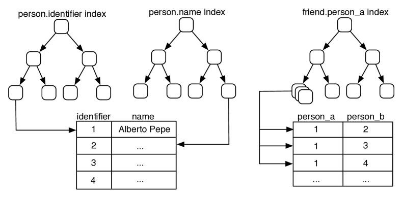
Figure 1: A table representation of people and their friends.

1. Query the person.name index to find the row in person with the name “Alberto Pepe.” [$\mathcal{O}(\text{log}_{2}n)$]

2. Given the person row returned by the index, get the identifier for that row.[$\mathcal{O}(1)$]

3. Query the friend.person_a index to find all the rows in friend with the identifier from previous. [$\mathcal{O}(\text{log}_{2}x):x\ll m$]

4. Given each of the $k$ rows returned, get the person_b identifier for those rows. [$\mathcal{O}(k)$]

5. For each $k$ friend identifiers, query the person.identifier index for the row with friend identifier. [$\mathcal{O}(k\;\text{log}_{2}n)$]

6. Given the $k$ person rows, get the name value for those rows. [$\mathcal{O}(k)$]

The final operation yields the names of Alberto’s friends. This example elucidates the classic join operation utilized in relational databases. By being able to join the person and friend table, its possible to move from a name, to the person, to his or her friends, and then, ultimately, to their names. In effect, the join operation forms a graph that is dynamically constructed as one table is linked to another table. While having the benefit of being able to dynamically construct graphs, the limitation is that this graph is not explicit in the relational structure, but instead must be inferred through a series of index-intensive operations. Moreover, while only a particular subset of the data in the database may be desired (e.g. only Alberto’s friend’s), all data in all queried tables must be examined in order to extract the desired subset (e.g. all friends of all people). Even though a $\mathcal{O}(\text{log}_{2}n)$ read-time is fast for a search, as the the indices grow larger with the growth of the data and as more join operations are used, this model becomes inefficient. At the limit, the inferred graph that is constructed through joins is best solved (with respects to time), by a graph database.

2.2 The Graph as an Index

Most of graph theory is concerned with the development of theorems for single-relational graphs graphs:chartrand1986 . A single-relational graph maintains a set of edges, where all the edges are homogeneous in meaning. For example, all edges denote friendship or kinship, but not both together within the same structure. In application, complex domain models are more conveniently represented by multi-relational, property graphs. The edges in a property graph are typed or labeled and thus, edges are heterogenous in meaning. For example, a property graph can model friendship, kinship, business, communication, etc. relationships all within the same structure. Moreover, vertices and edges in a property graph maintain a set of key/value pairs. These are known as properties and allow for the representation of non-graphical data—e.g. the name of a vertex, the weight of an edge, etc. Formally, a property graph can be defined as $G=(V,E,\lambda,\mu)$, where edges are directed (i.e. $E\subseteq(V\times V)$), edges are labeled (i.e. $\lambda:E\rightarrow\Sigma$), and properties are a map from elements and keys to values (i.e. $\mu:(V\cup E)\times R\rightarrow S$).

In the property graph model, it is common for the properties of the vertices (and sometimes edges) to be indexed using a tree structure analogous, in many ways, to those used by relational databases. This index can be represented by some external indexing system or endogenous to the graph as an embedded tree (see §3.2). Given the prior situation, once a set of elements have been identified by the index search, then a traversal is executed through the graph. Elements in a graph are adjacent to one another by direct references. A vertex is adjacent to its incoming and outgoing edges and an edge is adjacent to its outgoing (i.e. tail) and incoming (i.e. head) vertices. The domain model defines how the elements of the problem space are related. Similar to the gremlin stating that 50 is greater than the number to be guessed, an edge connecting vertex $i$ and $j$ and labeled friend states that vertex $i$ is friend related to vertex $j$. Indices create “short cuts” in the graph as they partition elements according to specialized, compute-centric semantics (e.g. numbers being less than or greater than another). Likewise, a domain model partitions elements using semantics defined by the domain modeler. Thus, in many ways, a graph can be seen as an indexing structure.

In the relational example previous, a person in the person table has two properties: a unique identifier and a name. The analogue in a property graph would be to have the identifier and name values represented as vertex properties. Moreover, the friend table would not exist as a table, but as direct friend-labeled edges between vertices. This idea is diagrammed in Figure 2. The micro-operations used to find the name of all of Alberto Pepe’s friends are provided in the following enumeration.

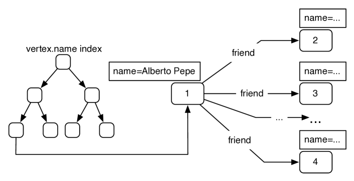
Figure 2: A graph representation of people and their friends. Given the tree-nature of the vertex.name index, it is possible, and many times useful to model the index endogenous to the graph (see §3.2).

1. Query the vertex.name index to find all the vertices in $G$ with the name “Alberto Pepe.” [$\mathcal{O}(\text{log}_{2}n)$]

2. Given the vertex returned, get the $k$ friend edges emanating from this vertex. [$\mathcal{O}(k+x)$]

3. Given the $k$ friend edges retrieved, get the $k$ vertices on the heads of those edges. [$\mathcal{O}(k)$]

4. Given these $k$ vertices, get the $k$ name properties of these vertices. [$\mathcal{O}(ky)$]

The final operation yields the names of Alberto’s friends. In a graph database, there is no explicit join operation because vertices maintain direct references to their adjacent edges. In many ways, the edges of the graph serve as explicit, “hard-wired” join structures (i.e. structures that are not computed at query time as in a relational database). The act of traversing over an edge is the act of joining. However, what makes this more efficient in a graph database is that traversing from one vertex to another is a constant time operation. Thus, traversal time is defined solely by the number of elements touched by the traversal. This is irrespective of the size/topology of the graph as a whole. The time it takes to make a single step in a traversal is determined by the local topology of the subgraph surrounding the particular vertex being traversed from.

The real power of graph databases makes itself apparent when traversing multiple steps in order to unite disparate vertices by a path (i.e. vertices not directly connected). First, there are no $\mathcal{O}(\text{log}_{2}n)$ operations. Second, the type of path taken, defines the “higher order,” inferred relationship that exists between two vertices. Traversals based on abstractly defined paths is the core of the graph traversal pattern. The next section discusses the graph traversal pattern and its application to common problem-solving situations.

3 Graph Traversals

A traversal refers to visiting elements (i.e. vertices and edges) in a graph in some algorithmic fashion. This section will present a functional, flow-based approach flow:morrison1994 to traversing property graphs and how different types of traversals over different types of graph datasets support different types of problem-solving.

The most primitive, read-based operation on a graph is a single step traversal from element $i$ to element $j$, where $i,j\in(V\cup E)$. For example, a single step operation can answer questions such as “which edges are outgoing from this vertex?”, “which vertex is at the head of this edge?”, etc. Single step operations expose explicit adjacencies in the graph (i.e. adjacencies that are “hard-wired”). The following list itemizes the various types of single step traversals. Note that these operations are defined over power multiset domains and ranges. The reason for this is that is naturally allows for function composition, where a composition is a formal description of a traversal.

• $e_{\text{out}}:\mathcal{\hat{P}}(V)\rightarrow\mathcal{\hat{P}}(E)$: traverse to the outgoing edges of the vertices.

• $e_{\text{in}}:\mathcal{\hat{P}}(V)\rightarrow\mathcal{\hat{P}}(E)$: traverse to the incoming edges to the vertices.

• $v_{\text{out}}:\mathcal{\hat{P}}(E)\rightarrow\mathcal{\hat{P}}(V)$: traverse to the outgoing (i.e. tail) vertices of the edges.

• $v_{\text{in}}:\mathcal{\hat{P}}(E)\rightarrow\mathcal{\hat{P}}(V)$: traverse the incoming (i.e. head) vertices of the edges.

• $\epsilon:\mathcal{\hat{P}}(V\cup E)\times R\rightarrow\mathcal{\hat{P}}(S)$: get the element property values for key $r\in R$.

When edges are labeled and elements have properties, it is desirable to constrain the traversal to edges of a particular label or elements with particular properties. These operations are known as filters and are abstractly defined in the following itemization.

• $e_{\text{lab}\pm}:\mathcal{\hat{P}}(E)\times\Sigma\rightarrow\mathcal{\hat{P}}(E)$: allow (or filter) all edges with the label $\sigma\in\Sigma$.

• $\epsilon_{\text{p}\pm}:\mathcal{\hat{P}}(V\cup E)\times R\times S\rightarrow\mathcal{\hat{P}}(V\cup E)$: allow (or filter) all elements with the property $s\in S$ for key $r\in R$.

• $\epsilon_{\epsilon\pm}:\mathcal{\hat{P}}(V\cup E)\times(V\cup E)\rightarrow\mathcal{\hat{P}}(V\cup E)$: allow (or filter) all elements that are the provided element.

Through function composition, we can define graph traversals of arbitrary length. A simple example is traversing to the names of Alberto Pepe’s friends. If $i$ is the vertex representing Alberto Pepe and

$$f:\mathcal{\hat{P}}(V)\rightarrow\mathcal{\hat{P}}(S),$$

where

$$f(i)=\epsilon\left(v_{\text{in}}\left(e_{\text{lab+}}\left(e_{\text{out}}(i),\text{friend}\right)\right),\text{name}\right),$$

then $f(i)$ will return the names of Alberto Pepe’s friends. Through function currying and composition, the previous definition can be represented more clearly with the following function rule,

$$f(i)=\left(\epsilon^{\text{name}}\circ v_{\text{in}}\circ e_{\text{lab+}}^{\text{friend}}\circ e_{\text{out}}\right)(i).$$

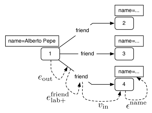
Figure 3: A single path along along the $f$ traversal.

The function $f$ says, traverse to the outgoing edges of vertex $i$, then only allow those edges with the label friend, then traverse to the incoming (i.e. head) vertices on those friend-labeled edges. Finally, of those vertices, return their name property. A single legal path according to this function is diagrammed in Figure 3. Though not diagrammed for the sake of clarity, the traversal would also go from vertex $1$ to the name of vertex $2$ and vertex $3$. The function $f$ is a “higher-order” adjacency defined as the composition of explicit adjacencies and serves as a join of Alberto and his friend’s names. The remainder of this section demonstrates graph traversals in real-world problems-solving situations.

3.1 Traversing for Recommendation

Recommendation systems are designed to help people deal with the problem of information overload by filtering information in the system that doesn’t pertain to the person rec:perugini2004 . In a positive sense, recommendation systems focus a person’s attention on those resources that are likely to be most relevant to their particular situation. There is a standard dichotomy in recommendation research—that of content- vs. collaborative filtering-based recommendation. The prior deals with recommending resources that share characteristics (i.e. content) with a set of resources. The latter is concerned with determining the similarity of resources based upon the similarity of the taste of the people modeled within the system collab:herlocker2006 . These two seemingly different techniques to recommendation are conveniently solved using a graph database and two simple traversal techniques rec:mirza2003 ; griffen:spread2006 . Figure 4 presents a toy graph data set, where there exist a set of people, resources, and features related to each other by likes- and feature-labeled edges. This simple data set is used for the remaining examples of this subsection.

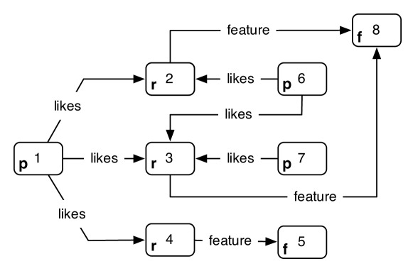
Figure 4: A graph data structure containing people (p), their liked resources (r), and each resource’s features (f).

Content-Based Recommendation

In order to identify resources that that are similar in features (i.e. content-based recommendation) to a resource, traverse to all resources that share the same features. This is accomplished with the following function, $f:\mathcal{\hat{P}}(V)\rightarrow\mathcal{\hat{P}}(V)$, where

$$f(i)=\left(\epsilon_{\epsilon-}^{i}\circ v_{\text{out}}\circ e_{\text{lab+}}^{\text{feature}}\circ e_{\text{in}}\circ v_{\text{in}}\circ e_{\text{lab+}}^{\text{feature}}\circ e_{\text{out}}\right)(i).$$

Assuming $i=3$, function $f$ states, traverse to the outgoing edges of resource vertex $3$, only allow feature-labeled edges, and then traverse to the incoming vertices of those feature-labeled edges. At this point, the traverser is at feature vertex $8$. Next, traverse to the incoming edges of feature vertex $8$, only allow feature-labeled edges, and then traverse to the outgoing vertices of these feature-labeled edges. At this point, the traverser is at resource vertices $3$ and $2$. However, since we are trying to identify those resources similar in content to vertex $3$, we need to filter out vertex $3$. This is accomplished by the last stage of the function composition. Thus, given the toy graph data set, vertex $2$ is similar to vertex $3$ in content. This traversal is diagrammed in Figure 5.

Figure 5: A traversal that identifies resources that are similar in content to a set of resources based upon shared features.

Its simple to extend content-based recommendation to problems such as: “Given what person $i$ likes, what other resources have similar features?” Such a problem is solved using the previous function $f$ defined above combined with a new composition that finds all the resources that person $i$ likes. Thus, if $g:\mathcal{\hat{P}}(V)\rightarrow\mathcal{\hat{P}}(V)$, where

$$g(i)=\left(v_{\text{in}}\circ e_{\text{lab+}}^{\text{likes}}\circ e_{\text{out}}\right)(i),$$

then to determine those resources similar in features to the resources that person vertex $7$ likes, compose function $f$ and $g$: $(f\circ g)(7)$. Those resources that share more features in common will be returned more by $f\circ g$.

What has been presented is an example of the use of traversals to do naïve content-based recommendation. It is possible to extend the functions presented to normalize paths (e.g. a resource can have every feature and thus, is related to everything), find novelty (e.g. feature paths that are rare and only shared by a certain subset of resources), etc. In most cases, when creating a graph traversal, a developer will compose different predefined paths into a longer compositions. Along with speed of execution, this is one of the benefits of using a functional, flow-based model for graph traversals graphflow:yoo2009 . Moreover, each component has a high-level meaning (e.g. the resources that a person likes) and as such, the verbosity of longer compositions can be minimal (e.g. $f\circ g$).

Collaborative Filtering-Based Recommendation

With collaborative filtering, the objective is to identify a set of resources that have a high probability of being liked by a person based upon identifying other people in the system that enjoy similar likes. For example, if person $a$ and person $b$ share 90% of their liked resources in common, then the remaining 10% they don’t share in common are candidates for recommendation. Solving the problem of collaborative filtering using graph traversals can be accomplished with the following traversal. For the sake of clarity, the traversal is broken into two components: $f$ and $g$, where $f:\mathcal{\hat{P}}(V)\rightarrow\mathcal{\hat{P}}(V)$ and $g:\mathcal{\hat{P}}(V)\rightarrow\mathcal{\hat{P}}(V)$.

$$f(i)=\left(\epsilon_{\epsilon-}^{i}\circ v_{\text{out}}\circ e_{\text{lab+}}^{\text{like}}\circ e_{\text{in}}\circ v_{\text{in}}\circ e_{\text{lab+}}^{\text{like}}\circ e_{\text{out}}\right)(i).$$

Function $f$ traverses to all those people vertices that like the same resources as person vertex $i$ and who themselves are not vertex $i$ (as a person is obviously similar to themselves and thus, doesn’t contribute anything to the computation). The more resources liked that a person shares in common with $i$, the more traversers will be located at that person’s vertex. In other words, if person $i$ and person $j$ share $10$ liked resources in common, then $f(i)$ will return person $j$ $10$ times. Next, function $g$ is defined as

$$g(j)=\left(v_{\text{in}}\circ e_{\text{lab+}}^{\text{like}}\circ e_{\text{out}}\right)(j).$$

Function $g$ traverses to all the resources liked by vertex $j$. In composition, $(g\circ f)(i)$ determines all those resources that are liked by those people that have similar tastes to vertex $i$. If person $j$ likes $10$ resources in common with person $i$, then the resources that person $j$ likes will be returned at least $10$ times by $g\circ f$ (perhaps more if a path exists to those resources from another person vertex as well). Figure 6 diagrams a function path starting from vertex $7$. Only one legal path is presented for the sake of diagram clarity.

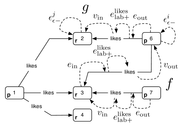
Figure 6: A traversal that identifies resources that are similar in content to a resource based upon shared features.

With the graph traversal pattern, there exists a single graph data structure that can be traversed in different ways to expose different types of recommendations—generally, different types of relationships between vertices. Being able to mix and match the types of traversals executed alters the semantics of the final rankings and conveniently allows for hybrid recommendation algorithms to emerge.

3.2 Traversing Endogenous Indices

A graph is a general-purpose data structure. A graph can be used to model lists, maps, trees, etc. As such, a graph can model an index. It was assumed, in §2.2, that a graph database makes use of an external indexing system to index the properties of its vertices and edges. The reason stated was that specialized indexing systems are better suited for special-purpose queries such as those involving full-text search. However, in many cases, there is nothing that prevents the representation of an index within the graph itself—vertices and edges can be indexed by other vertices and edges. In fact, given the nature of how vertices and edges directly reference each other in a graph database, index look-up speeds are comparable. Endogenous indices afford graph databases a great flexibility in modeling a domain. Not only can objects and their relationships be modeled (e.g. people and their friendships), but also the indices that partition the objects into meaningful subsets (e.g. people within a 2D region of space). The remainder of this subsection will discuss the representation and traversal of a spatial, 2D-index that is explicitly modeled within a property graph.

The domain of spatial analysis makes use of advanced indexing structures such as the quadtree quadtree:finkel1974 ; multi:samet2006 . Quadtrees partition a two-dimensional plane into rectangular boxes based upon the spatial density of the points being indexed. Figure 7 diagrams how space is partitioned as the density of points increases within a region of the index.

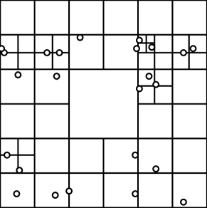
Figure 7: A quadtree partition of a plane. This figure is an adaptation of a public domain image provided courtesy of David Eppstein.

In order to demonstrate how a quadtree index can be represented and traversed, a toy graph data set is presented. This data set is diagrammed in Figure 8.

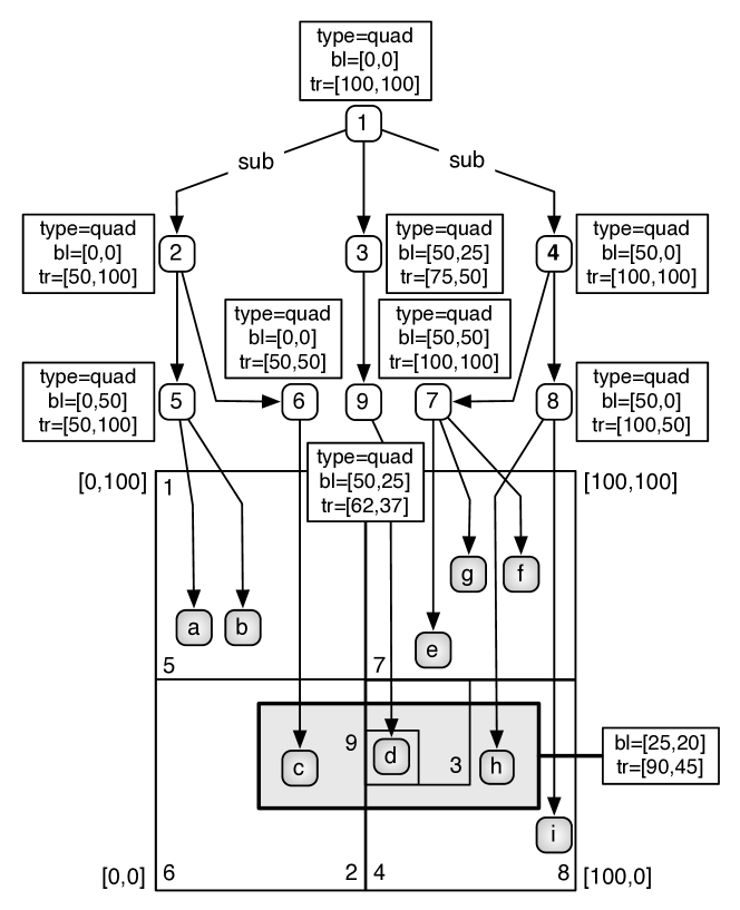
Figure 8: A quadtree index of a space that contains points of interest. The index is composed of the vertices $1$-$9$ and the points of interest are the vertices $a$-$i$. While not diagrammed for the sake of clarity, all edges are labeled sub (meaning subsumes) and each point of interest vertex has an associated bottom-left (bl) property, top-right (tr) property, and a type property which is equal to “poi.”

The top half of Figure 8 represents a quadtree index (vertices $1$-$9$). This quadtree index is partitioning “points of interest” (vertices $a$-$i$) located within the diagrammed plane. All vertices maintain three properties—bottom-left (bl), top-right (tr), and type. For a quadtree vertex, these properties identify the two corner points defining a rectangular bounding box (i.e. the region that the quadtree vertex is indexing) and the vertex type which is equal to “quad”. For a point of interest vertex, these properties denote the region of space that the point of interest exists within and the vertex type which is equal to “poi.”

Quadtree vertex $1$ denotes the entire region of space being indexed. This region is defined by its bottom-left (bl) and top-right (tr) corner points—namely $[0,0]$ and $[100,100]$, where $\text{bl}_{x}=0$, $\text{bl}_{y}=0$, $\text{tr}_{x}=100$, and $\text{tr}_{y}=100$. Within the region defined by vertex $1$, there are $8$ other defined regions that partition that space into smaller spaces (vertices $2$-$9$). When one vertex subsumes another vertex by a directed edge labeled sub (i.e. subsumes), the outgoing (i.e. tail) vertex is subsuming the space that is defined by the incoming (i.e. head) vertex. Given these properties and edges, identifying point of interest vertices within a region of space is simply a matter of traversing the quadtree index in a directed/algorithmic fashion.

In Figure 8, the shaded region represents the spatial query: “Which points of interest are within the rectangular region defined by the corner points $\text{bl}=[25,20]$ and $\text{tr}=[90,45]$?” In order to locate all the points of interest in this region, iteratively execute the following traversal starting from the root of the quadtree index (i.e. vertex $1$). The function is defined as $f:\mathcal{\hat{P}}(V)\rightarrow\mathcal{\hat{P}}(V)$, where

$$f(i)=\left(\epsilon_{\text{p+}}^{\text{tr}_{y}\geq 20}\circ\epsilon_{\text{p+}}^{\text{tr}_{x}\geq 25}\circ\epsilon_{\text{p+}}^{\text{bl}_{y}\leq 45}\circ\epsilon_{\text{p+}}^{\text{bl}_{x}\leq 90}\circ v_{\text{in}}\circ e_{\text{lab+}}^{\text{sub}}\circ e_{\text{out}}\right)(i).$$

The defining aspect of $f$ is the set of 4 $\epsilon_{\text{p+}}$ filters that determine whether the current vertex is overlapping or within the query rectangle. Those vertices not overlapping or within the query rectangle are not traversed to. Thus, as the traversal iterates, fewer and fewer paths are examined and the resulting point of interest vertices within the query rectangle are converged upon. With respect to Figure 8, after 3 iterations of $f$, the traversal will have returned all the points of interest within the query rectangle. The first iteration, will traverse to the index vertices 2, 3, and 4. The second iteration will traverse to the vertices 6, 8 and 9. Note that vertices 5 and 7 do not meet the criteria of the $\epsilon_{\text{p+}}$ filters. Finally, on the third iteration, the traversal returns vertices $c$, $d$, and $h$. Note that vertex $i$ is not returned because it, like 5 and 7, does not meet the $\epsilon_{\text{p+}}$ filter criteria. A summary of the legal vertices traversed to at each iteration is enumerate below.

1. 2, 3, 4

2. 6, 9, 8

3. $c$, $d$, $h$

There is a more efficient traversal that can be evaluated. If the bounding box defined by a quadtree vertex is completely subsumed by the query rectangle (i.e. not just overlapping), then, at that branch in the traversal, the traverser no longer needs to evaluate the $\epsilon_{\text{p+}}$-region filters and, as such, can simply iterate all the way down sub-labeled edges to the point of interest vertices knowing that they are completely within the query rectangle. For example, in Figure 8, once it is realized that vertex 9 is completely within the query rectangle, then the location properties of vertex $d$ do not need to be examined. The functions that define this traversal and the composition of these functions into a flow graph is defined below, where $A\subset\mathcal{\hat{P}}(V)$ is the multiset of all quadtree index vertices overlapping or within the query rectangle, $B\subseteq A$ is the multiset of all quadtree index vertices completely within the query rectangle, and $C\subset\mathcal{\hat{P}}(V)$ is the multiset of all point of interest vertices overlapping or within the query rectangle.

$$f(i) = \left(\epsilon_{\text{p+}}^{\text{tr}_{y}\geq 20}\circ\epsilon_{\text{p+}}^{\text{tr}_{x}\geq 25}\circ\epsilon_{\text{p+}}^{\text{bl}_{y}\leq 45}\circ\epsilon_{\text{p+}}^{\text{bl}_{x}\leq 90}\circ\epsilon_{\text{p+}}^{\text{type}=\text{quad}}\circ v_{\text{in}}\circ e_{\text{lab+}}^{\text{sub}}\circ e_{\text{out}}\right)(i)$$

$$g(i) = \left(\epsilon_{\text{p+}}^{\text{tr}_{y}\leq 45}\circ\epsilon_{\text{p+}}^{\text{tr}_{x}\leq 90}\circ\epsilon_{\text{p+}}^{\text{bl}_{y}\geq 20}\circ\epsilon_{\text{p+}}^{\text{bl}_{x}\geq 25}\right)(i)$$

$$h(i) = \left(\epsilon_{\text{p+}}^{\text{type}=\text{quad}}\circ v_{\text{in}}\circ e_{\text{lab+}}^{\text{sub}}\circ e_{\text{out}}\right)(i)$$

$$s(i) = \left(\epsilon_{\text{p+}}^{\text{tr}_{y}\geq 20}\circ\epsilon_{\text{p+}}^{\text{tr}_{x}\geq 25}\circ\epsilon_{\text{p+}}^{\text{bl}_{y}\leq 45}\circ\epsilon_{\text{p+}}^{\text{bl}_{x}\leq 90}\circ\epsilon_{\text{p+}}^{\text{type}=\text{poi}}\circ v_{\text{in}}\circ e_{\text{lab+}}^{\text{sub}}\circ e_{\text{out}}\right)(i)$$

$$r(i) = \left(\epsilon_{\text{p+}}^{\text{type}=\text{poi}}\circ v_{\text{in}}\circ e_{\text{lab+}}^{\text{sub}}\circ e_{\text{out}}\right)(i)$$

Function $f$ traverses to those quadtree vertices that overlap or are within the query rectangle. Function $g$ allows only those quadtree vertices that are completely within the query rectangle. Function $h$ traverses to subsumed quadtree vertices. Function $s$ traverses to point of interest vertices that are overlapping or within the query rectangle. Finally, function $r$ traverses to subsumed point of interest vertices. Note that functions $h$ and $r$ do no check the bounding box properties of their domain vertices. As a quadtree becomes large, this becomes a more efficient solution to finding all points of interest within a query rectangle.

The ability to model an index endogenous to a graph allows the domain modeler to represent not only objects and their relations (e.g. people and their friendships), but also “meta-objects” and their relationships (e.g. index nodes and their subsumptions). In this way, the domain modeler can organize their model according to partitions that make sense to how the model will be used to solve problems. Moreover, by combining the traversal of an index with the traversal of a domain, there exists a single unified means by which problems are solved within a graph database—the graph traversal pattern.

4 Conclusion

Graphs are a flexible modeling construct that can be used to model a domain and the indices that partition that domain into an efficient, searchable space. When the relations between the objects of the domain are seen as vertex partitions, then a graph is simply an index that relates vertices to vertices by edges. The way in which these vertices relate to each other determines which graph traversals are most efficient to execute and which problems can be solved by the graph data structure. Graph databases and the graph traversal pattern do not require a global analysis of data. For many problems, only local subsets of the graph need to be traversed to yield a solution. By structuring the graph in such a way as to minimize traversal steps, limit the use of external indices, and reduce the number of set-based operations, modelers gain great efficiency that is difficult to accomplish with other data management solutions.

References

- (1) Gary Chartrand and Linda Lesniak. Graphs & Digraphs. Wadsworth Publishing Company, Belmont, CA, 1986.
- (2) Edgar F. Codd. A relational model of data for large shared data banks. Communications of the ACM, 13(6):377–387, 1970.
- (3) Giuseppe DeCandia, Deniz Hastorun, Madan Jampani, Gunavardhan Kakulapati, Avinash Lakshman, Alex Pilchin, Swaminathan Sivasubramanian, Peter Vosshall, and Werner Vogels. Dynamo: Amazon’s highly available key-value store. SIGOPS Operating Systems Review, 41(6):205–220, 2007.
- (4) Raphael A. Finkel and J. L. Bentley. Quad trees a data structure for retrieval on composite keys. Acta Informatica, 4(1):1–9, March 1974.
- (5) Josephine Griffith, Colm O’Riordan, and Humphrey Sorensen. Knowledge-Based Intelligent Information and Engineering Systems, volume 4253 of Lecture Notes in Artificial Intelligence, chapter A Constrained Spreading Activation Approach to Collaborative Filtering, pages 766–773. Springer-Verlag, 2006.
- (6) Johnathan L. Herlocker, Joseph A. Konstan, Loren G. Terveen, and John T. Riedl. Evaluating collaborative filtering recommender systems. ACM Transactions on Information Systems, 22(1):5–53, 2004.
- (7) Patrik Larsson. Analyzing and adapting graph algorithms for large persistent graphs. Master’s thesis, Linköping University, 2008.
- (8) Joe Lennon. Beginning CouchDB. Apress, 2009.
- (9) Norbert Martínez-Bazan, Victor Muntés-Mulero, Sergio Gómez-Villamor, Jordi Nin, Mario-A. Sánchez-Martínez, and Josep-L. Larriba-Pey. DEX: high-performance exploration on large graphs for information retrieval. In Proceedings of the Sixteenth ACM Conference on Information and Knowledge Management, pages 573–582, New York, NY, 2007. ACM.
- (10) Batul J. Mirza, Benjamin J. Keller, and Naren Ramakrishnan. Studying recommendation algorithms by graph analysis. Journal of Intelligent Information Systems, 20(2):131–160, 2003.
- (11) Priti Mishra and Margaret H. Eich. Join processing in relational databases. ACM Computing Surveys, 24(1):63–111, 1992.
- (12) G. P. Monro. The concept of multiset. Mathematical Logic Quarterly, 33(2):171–178, 1987.
- (13) John Paul Morrison. Flow-Based Programming: A New Approach to Application Development. Van Nostrand Reinhold, 1994.
- (14) Saverio Perugini, Marcos Andre Goncalves, and Edward A. Fox. Recommender systems research: A connection-centric survey. Journal of Intelligent Information Systems, 23(2):107–143, 2004.
- (15) Marko A. Rodriguez. Mapping semantic networks to undirected networks. International Journal of Applied Mathematics and Computer Science, 5(1):39–42, February 2008.
- (16) Marko A. Rodriguez and Joshua Shinavier. Exposing multi-relational networks to single-relational network analysis algorithms. Journal of Informetrics, 4(1):29–41, 2009.
- (17) Hanan Samet. Foundations of Multidimensional and Metric Data Structures. Morgan Kaufmann, August 2006.
- (18) Michael Stonebraker. The case for shared nothing. IEEE Database Engineering Bulletin, 9(1):4–9, 1986.
- (19) Andy Yoo and Ian Kaplan. Evaluating use of data flow systems for large graph analysis. In Proceedings of the 2nd Workshop on Many-Task Computing on Grids and Supercomputers, pages 1–9, New York, NY, 2009. ACM.