A model independent null test on the cosmological constant
Abstract
We use the Om statistic and the Genetic Algorithms (GA) in order to derive a null test on the spatially flat cosmological constant model CDM. This is done in two steps: first, we apply the GA to the Constitution SNIa data in order to acquire a model independent reconstruction of the expansion history of the Universe and second, we use the reconstructed in conjunction with the Om statistic, which is constant only for the CDM model, to derive our constraints. We find that while CDM is consistent with the data at the level, some deviations from CDM model at low redshifts can be accommodated.
keywords:
cosmology: theory - (cosmology:) dark energy - (cosmology:) cosmological parameters.1 Introduction
In the previous decade it was discovered that the Universe is undergoing an accelerated expansion (Riess et al. 2004; Spergel et al. 2007; Readhead et al. 2004). This acceleration is usually attributed either to a cosmic fluid with negative pressure dubbed Dark Energy or to an IR modification of gravity. In order to identify the properties of Dark Energy or the structure of the IR modification of gravity it is necessary to know to a high precision the rate of the expansion of the Universe, parameterized as where is the scale factor and is the redshift of the cosmological probe, as it measured by the observations.
The behavior of the expansion of the Universe can be identified by studying two functions, the Equation of State (EoS) which can be rewritten as
| (1) |
where accounts for all terms in the Friedmann equation not related to matter and the deceleration parameter which can be rewritten as
| (2) |
Obviously, the cosmological constant () corresponds to a constant dark energy density, while in general can be time dependent. Also, an important parameter is the value of the deceleration parameter today, ie , which for the cosmological constant model in GR it is .
However, despite all the recent progress the origin of the accelerated expansion of the universe still remains unknown with many possibilities still remaining open, see for example Perivolaropoulos (2006). The simplest choice that agrees well with the data is a positive cosmological constant which has to be small enough to have started dominating the universe at late times. As it was demonstrated by the Seven-Year WMAP data (Komatsu et al. 2010), the cosmological constant remains the best candidate and has the advantage of having only one free parameter related to the properties of the Dark Energy. Nonetheless, this model fails to explain why the cosmological constant is so small that it can only dominate the universe at late times, a problem known as the coincidence problem and there are a few cosmological observations which differ from its predictions (Perivolaropoulos 2008; Perivolaropoulos & Shafieloo 2008).
A very important complication in the investigation of the behavior of dark energy occurs due to the bias introduced by the parameterizations used. At the moment, there is a multitude of available phenomenological ansätze for the dark energy equation of state parameter or dark energy density, each with its own merits and limitations (see Sahni & Starobinsky (2006) and references therein). The interpretation of the SNIa data has been shown to depend greatly on the type of parametrization used to perform a data fit (Sahni & Starobinsky 2006; Shafieloo, Sahni & Starobinsky 2009). Choosing a priori a model for dark energy can thus adversely affect the validity of the fitting method and lead to compromised or misleading results.
The need to counteract this problem paved the way for the consideration of a complementary set of non-parametric reconstruction techniques (Daly & Djorgovski 2003; Wang & Mukherjee 2004; Saini 2003; Wang 2009; Clarkson & Zunckel) and model independent approaches (Sahni et al. 2002; Alam et al. 2003; Shafieloo et al. 2006, Shafieloo 2007; Wang & Tegmark 2005; Shafieloo & Clarkson 2010). These try to minimize the ambiguity due to a possibly biased assumption for by fitting the original datasets without using any parameters related to some specific model. The result of these methods can then be interpreted in the context of a dark energy model of choice. Non-parametric reconstructions can thus corroborate parametric methods and provide more credibility. However, they too suffer from a different set of problems, mainly the need to resort to differentiation of noisy data, which can itself introduce great errors.
In this paper, we present a method that can be used as a model independent approach in testing the standard cosmological model. This is done by using the Genetic Algorithms (GA) technique, first used in the analysis of SNIa data in Bogdanos & Nesseris (2009). The GAs represent a method for non-parametric reconstruction of the dark energy equation of state parameter , based on the notions of genetic algorithms and grammatical evolution. GAs are more useful and efficient than usual techniques when
-
•
The parameter space is very large, too complex or not enough understood, as is the case with dark energy.
-
•
Domain knowledge is scarce or expert knowledge is difficult to encode to narrow the search space.
-
•
Traditional search methods give poor results or completely fail.
Naturally, therefore, they have been used with success in many fields where one of the above situations is encountered, like the computational science, engineering and economics. Recently, they have also been applied to study high energy physics (Becks, Hahn & Hemker 1994; Allanach, Grellscheid & Quevedo 2004; Rojo & Latorre 2004) gravitational wave detection (Crowder, Cornish & Reddinger 2006) and gravitational lensing (Brewer & Lewis 2005). Since the nature of Dark Energy still remains a mystery, this makes it for us an ideal candidate to use the GAs as a means to analyze the SNIa data and extract model independent constraints on the behavior of the Dark Energy. In Section 2 we briefly describe the Om statistic while in Section 3 we provide an overview of the general methodology of the GA paradigm and finally, we present our results in Section 4.
2 The Om statistic
The recently introduced diagnostic (Sahni, Shafieloo & Starobinsky 2008) (also look at Zunckel & Clarkson (2008)) enables us to distinguish CDM from other dark energy models without directly involving the cosmic EOS. The diagnostic is defined as:
| (3) |
For dark energy with a constant equation of state ,
| (4) |
(we assume that the universe is spatially flat for simplicity). Consequently,
| (5) |

from where we find in CDM, whereas in quintessence while in phantom . We therefore conclude that: if dark energy is a cosmological constant. Note that since in CDM, this model contains SCDM as an important limiting case. Consequently the diagnostic cannot distinguish between large and small values of the cosmological constant unless the value of the matter density is independently known. In other words, the diagnostic provides us with a null test of the cosmological constant. This is a simple consequence of the fact that plotted against results in a straight line for CDM, whose slope is given by . For other dark energy models the line describing is curved, since the equality
| (6) |
(which always holds for CDM for any ) is satisfied in quintessence/phantom type models only at redshifts significantly greater than unity, when the effects of dark energy on the expansion rate can safely be ignored. As a result the efficiency of the diagnostic improves at low redshifts () precisely where there is likely to be an abundance of cosmological data in the coming years!
For a constant EoS: at , consequently a larger is indicative of a larger ; while at high , , as shown in Fig. 1.
On the other hand, for quintessence as well as phantom the line describing is curved, which helps distinguish these models from CDM even if the value of the matter density is not accurately known – see Fig. 1.
In practice, the construction of requires a knowledge of the Hubble parameter, , which can be determined using a number of model independent approaches (Sahni et al. 2003; Alam et al. 2003; Shafieloo et al. 2006, Shafieloo 2007; Wang & Tegmark 2005; Shafieloo & Clarkson 2010).
3 Genetic algorithms
3.1 Overview
GAs were introduced as a computational analogy of adaptive systems. They are modelled loosely on the principles of the evolution via natural selection, employing a population of individuals that undergo selection in the presence of variation-inducing operators such as mutation and crossover. The encoding of the chromosomes is called the genome or genotype and is composed, in loose correspondence to actual DNA genomes, by a series of representative “genes”. Depending on the problem, the genome can be a series (vector) of binary numbers, decimal integers, machine precision integers or reals or more complex data structures.
In order to evaluate the individual chromosomes a fitness function is used and reproductive success usually varies with fitness. The fitness function is a map between the gene sequence of the chromosomes (genotype) and a number of attributes (phenotype), directly related to the properties of a wanted solution. Often the fitness function is used to determine a “distance” of a candidate solution from the true one. Various distance measures can be used for this purpose (Euclidean distance, Manhattan, Mahalanobis etc.).
The algorithm begins with an initial population of candidate solutions, which is usually randomly generated. Although GA’s are relatively insensitive to initial conditions, i.e. the population we start from is not very significant, but using some prescription for producing this seed generation can affect the speed of convergence. In each successive step, the fitness functions for the chromosomes of the population are evaluated and a number of genetic operators (mutation and crossover) are applied to produce the next generation. This process continues until some termination criteria is reached, e.g. obtain a solution with fitness greater than some predefined threshold or reach a maximum number of generations. The later is imposed as a condition to ensure that the algorithm terminates even if we cannot get the desired level of fitness.
The various steps of the algorithm can be summarized as follows:
-
1.
Randomly generate an initial population
-
2.
Compute and save the fitness for each individual m in the current population .
-
3.
Define selection probabilities for each individual in so that is proportional to the fitness.
-
4.
Generate by probabilistically selecting individuals from to produce offspring via genetic operators (crossover and mutation).
-
5.
Repeat step 2 until a satisfying solution is obtained, or a maximum number of generations reached.
We should stress that the initial population will only depend on the choice of the grammar and therefore it can only affect on how fast the algorithm will converge to the minimum. Using the wrong grammar may result in the GA being trapped in a local minimum. Also, two important parameters that affect the transition from the population to are the selection rate and the mutation rate. The selection rate is typically of the order of and it affects how many of the individuals, after they are ranked with respect to their fitness, will be allowed to produce offspring. The mutation rate is usually of the order of and it expresses the probability that an arbitrary part of the genetic sequence will be changed from its previous state. This is done in order to maintain the genetic diversity from one generation of a population to the next.
The paradigm of GAs described above is usually the one applied to solving most of the problems presented to GAs. Though it might not find the best solution, more often than not, it would come up with a partially optimal solution. A more detailed overview and its application in cosmology can be found in Bogdanos & Nesseris (2009).
The difference of the GA over the the standard analysis of the data, ie having an a priori defined model with some free parameters, is that the obtained values of the best-fit parameters are model-dependent and in general models with more parameters tend to give better fits to the data. This is where the GA approach starts to depart from the ordinary parametric method. Our goal is to minimize a function, not using a candidate model function for the distance modulus and varying parameters, but through a stochastic process based on a GA evolution. This way, no prior knowledge of a dark energy model is needed to obtain a solution and our result will be completely parameter-free.
In simpler terms, the GA method does not require an a priori assumption for a DE model, but uses the data themselves to find this model. Also, it is parameter free as the end result does not have any free parameters that can be changed in order to fit the data. So, in this sense this method has far less bias any of the standard methods for the reconstruction of the expansion history of the Universe. This is the main reason for the use of the GAs in this paper.
3.2 General Methodology
We first outline the course of action we follow to apply the GA paradigm in the case of SNIa data. For the application of GA and grammatical evolution (GE) on the dataset, we use a modified version of the GDF (Tsoulos et al. 2006) tool 111http://cpc.cs.qub.ac.uk/summaries/ADXC, which uses GE as a method to fit datasets of arbitrary size and dimensionality. This program uses the tournament selection method for crossover. GDF requires a set of input data (train set), an (optional) test sample and a grammar to be used for the generation of functional expressions. The output is an expression for the function which best fits the train set data.
Since the SNIa datapoints are given in terms of the distance modulus , the fitness function for the GA we have chosen is equal to , where
| (7) |
where for the Constitution set and are the errors due to flux uncertainties, intrinsic dispersion of SNIa absolute magnitude and peculiar velocity dispersion and is the reduced distance modulus obtained for each chromosome of the population by the GA.
An advantage of our method is the fact that neither the nor the depend on any parameters. Also, as it can be seen from eq. (7), our method does not make an assumption of flatness or not in order to fit the data. Flatness (or non-flatness) only comes into play when one tries to find the luminosity distance and the underlying dark energy model given the best-fit form of . So, in this aspect the result produced by the GA is independent of the assumption of flatness as well.
The GA evaluates (7) in each evolutionary step for every chromosome of the population. The one with the best fitness will consequently have the smallest and will be the best candidate solution in its generation. Of all the steps in the execution of the algorithm, the evaluation of the fitness is the most expensive. GDF is appropriately modified to use (7) as the basis of its fitness calculation.
After the execution of the GA, we obtain an expression for the reduced distance modulus as the solution of best fitness and the corresponding . Using this we can, through differentiation, obtain other functions or parameters of interest, such as the Om statistic or the deceleration parameter . For example, for a flat Universe the Hubble parameter will be given by
| (8) |
and then the deceleration parameter can be found by Eq. (2).
A possible complication of this method is that it gives no direct way to estimate the errors for the derived parameters. One cannot expect to get an estimate by just running the algorithm many times and obtaining slightly different parameters. The GA usually tends to converge at the same solution for a given dataset, unless we change significantly the population size or the number of generations. A way to circumvent this problem is to use a bootstrap Monte Carlo simulation to produce synthetic datasets and rerun the algorithm on them. We can thus obtain a statistical sample of parameter values which will allow us to estimate the error.
We sketch the procedure we will follow Press et al. (1992):
-
1.
The GA is applied on the original SNIa dataset with the chosen execution parameters and a solution for is obtained.
-
2.
Generate a number of synthetic datasets by drawing each time the same number of data points with replacement from the original set.
-
3.
The GA is rerun for the synthetic datasets.
-
4.
A new set of values for the Om statistic and the deceleration parameter is generated.
-
5.
The error of the desired parameter can be found by taking the 2.5 and the 97.5 percentiles of the bootstrap distribution (Efron 1982).
Using the above steps, we can obtain error estimates for any desired parameter.
3.3 An example
In this Section we will briefly describe a simple example222This is only a schematic description of how the GA works and this is done solely for the sake of explaining the basic mechanisms of the GA. of how he GA determines the best-fit. We will avoid describing the technicalities, like the binary representation of the solutions, and instead we will concentrate on how the generations evolve, how many and which individuals are chosen for the next generation etc.
As we mentioned earlier, the choice of the grammar is very important, however in order to keep our example as simple as possible we will assume that our grammar includes only basic functions like polynomials , etc, the trigonometric functions , , the exponential and the logarithm .
The first step in the GA is setting up a random initial population which can be any simple combination of these functions, eg , and . The number of number of candidate solutions (chromosomes) in the genetic population is usually a few hundreds and later on we will use the value of 500.
Next, the algorithm measures the fitness of each solution by calculating their , ie for our simple example , and . The selection per se is done by implementing the “Tournament selection” method which involves running several “tournaments”, sorting the population with respect to the fitness each individual and after that a fixed percentage, adjusted by the selection rate (see the previous subsection), of the population is chosen. As we mentioned, the selection rate is of the order of of the total population, but lets assume that the two out of the three candidate solutions ( and ) are chosen for the sake of simplicity.
The reproduction of these two solutions will be done by the crossover and mutation operations. The crossover will randomly combine parts of the “parent” solutions, for example in one such realization this may be schematically shown as
After this is done, the GA will proceed to implement the mutation operation. The probability for mutation is adjusted by the mutation rate, which as we mentioned is typically of the order of . In our example this may be a change in the power of some term or the change in the value of a coefficient. For example, for the candidate solution this can be schematically shown as , where the power of the term was mutated from to .
Finally, at the end of the first round we have the three candidate solutions
At the beginning of the next round the fitness of each individual will again be determined, which for our population will be , and the selection and the other operations will proceed as before. It is easily seen that even after one generation the of the candidate solutions has decreased dramatically and as we will see in the next section, it only takes a bit more than 100 generations to reach an acceptable and about 500 to 1000 generations to start converging on the minimum.
After a predetermined number of generations, usually on the order of , has been reached or some other criteria have been met, the GA will finish, with the best candidate solution of the last generation being the best-fit to the data.
4 Results
We will now examine a number of different configurations, highlighted in Table 1. In order to keep our analysis as simple as possible we will use a Basic Grammar that includes polynomials like , etc, the trigonometric functions , , the exponential and the logarithm and a second grammar that includes the Basic Grammar and the Legendre polynomials. For the analysis we will use the Constitution SNIa dataset of Hicken et al. (2009) consisting of 397 SNIa. The steps followed for the usual minimization of (7) in terms of its parameters are described in detail in Nesseris & Perivolaropoulos (2004); Nesseris & Perivolaropoulos (2005); Lazkoz, Nesseris & Perivolaropoulos (2005), Nesseris & Perivolaropoulos (2007).
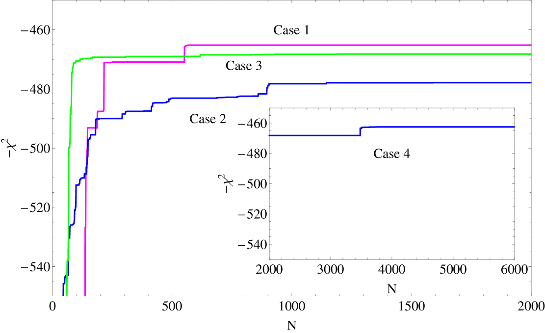
In Fig. 2 we show the fitness (equal to ) as a function of the number of generations. Clearly, all configurations seem to have to have converged very early or to be very close to converging to their minimum. An exception is Case 3 which even after 3000 generations still has not converged and we had to run the simulation for another 3000 generations to check its convergence. Since we want to compare the configurations with equal standards, ie number of generations etc, we will treat this case (Case 4) separately.
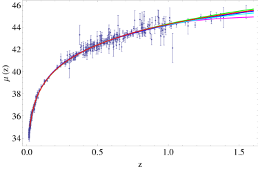
As it can be seen from Table 1 and Fig. 3, most configurations agree well with the data and actually have a minimum comparable or even better with respect to CDM. An exception to this is Case 2, where the best fit differs from CDM by a thus providing a much poorer fit. The reason for this is the fact that by increasing the grammar we effectively increase the landscape in which the algorithm has to search and therefore, we are making the fit poorer as the GA will take much much longer to converge.
| Case 1 | Basic grammar | |
| Case 2 | Basic grammar + Legendre polyn. | |
| Case 3 | Only polyn. in grammar (3000 gen.) | |
| Case 4 | Only polyn. in grammar (6000 gen.) | |
| CDM |
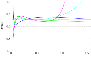
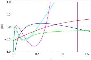
In Figs. 4 and 5 we show the corresponding results of each case for the Om statistic and the deceleration parameter (our best-fit function corresponds to the cyan line). Due to the presence of trigonometric functions into the best fit and the fact that the Om statistic is derived from the Hubble parameter by differentiation, Case 1 exhibits strong oscillations. This is also apparent in the corresponding plot for the deceleration parameter for Case 2 (magenta line, Fig. 5).
As it can be seen in Fig. 1, a constant (but different from ) forces the Om statistic to be a monotonic function that is located completely either above or below the constant case (). However, none of the curves in Fig. 4 are monotonic functions and all of them cross the constant Om case several times. Also, all cases remain reasonably close to the CDM value of for intermediate redshifts but deviate from that value at high or low redshifts. Therefore, this could be the effect of a time-dependent equation of state instead of a constant . Comparing with Fig. 1, it is possible that this behaviour is due to an equation of state more negative than -1.
This is also supported from Fig. 4 and Fig. 5 as at low redshifts all cases predict a much different forms of acceleration than the best fit CDM. In Fig. 4 and Fig. 5 our best fit results show an overall slowing down of the acceleration at the low redshifts (which is in concordance with results presented in Shafieloo et al. (2009) with a very rapid increase of acceleration at the very low redshifts. These are very similar with the results presented in Fig.2 of Shafieloo & Clarkson (2010) where smoothing method of reconstruction of the expansion history of the universe is being used. It is obvious that when two very different model independent approaches reach to a similar result, we must be on the right track and very close to the best possible result. However, theoretical interpretation of these results is beyond the scope of this paper. In fact there might be very different mechanisms that result to a similar expansion history of the universe as we reconstructed in this paper (e.g see Csaki, Kaloper, and Terning (2002); Alam et al. (2003), Kelly et al. (2010); Sullivan et al. (2010)).
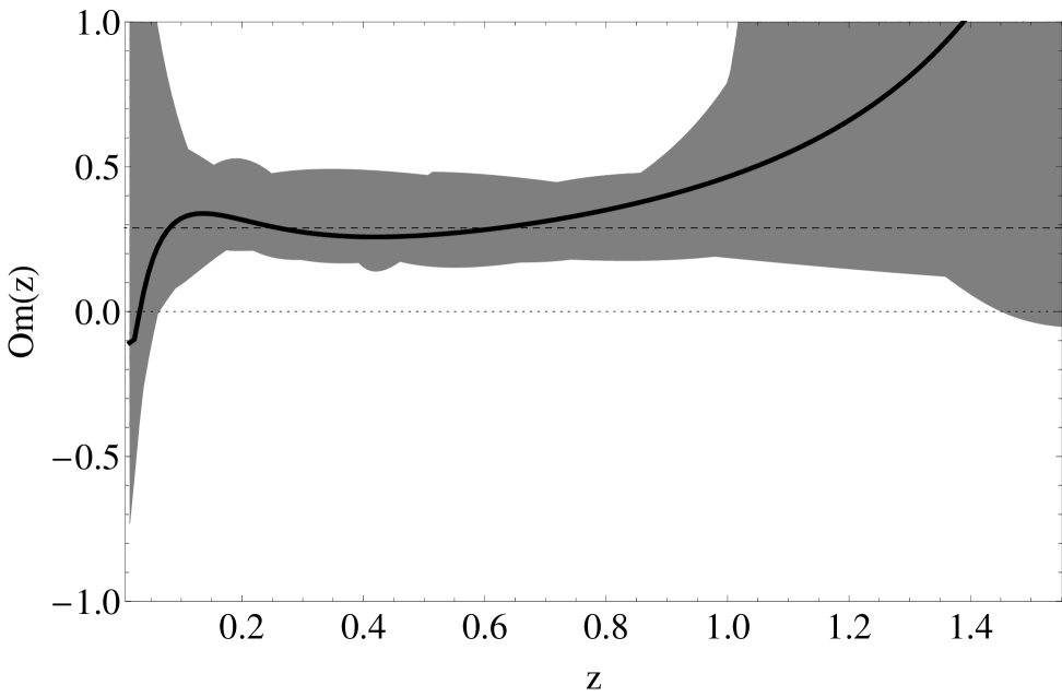
In Fig. 6 we show the Om statistic as a function of the redshift . The black line corresponds to the best fit of case 4, while the gray-shaded area to the error region. The error region was calculated by implementing a bootstrap monte-carlo simulation as discussed in the previous section. Note that the overall slowing down of the acceleration at the low redshifts cannot be clearly seen from this figure as the errors are quite symmetrical around the best fit CDM value. However, as we mentioned earlier this is clearly seen by the behavior of the deceleration parameter in Fig. 5.
As it can be seen in Fig. 6, CDM remains consistent with the data at the level but at the same time, some deviations from the standard CDM model can be accommodated. Due to the large errorbars of the current datasets, many dark energy models are still consistent with them but we expect this to change in the near future with the advent of high quality SnIa observations.
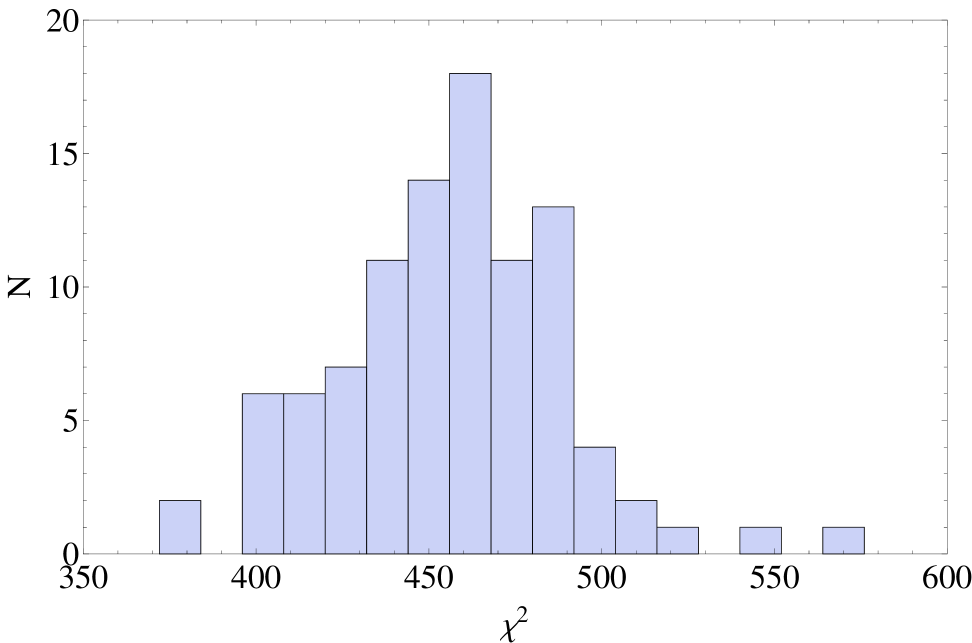
In Fig. 7 we show a histogram of the bootstrap distribution found from the monte-carlo simulation that was used to create the error regions. Clearly, the distribution is quite symmetrical and centered, so we are confident that our error region in Fig. 6 was correctly reconstructed. Finally, we also tested the GA on a mock CDM dataset and we found that it can reconstruct the luminosity distance curve to within , so we are confident that is does not overfit the data, but instead it can successfully detect the underlying DE model.
5 Conclusions
We used the Om statistic and the GAs in order to derive a null test on the cosmological constant model CDM. Our interest in the GAs stems from the fact that they represent a method for non-parametric reconstruction of the expansion history of the universe, based on the notions of genetic algorithms and grammatical evolution. These kinds of algorithms are more useful and efficient than usual techniques especially when the problem under examination is not well understood, as is the case with dark energy. Since the nature of dark energy still remains a mystery, this makes it for us an ideal candidate to use the GAs as a means to analyze the SNIa data and extract model independent constraints on the behavior of the Dark Energy. On the other hand, the diagnostic (Sahni et al. 2008) enables us to distinguish CDM from other dark energy models without directly involving the cosmic EoS.
Our methodology is completely model independent and it can be summarized in two steps: first, we applied the GA to the Constitution SNIa data in order to acquire a model independent reconstruction of the expansion history of the Universe . After we reconstructed , the second step was to use it in conjunction with the Om statistic and derive our null test.
Our main results was that CDM remains consistent with the data at the level, see Fig. 6, but at the same time, some deviations from the standard CDM model can be accommodated and this is also in accordance with the data especially at low redshifts (see the behavior of the best fit in Fig. 6).
However, we should mention that the slowing down at low redshifts for the Constitution set mentioned earlier can also be seen with the standard analysis with the CPL ansatz (see Sanchez, Nesseris & Perivolaropoulos (2009)) but only for the Constitution set. For the other SNIa datasets the reverse trend (speeding up the acceleration at low z) was observed. For this reason and due to the fact that the current data still have quite large errors we believe that the full potential of our method, while it is very promising, will only be realized in the near future when more high quality SNIa data will become available. When this happens, the error region at low in Fig. 6 will be small enough for the Om statistic to completely discriminate between CDM and the various Dark Energy models.
Acknowledgements
The authors acknowledge use of the GDF program. The source code is freely available from http://cpc.cs.qub.ac.uk/summaries/ADXC. The authors would like to thank L. Perivolaropoulos and an anonymous referee for very useful comments on the manuscript. S.N. would like to thank C. Bogdanos for very fruitful discussions and the Laboratoire de Physique Theorique (LPT) in Orsay for the warm hospitality during his stay there. S.N. is supported by the Niels Bohr International Academy, the Danish Research Council under FNU Grant No. 272-08-0285 and the DISCOVERY center. A.S. acknowledges the support of the EU FP6 Marie Curie Research and Training Network “UniverseNet” (MRTN-CT-2006-035863). A.S. would like to thank the Niels Bohr International Academy and DISCOVERY Center where part of this work was undertaken.
References
- [1] Allanach B. C. ,Grellscheid D., Quevedo F. , 2004, JHEP, 0407, 069, [arXiv:hep-ph/0406277].
- [2] Alam U. , Sahni V. , Starobinsky A. A. , 2003, JCAP, 0304, 002
- [3] Becks K. H. ,Hahn S., Hemker A. , 1994, Phys. Bl. 50, 238;
- [4] Bogdanos C., Nesseris S. , 2009, JCAP 0905, 006, [arXiv:0903.2805 [astro-ph.CO]].
- [5] Brewer B. J. , Lewis G. F. , 2005, arXiv:astro-ph/0501202.
- [6] Clarkson C., Zunckel C. , 2010, arXiv:1002.5004.
- [7] Crowder J. ,Cornish N. J., Reddinger L. , 2006, Phys. Rev. D ,73, 063011, [arXiv:gr-qc/0601036].
- [8] Csaki C. , Kaloper N. , Terning J. , 2002, Phys. Rev. Lett, 88, 161302
- [9] Daly R. A., Djorgovski S. G. , 2003, ApJ, 597, 9, [arXiv:astro-ph/0305197].
- [10] Efron B. , 1982, Society of Industrial and Applied Mathematics, CBMS-NSF Monographs 38.
- [11] Hicken M. et al., 2009, ApJ, 700, 1097, [arXiv:0901.4804 [astro-ph.CO]].
- [12] Kelly P. et al., 2010, ApJ., 715, 743 (2009) [arXiv:0912.0929 ].
- [13] Komatsu E. et al., 2010, arXiv:1001.4538.
- [14] Lazkoz R., Nesseris S., Perivolaropoulos L. , 2005, JCAP 0511, 010, [arXiv:astro-ph/0503230].
- [15] Nesseris S., Perivolaropoulos L., 2004, Phys. Rev. D 70, 043531, [arXiv:astro-ph/0401556].
- [16] Nesseris S., Perivolaropoulos L., 2005, Phys. Rev. D 72, 123519, [arXiv:astro-ph/0511040].
- [17] Nesseris S., Perivolaropoulos L., 2007, JCAP 0701, 018 [arXiv:astro-ph/0610092].
- [18] Perivolaropoulos L., 2006, AIP Conf. Proc. 848, 698, [arXiv:astro-ph/0601014].
- [19] Perivolaropoulos L., 2008, arXiv:0811.4684 [astro-ph].
- [20] Perivolaropoulos L., Shafieloo A., 2008, arXiv:0811.2802 [astro-ph].
- [21] Press W. H. et. al., 1994, ‘Numerical Recipes’, Cambridge University Press.
- [22] Readhead A. C. S. et al., 2004, ApJ., 609, 498, [arXiv: astro-ph/0402359].
- [23] Riess A. G. et al. [Supernova Search Team Collaboration], 2004, ApJ, 607, 665.
- [24] Rojo J., Latorre J. I., 2004, JHEP 0401, 055, [arXiv:hep-ph/0401047];
- [25] Sahni V., Starobinsky A. , 2006, Int. J. Mod. Phys. D 15, 2105, [arXiv:astro-ph/0610026].
- [26] Sahni V., Saini T. D., Starobinsky A. A., Alam U. , 2003, JETP Lett. 77, 201 [Pisma Zh. Eksp. Teor. Fiz. 77, 249], [arXiv:astro-ph/0201498].
- [27] Sahni V., Shafieloo A., Starobinsky A. A. , Phys. Rev. D 78, 103502 (2008) [arXiv:0807.3548 [astro-ph]].
- [28] Saini T. D., 2003, MNRAS., 344, 129 [arXiv:astro-ph/0302291].
- [29] Sanchez J. C. B. , Nesseris S. , Perivolaropoulos L., 2009, JCAP 0911, 029, [arXiv:0908.2636 [astro-ph.CO]].
- [30] Shafieloo A., 2007, MNRAS, 380, 1573, [arXiv:astro-ph/0703034].
- [31] Shafieloo A., Alam U.,Sahni V., Starobinsky A. A., 2006, MNRAS, 366, 1081, [arXiv:astro-ph/0505329].
- [32] Shafieloo A., Clarkson C., 2010, Phys. Rev. D 81, 083537, [arXiv:0911.4858 [astro-ph.CO]].
- [33] Shafieloo A., Sahni V., Starobinsky A. A., 2009, Phys. Rev. D 80, 101301, [arXiv:0903.5141 [astro-ph.CO]].
- [34] Spergel D. N. et al. [WMAP Collaboration], 2007, ApJ.Sup., 170, 377, [arXiv:astro-ph/0603449].
- [35] Sullivan M. et al., 2010, arXiv:1003.5119
- [36] Tsoulos I.G., Gavrilis D., Dermatas E., 2006, Computer Physics Communications 174, 555-559.
- [37] Wang Y., 2009, Phys. Rev. D 80, 123525, [arXiv:0910.2492].
- [38] Wang Y., Mukherjee P., 2004, ApJ., 606, 654, [arXiv:astro-ph/0312192].
- [39] Wang Y., Tegmark M., 2005, Phys. Rev. D 71, 103513, [arXiv:astro-ph/0501351].
- [40] Zunckel C., Clarkson C., 2008, Phys. Rev. Lett. 101, 181301, [arXiv:0807.4304 [astro-ph]].