On distributions of functionals of anomalous diffusion paths

Abstract

Functionals of Brownian motion have diverse applications in physics, mathematics, and other fields. The probability density function (PDF) of Brownian functionals satisfies the Feynman-Kac formula, which is a Schrödinger equation in imaginary time. In recent years there is a growing interest in particular functionals of non-Brownian motion, or anomalous diffusion, but no equation existed for their PDF. Here, we derive a fractional generalization of the Feynman-Kac equation for functionals of anomalous paths based on sub-diffusive continuous-time random walk. We also derive a backward equation and a generalization to Lévy flights. Solutions are presented for a wide number of applications including the occupation time in half space and in an interval, the first passage time, the maximal displacement, and the hitting probability. We briefly discuss other fractional Schrödinger equations that recently appeared in the literature.

1 Introduction

A Brownian functional is defined as $A=\int_{0}^{t}U[x(\tau)]d\tau$, where $x(t)$ is a trajectory of a Brownian particle and $U(x)$ is a prescribed function MajumdarReview . Functionals of diffusive motion arise in numerous problems across a variety of scientific fields from condensed matter physics ComtetReview ; KPZRandomwalk ; ProteinPulling , to hydrodynamics FriedrichPLA06 , meteorology Weather , and finance ExponentialFunctionals ; Economy . The distribution of these functionals satisfies a Schrödinger-like equation, derived in 1949 by Kac inspired by Feynman’s path integrals Kac1949 . Denote by $G(x,A,t)$ the joint probability density function (PDF) of finding, at time $t$, the particle at $x$ and the functional at $A$. The Feynman-Kac theory asserts that (for $U(x)>0$) MajumdarReview ; Kac1949

$$\frac{\partial}{\partial t}G(x,p,t)=K\frac{\partial^{2}}{\partial x^{2}}G(x,p,t)-pU(x)G(x,p,t),$$ (1)

where the equation is in Laplace space, $A\rightarrow p$, and $K$ is the diffusion coefficient.

The celebrated Feynman-Kac equation (1) describes functionals of normal Brownian motion. However, we know today that in a vast number of systems the underlying processes exhibit anomalous, non-Brownian sub-diffusion, as reflected by the nonlinear relation: $\left\langle x^{2}\right\rangle\sim t^{\alpha}\;,\;0<\alpha<1$ Havlin ; Bouchaud ; KlafterReview2000 ; AnomalousTransportBook ; Mandelbrot . While a few specific functionals of anomalous paths have been investigated OccTimeMajumdarPRL ; BarkaiJSP06 , a general theory is still missing.

Several functionals of anomalous diffusion are of interest. For example, the time spent by a particle in a given domain, or the occupation time, is given by the functional $A=\int_{0}^{t}U[x(\tau)]d\tau$, where $U(x)=1$ in the domain and is zero otherwise WeissResidence ; KlafterResidence ; AgmonResidence ; AgmonResidenceMoments . Such a functional can be used in kinetic studies of chemical reactions that take place exclusively in the domain. Consider for example a particle diffusing in a medium containing an interval that is absorbing at rate $R$. The average survival probability of the particle is $\left\langle\exp(-RA)\right\rangle$ GrebenkovPRE . Two other related functionals are the occupation time in the positive half-space ($U(x)=\Theta(x)$) and the local time ($U(x)=\delta(x)$) OccTimeMajumdarPRL ; BarkaiJSP06 ; Lamperti ; OccTimeMajumdarPRE ; KarlinTaylor .

Another interesting family of functionals arises in the study of NMR NMRReview . In a typical NMR experiment, the macroscopic measured signal can be written as $E=\left\langle e^{i\varphi}\right\rangle$ where $\varphi=\gamma\int_{0}^{t}B[x(\tau)]d\tau$ is the phase accumulated by each spin, $\gamma$ is the gyromagnetic ratio, $B(x)$ is a spatially-inhomogeneous external magnetic field, and $x(\tau)$ is the trajectory of each particle. NMR therefore indirectly encodes information regarding the motion of the particles. Common choices of the magnetic field $B$ are $B(x)=x$ and $B(x)=x^{2}$ NMRReview . For dispersive systems with inhomogeneous disorder where the motion of the particles is non-Brownian, the phase $\varphi$ is a non-Brownian functional with $U(x)=x$ or $U(x)=x^{2}$.

In this paper, we develop a general theory of non-Brownian functionals. The process we consider as the mechanism that leads to non-Brownian transport is the sub-diffusive continuous-time random-walk (CTRW). This is an important and widely investigated process that is frequently used to describe the motion of particles in disordered systems Havlin ; Bouchaud ; KlafterReview2000 ; MontrollWeiss ; ScherMontroll . In the scaling limit of this process, we derive the following fractional Feynman-Kac equation:

$$\frac{\partial}{\partial t}G(x,p,t)=K_{\alpha}\frac{\partial^{2}}{\partial x^{2}}{\cal D}_{t}^{1-\alpha}G(x,p,t)-pU(x)G(x,p,t),$$ (2)

where the symbol ${\cal D}_{t}^{1-\alpha}$ is Friedrich’s substantial fractional derivative and is equal in Laplace space $t\rightarrow s$ to $[s+pU(x)]^{1-\alpha}$ FriedrichPRL06 . In the rest of the paper, we derive Eq. (2) and its backward version and then investigate applications for specific functionals of interest. A brief report of part of the results has recently appeared in BarkaiPRL09 .

2 Derivation of the equations

We use the continuous-time random-walk (CTRW) model as the underlying process leading to anomalous diffusion Havlin ; Bouchaud ; KlafterReview2000 ; MontrollWeiss ; ScherMontroll . In CTRW, an infinite one-dimensional lattice with spacing $a$ is assumed, and allowed jumps are to nearest neighbors only and with equal probability of jumping left or right. Waiting times between jump events are independent identically distributed random variables with PDF $\psi(\tau)$, and the process starts with a particle at $x=x_{0}$. The particle waits at $x_{0}$ for time $\tau$ drawn from $\psi(\tau)$ and then jumps with probability $1/2$ to either $x_{0}+a$ or $x_{0}-a$, after which the process is renewed. We assume that no external forces are applied and that for long waiting times, $\psi(\tau)\sim B_{\alpha}\tau^{-(1+\alpha)}/|\Gamma(-\alpha)|$. For $0<\alpha<1$, the average waiting time is infinite and the process is sub-diffusive with $\left\langle x^{2}\right\rangle=2K_{\alpha}t^{\alpha}/\Gamma(1+\alpha)$ ($K_{\alpha}=a^{2}/(2B_{\alpha})$, units $\textrm{m}^{2}/\textrm{sec}^{\alpha}$) BarkaiPRE00 . We look for the differential equation that describes the distribution of functionals in the scaling limit of this model.

2.1 Derivation of the fractional Feynman-Kac equation

Recall that the functional is defined as $A=\int_{0}^{t}U[x(\tau)]d\tau$ and that $G(x,A,t)$ is the joint PDF of $x$ and $A$ at time $t$. For the particle to be at $(x,A)$ at time $t$, it must have been at $[x,A-\tau U(x)]$ at the time $t-\tau$ when the last jump was made. Let $Q_{n}(x,A,t)dt$ be the probability of the particle to make its $n$th jump into $(x,A)$ in the time interval $[t,t+dt]$. Thus,

$$G(x,A,t)=\int_{0}^{t}W(\tau)\sum_{n=0}^{\infty}Q_{n}[x,A-\tau U(x),t-\tau]d\tau,$$ (3)

where $W(\tau)=1-\int_{0}^{\tau}\psi(\tau^{\prime})d\tau^{\prime}$ is the probability for not moving in a time interval of length $\tau$.

To arrive into $(x,A)$ after $n+1$ jumps, the particle must have arrived after $n$ jumps into either $[x-a,A-\tau U(x-a)]$ or $[x+a,A-\tau U(x+a)]$, where $\tau$ the time between the jumps. Since the probabilities of jumping left and right are equal, we can write a recursion relation for $Q_{n}$:

$$Q_{n+1}(x,A,t)=\int_{0}^{t}\psi(\tau) \left\{\frac{1}{2}Q_{n}[x+a,A-\tau U(x+a),t-\tau]\right.$$ (4)

$$+ ~{}~{}\left.\frac{1}{2}Q_{n}[x-a,A-\tau U(x-a),t-\tau]\right\}d\tau,$$

where $\psi(\tau)$ is the PDF of $\tau$, the time between jumps. For $n=0$ (no jumps were made), $Q_{0}=\delta(x-x_{0})\delta(A)\delta(t)$.

Assume that $U(x)\geq 0$ for all $x$ and thus $A\geq 0$ (an assumption we will relax later). Let $Q_{n}(x,p,t)$ be the Laplace transform $A\rightarrow p$ of $Q_{n}(x,A,t)$— we use along this work the convention that the variables in parenthesis define the space we are working in. We note that

$$\int_{0}^{\infty}e^{-pA}Q_{n}[x,A-\tau U(x),t]dA =e^{-p\tau U(x)}\int_{0}^{\infty}e^{-pA^{\prime}}Q_{n}(x,A^{\prime},t)dA^{\prime}$$

$$=e^{-p\tau U(x)}Q_{n}(x,p,t),$$

where we used the fact that $Q_{n}(x,A,t)=0$ for $A<0$. Thus, Laplace transforming $A\rightarrow p$ Eq. (4) we find

$$Q_{n+1}(x,p,t) =\frac{1}{2}\int_{0}^{t}\psi(\tau)e^{-p\tau U(x+a)}Q_{n}(x+a,p,t-\tau)d\tau$$

$$+\frac{1}{2}\int_{0}^{t}\psi(\tau)e^{-p\tau U(x-a)}Q_{n}(x-a,p,t-\tau)d\tau.$$ (5)

Laplace transforming $t\rightarrow s$ Eq. (2.1) using the convolution theorem,

$$Q_{n+1}(x,p,s) =\frac{1}{2}\hat{\psi}[s+pU(x+a)]Q_{n}(x+a,p,s)$$

$$+\frac{1}{2}\hat{\psi}[s+pU(x-a)]Q_{n}(x-a,p,s),$$ (6)

where $\hat{\psi}(s)$ is the Laplace transform of the waiting time PDF. Fourier transforming $x\rightarrow k$ Eq. (2.1),

$$Q_{n+1}(k,p,s)=\cos(ka)\int_{-\infty}^{\infty}e^{ikx}\hat{\psi}[s+pU(x)]Q_{n}(x,p,s)dx.$$

Applying the Fourier transform identity ${\cal F}\{xf(x)\}=-i\frac{\partial}{\partial k}f(k)$,

$$Q_{n+1}(k,p,s)=\cos(ka)\hat{\psi}\left[s+pU\left(-i\frac{\partial}{\partial k}\right)\right]Q_{n}(k,p,s).$$ (7)

Note that the order of the terms is important: $\hat{\psi}\left[s+pU\left(-i\frac{\partial}{\partial k}\right)\right]$ does not commute with $\cos(ka)$. Summing Eq. (7) over all $n$, using the initial condition $Q_{0}(k,p,s)=e^{ikx_{0}}$, and rearranging, we obtain,

$$\sum_{n=0}^{\infty}Q_{n}(k,p,s)=\left\{1-\cos(ka)\hat{\psi}\left[s+pU\left(-i\frac{\partial}{\partial k}\right)\right]\right\}^{-1}e^{ikx_{0}}.$$ (8)

We next use our expression for $\sum_{n=0}^{\infty}Q_{n}$ to calculate $G(x,A,t)$. Transforming Eq. (3) $(x,A,t)\rightarrow(k,p,s)$,

$$G(k,p,s)=\frac{1-\hat{\psi}\left[s+pU\left(-i\frac{\partial}{\partial k}\right)\right]}{s+pU\left(-i\frac{\partial}{\partial k}\right)}\sum_{n=0}^{\infty}Q_{n}(k,p,s),$$ (9)

where we used $\hat{W}(s)=\int_{0}^{\infty}e^{-st}\left[1-\int_{0}^{t}\psi(\tau)d\tau\right]dt=[1-\hat{\psi}(s)]/s$. Substituting Eq. (8) into Eq. (9), we find the formal solution

$$G(k,p,s) =\frac{1-\hat{\psi}\left[s+pU\left(-i\frac{\partial}{\partial k}\right)\right]}{s+pU\left(-i\frac{\partial}{\partial k}\right)}\times$$

$$\times\left\{1-\cos(ka)\hat{\psi}\left[s+pU\left(-i\frac{\partial}{\partial k}\right)\right]\right\}^{-1}e^{ikx_{0}}.$$ (10)

To derive a differential equation for $G(x,p,t)$, we recall the waiting time distribution is $\psi(t)\sim B_{\alpha}t^{-(1+\alpha)}/|\Gamma(-\alpha)|$ and write its Laplace transform $\hat{\psi}(s)$ for $s\rightarrow 0$ as KlafterReview2000

$$\hat{\psi}(s)\sim 1-B_{\alpha}s^{\alpha}\quad;\quad 0<\alpha<1\;,\;s\rightarrow 0.$$ (11)

Substituting Eq. (11) into Eq. (2.1), applying the small $k$ expansion $\cos(ka)\sim 1-k^{2}a^{2}/2$, and neglecting the high order terms, we have

$$G(k,p,s)=\left[s+pU\left(-i\frac{\partial}{\partial k}\right)\right]^{\alpha-1}\left\{K_{\alpha}k^{2}+\left[s+pU\left(-i\frac{\partial}{\partial k}\right)\right]^{\alpha}\right\}^{-1}e^{ikx_{0}},$$

where we used the generalized diffusion coefficient $K_{\alpha}\equiv\lim_{a^{2},B_{\alpha}\rightarrow 0}a^{2}/(2B_{\alpha})$ BarkaiPRE00 . By neglecting the high order terms in $s$ and $k$ we effectively reach the scaling limit of the lattice walk Meer ; Kotulski ; HavlinJSP . Rearranging the expression in the last equation we find

$$sG(k,p,s)-e^{ikx_{0}}= -K_{\alpha}k^{2}\left[s+pU\left(-i\frac{\partial}{\partial k}\right)\right]^{1-\alpha}G(k,p,s)$$

$$-pU\left(-i\frac{\partial}{\partial k}\right)G(k,p,s).$$

Inverting $k\rightarrow x,s\rightarrow t$ we finally obtain our fractional Feynman-Kac equation

$$\frac{\partial}{\partial t}G(x,p,t)=K_{\alpha}\frac{\partial^{2}}{\partial x^{2}}{\cal D}_{t}^{1-\alpha}G(x,p,t)-pU(x)G(x,p,t).$$ (12)

The initial condition is $G(x,A,t=0)=\delta(x-x_{0})\delta(A)$, or $G(x,p,t=0)=\delta(x-x_{0})$.

${\cal D}_{t}^{1-\alpha}$ is the fractional substantial derivative operator introduced in FriedrichPRL06 :

$${\cal D}_{t}^{1-\alpha}G(x,p,s)=[s+pU(x)]^{1-\alpha}G(x,p,s).$$ (13)

In $t$ space,

$${\cal D}_{t}^{1-\alpha}G(x,p,t)=\frac{1}{\Gamma(\alpha)}\left[\frac{\partial}{\partial t}+pU(x)\right]\int_{0}^{t}\frac{e^{-(t-\tau)pU(x)}}{(t-\tau)^{1-\alpha}}G(x,p,\tau)d\tau.$$ (14)

Thus, due to the long waiting times, the evolution of $G(x,p,t)$ is non-Markovian and depends on the entire history.

In $s$ space, the fractional Feynman-Kac equation reads

$$sG(x,p,s)-\delta(x-x_{0})=K_{\alpha}\frac{\partial^{2}}{\partial x^{2}}[s+pU(x)]^{1-\alpha}G(x,p,s)-pU(x)G(x,p,s).$$ (15)

A few remarks should be made.

(i) The integer Feynman-Kac equation.— As expected, for $\alpha=1$ our fractional equation (12) reduces to the (integer) Feynman-Kac equation (1).

(ii) The fractional diffusion equation.— For $p=0$, $G(x,p=0,t)=\int_{0}^{\infty}G(x,A,t)dA$ reduces to $G(x,t)$, the marginal PDF of finding the particle at $x$ at time $t$ regardless of the value of $A$. Correspondingly, Eq. (2.1) reduces to the well-known Montroll-Weiss CTRW equation (for $x_{0}=0$) KlafterReview2000 ; MontrollWeiss :

$$G(k,p=0,s)=\frac{1-\hat{\psi}(s)}{s}\frac{1}{1-\cos(ka)\hat{\psi}(s)}.$$

Eq. (12) reduces to the fractional diffusion equation:

$$\frac{\partial}{\partial t}G(x,t)=K_{\alpha}\frac{\partial^{2}}{\partial x^{2}}{\cal D}_{\textrm{RL},t}^{1-\alpha}G(x,t),$$ (16)

where ${\cal D}_{\textrm{RL},t}^{1-\alpha}$ is the Riemann-Liouville fractional derivative operator (${\cal D}_{\textrm{RL},t}^{1-\alpha}G(x,s)\rightarrow s^{1-\alpha}G(x,s)$ in Laplace $t\rightarrow s$ space) KlafterReview2000 ; SchneiderWyss .

(iii) The scaling limit.— To derive our main result— the differential equation (12)— we used the scaling, or continuum, limit to CTRW BarkaiPRE00 ; Meer ; Kotulski ; HavlinJSP . In this limit, we take $a\rightarrow 0$ and $B_{\alpha}\rightarrow 0$, but keep $K_{\alpha}=a^{2}/(2B_{\alpha})$ finite. Recently, trajectories of this process were shown to obey a certain class of stochastic Langevin equations Fogedby ; MagdziarzSimulations1 ; FriedrichSimulations , hence giving these paths a mathematical meaning.

(iv) How to solve the fractional Feynman-Kac equation.— To obtain the PDF of a functional $A$, the following recipe could be followed MajumdarReview :

1. Solve Eq. (15), the fractional Feynman-Kac equation in $(x,p,s)$ space. Eq. (15) is a second order, ordinary differential equation in $x$.

2. Integrate the solution over all $x$ to eliminate the dependence on the final position of the particle.

3. Invert the solution $(p,s)\rightarrow(A,t)$, to obtain $G(A,t)$, the PDF of $A$ at time $t$.

We will later see (Section 2.2) that the second step can be circumvented by using a backward equation.

(v) A general functional.— When the functional is not necessarily positive, the Laplace transform $A\rightarrow p$ must be replaced by a Fourier transform. We show in the Appendix that in this case the fractional Feynman-Kac equation looks like (12), but with $p$ replaced by $-ip$,

$$\frac{\partial}{\partial t}G(x,p,t)=K_{\alpha}\frac{\partial^{2}}{\partial x^{2}}{\cal D}_{t}^{1-\alpha}G(x,p,t)+ipU(x)G(x,p,t),$$ (17)

where $G(x,p,t)$ is the Fourier transform $A\rightarrow p$ of $G(x,A,t)$ and ${\cal D}_{t}^{1-\alpha}\rightarrow[s-ipU(x)]^{1-\alpha}$ in Laplace $s$ space.

(vi) Lévy flights.— Consider CTRW with displacements $\Delta_{x}$ distributed according to a symmetric PDF $f(\Delta_{x})\sim|\Delta_{x}|^{-(1+\mu)}$, with $0<\mu<2$. For this distribution, the characteristic function is $f(k)\sim 1-C_{\mu}|k|^{\mu}$ KlafterReview2000 . This process is known as a Lévy flight, and as we show in the Appendix, the fractional Feynman-Kac equation for this case is (for $A\geq 0$)

$$\frac{\partial}{\partial t}G(x,p,t)=K_{\alpha,\mu}\nabla_{x}^{\mu}{\cal D}_{t}^{1-\alpha}G(x,p,t)-pU(x)G(x,p,t),$$ (18)

where $K_{\alpha,\mu}=C_{\mu}/B_{\alpha}$ (units $\textrm{m}^{\mu}/\textrm{sec}^{\alpha}$), and ${\cal D}_{t}^{1-\alpha}$ is the substantial fractional derivative operator defined above (Eqs. (13),(14)). $\nabla_{x}^{\mu}$ is the Riesz spatial fractional derivative operator defined in Fourier $x\rightarrow k$ space as $\nabla_{x}^{\mu}\rightarrow-|k|^{\mu}$ KlafterReview2000 .

2.2 A backward equation

In many cases we are only interested in the distribution of the functional, $A$, regardless of the final position of the particle, $x$. Therefore, it turns out quite convenient (see Section 3) to obtain an equation for $G_{x_{0}}(A,t)$— the PDF of $A$ at time $t$, given that the process has started at $x_{0}$.

According to the CTRW model, the particle, after its first jump at time $\tau$, is at either $x_{0}-a$ or $x_{0}+a$. Alternatively, the particle does not move at all during the measurement time $[0,t]$. Hence,

$$G_{x_{0}}(A,t)=\int_{0}^{t}\psi(\tau) \left\{\frac{1}{2}G_{x_{0}+a}[A-\tau U(x_{0}),t-\tau]\right.$$

$$+ ~{}~{}\left.\frac{1}{2}G_{x_{0}-a}[A-\tau U(x_{0}),t-\tau]\right\}d\tau+W(t)\delta[A-tU(x_{0})].$$ (19)

Here, $\tau U(x_{0})$ is the contribution to $A$ from the pausing time at $x_{0}$ in the time interval $[0,\tau]$. The last term on the right hand side of Eq. (2.2) describes a motionless particle, for which $A(t)=tU(x_{0})$. We now Laplace transform Eq. (2.2) with respect to $A$ and $t$, using techniques similar to those used in the previous subsection. This leads to (for $A\geq 0$)

$$G_{x_{0}}(p,s) =\frac{1}{2}\hat{\psi}[s+pU(x_{0})]\left[G_{x_{0}+a}(p,s)+G_{x_{0}-a}(p,s)\right]$$

$$+\frac{1-\hat{\psi}[s+pU(x_{0})]}{s+pU(x_{0})}.$$

Fourier transform $x_{0}\rightarrow k_{0}$ of the last equation results in

$$G_{k_{0}}(p,s) =\hat{\psi}\left[s+pU\left(-i\frac{\partial}{\partial k_{0}}\right)\right]\cos(k_{0}a)G_{k_{0}}(p,s)$$

$$+\frac{1-\hat{\psi}\left[s+pU\left(-i\frac{\partial}{\partial k_{0}}\right)\right]}{s+pU\left(-i\frac{\partial}{\partial k_{0}}\right)}\delta(k_{0}).$$

As before, writing $\hat{\psi}(s)\sim 1-B_{\alpha}s^{\alpha}$ and $\cos(k_{0}a)\sim 1-a^{2}k_{0}^{2}/2$, we have

$$\left[s+pU\left(-i\frac{\partial}{\partial k_{0}}\right)\right]^{\alpha}G_{k_{0}}(p,s) +K_{\alpha}{k_{0}}^{2}G_{k_{0}}(p,s)$$

$$=\left[s+pU\left(-i\frac{\partial}{\partial k_{0}}\right)\right]^{\alpha-1}\delta(k_{0}),$$

where we used the generalized diffusion coefficient $K_{\alpha}=a^{2}/(2B_{\alpha})$. Operating on both sides with $\left[s+pU\left(-i\frac{\partial}{\partial k_{0}}\right)\right]^{1-\alpha}$,

$$sG_{k_{0}}(p,s)-\delta(k_{0})= -K_{\alpha}\left[s+pU\left(-i\frac{\partial}{\partial k_{0}}\right)\right]^{1-\alpha}{k_{0}}^{2}G_{k_{0}}(p,s)$$

$$-pU\left(-i\frac{\partial}{\partial k_{0}}\right)G_{k_{0}}(p,s).$$

Inverting $k_{0}\rightarrow x_{0}$ and $s\rightarrow t$, we obtain the backward fractional Feynman-Kac equation:

$$\frac{\partial}{\partial t}G_{x_{0}}(p,t)=K_{\alpha}{\cal D}_{t}^{1-\alpha}\frac{\partial^{2}}{\partial x_{0}^{2}}G_{x_{0}}(p,t)-pU(x_{0})G_{x_{0}}(p,t).$$ (20)

Here, ${\cal D}_{t}^{1-\alpha}$ equals in Laplace $t\rightarrow s$ space $[s+pU(x_{0})]^{1-\alpha}$. The initial condition is $G_{x_{0}}(A,t=0)=\delta(A)$, or $G_{x_{0}}(p,t=0)=1$. In Eq. (12) the operators depend on $x$ while in Eq. (20) they depend on $x_{0}$. Therefore, Eq. (12) is called the forward equation while Eq. (20) is called the backward equation. Notice that here, the fractional derivative operator appears to the left of the Laplacian $\partial^{2}/\partial{x_{0}}^{2}$, in contrast to the forward equation (12).

In the general case when the functional is not necessarily positive and jumps are distributed according to a symmetric PDF $f(\Delta_{x})\sim|\Delta_{x}|^{-(1+\mu)}$, $0<\mu<2$, the backward equation becomes (see the Appendix)

$$\frac{\partial}{\partial t}G_{x_{0}}(p,t)=K_{\alpha,\mu}{\cal D}_{t}^{1-\alpha}\nabla_{x_{0}}^{\mu}G_{x_{0}}(p,t)+ipU(x_{0})G_{x_{0}}(p,t).$$ (21)

Here, $p$ is the Fourier pair of $A$, ${\cal D}_{t}^{1-\alpha}\rightarrow[s-ipU(x_{0})]^{1-\alpha}$ in Laplace $t\rightarrow s$ space, and $\nabla_{x_{0}}^{\mu}\rightarrow-|k_{0}|^{\mu}$ in Fourier $x_{0}\rightarrow k_{0}$ space (see also comments (v) and (vi) at the end of section 2.1 above).

3 Applications

In this section, we describe a number of ways by which our equations can be solved to obtain the distribution, the moments, and other properties of functionals of interest.

3.1 Occupation time in half-space

Define the occupation time of a particle in the positive half-space as $T_{+}=\int_{0}^{t}\Theta[x(\tau)]d\tau$ ($\Theta(x)=1$ for $x\geq 0$ and is zero otherwise) OccTimeMajumdarPRL ; BarkaiJSP06 ; OccTimeMajumdarPRE . To find the distribution of occupation times, we consider the backward equation ((20), transformed $t\rightarrow s$):

$$sG_{x_{0}}(p,s)-1=\begin{cases}K_{\alpha}s^{1-\alpha}\frac{\partial^{2}}{\partial{x_{0}}^{2}}G_{x_{0}}(p,s)&x_{0}<0,\\ K_{\alpha}(s+p)^{1-\alpha}\frac{\partial^{2}}{\partial{x_{0}}^{2}}G_{x_{0}}(p,s)-pG_{x_{0}}(p,s)&x_{0}>0.\end{cases}$$ (22)

These are second order, ordinary differential equations in $x_{0}$. Solving the equations in each half-space separately, demanding that $G_{x_{0}}(p,s)$ is finite for $|x_{0}|\rightarrow\infty$,

$$G_{x_{0}}(p,s)=\begin{cases}C_{0}\exp(x_{0}s^{\alpha/2}/\sqrt{K_{\alpha}})+\frac{1}{s}&x_{0}<0,\\ C_{1}\exp[-x_{0}(s+p)^{\alpha/2}/\sqrt{K_{\alpha}}]+\frac{1}{s+p}&x_{0}>0.\end{cases}$$ (23)

For $x_{0}\rightarrow-\infty$, the particle is never at $x>0$ and thus $G_{x_{0}}(T_{+},t)=\delta(T_{+})$ and $G_{x_{0}}(p,s)=s^{-1}$, in accordance with Eq. (23). Similarly, for $x_{0}\rightarrow+\infty$, $G_{x_{0}}(T_{+},t)=\delta(T_{+}-t)$ and $G_{x_{0}}(p,s)=(s+p)^{-1}$. Demanding that $G_{x_{0}}(p,s)$ and its first derivative are continuous at $x_{0}=0$, we obtain a pair of equations for $C_{0},C_{1}$:

$$C_{0}+s^{-1}=C_{1}+(s+p)^{-1}\qquad;\qquad C_{0}s^{\alpha/2}=-C_{1}(s+p)^{\alpha/2},$$

whose solution is

$$C_{0}=-\frac{p(s+p)^{\alpha/2-1}}{s[s^{\alpha/2}+(s+p)^{\alpha/2}]}\quad;\quad C_{1}=\frac{ps^{\alpha/2-1}}{(s+p)[s^{\alpha/2}+(s+p)^{\alpha/2}]}.$$

Assuming the process starts at $x_{0}=0$, $G_{0}(p,s)=C_{1}+(s+p)^{-1}$, or, after some simplifications:

$$G_{0}(p,s)=\frac{s^{\alpha/2-1}+(s+p)^{\alpha/2-1}}{s^{\alpha/2}+(s+p)^{\alpha/2}}.$$ (24)

Using GodrecheLuck , the PDF of $p_{+}\equiv T_{+}/t$, for long times, is the (symmetric) Lamperti PDF:

$$f(p_{+})=\frac{\sin(\pi\alpha/2)}{\pi}\frac{(p_{+})^{\alpha/2-1}(1-p_{+})^{\alpha/2-1}}{(p_{+})^{\alpha}+(1-p_{+})^{\alpha}+2(p_{+})^{\alpha/2}(1-p_{+})^{\alpha/2}\cos(\pi\alpha/2)}.$$ (25)

This equation has been previously derived using different methods BarkaiJSP06 ; Lamperti ; GodrecheLuck ; BouchaudOccTime and was also shown to describe occupation times of on and off states in blinking quantum dots MargolinPRL ; MargolinJSP ; StefaniPhysToday . Naively, one expects the particle to spend about half the time at $x>0$. In contrast, we learn from Eq. (25) that the particle tends to spend most of the time at either $x>0$ or $x<0$: $f(p_{+})$ has two peaks at $p_{+}=1$ and $p_{+}=0$ (Fig. 1). This is exacerbated in the limit $\alpha\rightarrow 0$, where the distribution converges to two delta functions at $p_{+}=1$ and at $p_{+}=0$. For $\alpha=1$ (Brownian motion) we recover the well-known arcsine law of Lévy MajumdarReview ; OccTimeMajumdarPRL ; BarkaiJSP06 ; Watanabe .

We note that the PDF (25) is a special case of the more general, two-parameter Lamperti PDF BarkaiJSP06 :

$$f({\cal R},p_{+}) =\frac{\sin(\pi\alpha/2)}{\pi}\times$$ (26)

$$\times\frac{{\cal R}(p_{+})^{\alpha/2-1}(1-p_{+})^{\alpha/2-1}}{(p_{+})^{\alpha}+{\cal R}^{2}(1-p_{+})^{\alpha}+2{\cal R}(p_{+})^{\alpha/2}(1-p_{+})^{\alpha/2}\cos(\pi\alpha/2)},$$

where ${\cal R}$ is the asymmetry parameter. In Eq. (25), ${\cal R}=1$ as a result of the symmetry of the walk. Consider, for example, the case when in Eq. (22) the diffusion coefficient is $K_{\alpha}^{<}$ for $x<0$ and $K_{\alpha}^{>}$ for $x>0$. Solving the equations as above, we obtain for $f(p_{+})$ the two-parameter Lamperti distribution, Eq. (26), with ${\cal R}=\sqrt{K_{\alpha}^{<}/K_{\alpha}^{>}}$.

Kac proved in 1951 that for $\alpha=1$ (Markovian random-walk), the occupation time distributions of both Brownian motion and Lévy flights obey the same arcsine law Kac1951 . It was therefore interesting to find out whether a similar statement holds for $\alpha<1$. We could not solve the Lévy flights analog of Eq. (22); therefore, we simulated trajectories whose PDF satisfies the fractional diffusion equation (Eq. (16)) and its generalization to Lévy flights (Eq. (18) with $p=0$). Simulations were performed using the subordination method described in MagdziarzSimulations1 ; FriedrichSimulations ; MagdziarzSimulations2 . The results are presented in Fig. 1 and demonstrate that indeed, for $\alpha<1$, the occupation time distribution is Lamperti’s (25) for both $\mu=2$ and $\mu<2$ (Lévy flights). This result may be related to the recent finding that the first passage time distribution is also invariant to the value of $\mu$ LevySurvivalSimulations .

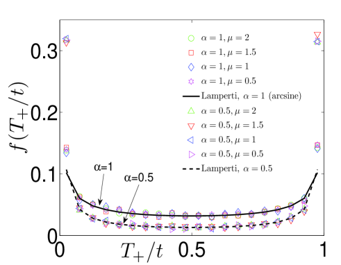
Figure 1: The PDF of the occupation fractions in half-space $T_{+}/t$. Trajectories of diffusing particles were generated using the methods of MagdziarzSimulations1 ; FriedrichSimulations ; MagdziarzSimulations2 with parameter values $\Delta\tau=\overline{\Delta\tau}=10^{-3}$, $\Delta t=10^{-2}$ (as defined in MagdziarzSimulations1 ), $K_{\alpha}=1$, and $x_{0}=0$. Simulations ended at $t=10^{4}$ and included $10^{4}$ trajectories. Simulation results for $\alpha=0.5,1$ and $\mu=0.5,1,1.5,2$ (see Eq. (21)) are shown as symbols (see legend). Theoretical curves correspond to Lamperti’s PDF, Eq. (25) (the arcsine distribution for $\alpha=1$), and are plotted as a solid line for $\alpha=1$ and as a dashed line for $\alpha=0.5$. It can be seen that the distribution of occupation fractions is determined by $\alpha$ but not by $\mu$.

3.2 First passage time

The time $t_{f}$ when a particle starting at $x_{0}=0$ first hits $x=b$ is called the first passage time and is a quantity subject to many studies in physics and other fields Redner_book . The distribution of first passage times for anomalous paths can be obtained from our fractional Feynman-Kac equation using an identity due to Kac Kac1951 :

$$\textrm{Pr}\{t_{f}>t\}=\textrm{Pr}\{\max_{0\leq\tau\leq t}x(\tau)<b\}=\lim_{p\rightarrow\infty}G_{x_{0}}(p,t),$$ (27)

where the functional is $A_{f}=\int_{0}^{t}U[x(\tau)]d\tau$, and

$$U(x)=\begin{cases}0&x<b,\\ 1&x>b.\end{cases}$$ (28)

This is true since $G_{x_{0}}(p,t)=\int_{0}^{\infty}e^{-pA_{f}}G_{x_{0}}(A_{f},t)dA_{f}$, and thus, if the particle has never crossed $x=b$, we have $A_{f}=0$ and $e^{-pA_{f}}=1$, while otherwise, $A_{f}>0$ and for $p\rightarrow\infty$, $e^{-pA_{f}}=0$. To find $G_{x_{0}}(p,t)$ we solve the following backward equation

$$sG_{x_{0}}(p,s)-1=\begin{cases}K_{\alpha}s^{1-\alpha}\frac{\partial^{2}}{\partial x_{0}^{2}}G_{x_{0}}(p,s)&x_{0}<b,\\ K_{\alpha}(s+p)^{1-\alpha}\frac{\partial^{2}}{\partial x_{0}^{2}}G_{x_{0}}(p,s)-pG_{x_{0}}(p,s)&x_{0}>b.\end{cases}$$

Solving these equations as in the previous subsection, demanding that $G_{x_{0}}(p,s)$ is finite for $|x_{0}|\rightarrow\infty$ and demanding continuity of $G_{x_{0}}(p,s)$ and its first derivative at $x_{0}=b$, we obtain for $x_{0}=0$

$$G_{0}(p,s)=\frac{1}{s}\left[1-e^{-\frac{b}{\sqrt{K_{\alpha}}}s^{\alpha/2}}\frac{p(s+p)^{\alpha/2-1}}{s^{\alpha/2}+(s+p)^{\alpha/2}}\right].$$

To find the first passage time distribution we take the limit of infinite $p$,

$$\lim_{p\rightarrow\infty}G_{0}(p,s)=\frac{1}{s}\left(1-e^{-\frac{b}{\sqrt{K_{\alpha}}}s^{\alpha/2}}\right).$$ (29)

Defining $\tau_{f}=(b^{2}/K_{\alpha})^{1/\alpha}$, we invert $s\rightarrow t$:

$$\lim_{p\rightarrow\infty}G_{0}(p,t)=\textrm{Pr}\{t_{f}>t\}=1-\int_{0}^{t}\frac{1}{\tau_{f}}l_{\alpha/2}\left(\frac{\tau}{\tau_{f}}\right)d\tau,$$

where $\l_{\alpha/2}(t)$ is the one-sided Lévy distribution of order $\alpha/2$, whose Laplace transform is $l_{\alpha/2}(s)=e^{-s^{\alpha/2}}$. The PDF of the first passage times, $f(t)$, satisfies $f(t)=\frac{\partial}{\partial t}\left(\textrm{Pr}\{t_{f}<t\}\right)=\frac{\partial}{\partial t}\left(1-\textrm{Pr}\{t_{f}>t\}\right)$. Thus,

$$f(t)=\frac{1}{\tau_{f}}l_{\alpha/2}\left(\frac{t}{\tau_{f}}\right).$$ (30)

This result has been previously derived using different methods (e.g., Eq. (53) of BarkaiPRE01 ). The long times behavior of $f(t)$ is obtained from the $s\rightarrow 0$ limit:

$$f(s)\sim 1-\frac{b}{\sqrt{K_{\alpha}}}s^{\alpha/2}.$$

Therefore, for long times

$$f(t)\sim\frac{b}{|\Gamma(-\frac{\alpha}{2})|\sqrt{K_{\alpha}}}t^{-(1+\alpha/2)}.$$ (31)

For $\alpha=1$, we reproduce the famous $t^{-3/2}$ decay law of a one-dimensional random walk Redner_book .

3.3 The maximal displacement

The maximal displacement of a diffusing particle is a random variable whose study has been of recent interest (see, e.g., Xmax1 ; Xmax2 ; Xmax3 ; Xmax4 and references therein). To obtain the distribution of this variable, we use the functional defined in the previous subsection (Eq. (28)). Let $x_{m}\equiv\displaystyle\max_{0\leq\tau\leq t}x(\tau)$, and recall from Eq. (27) that $\textrm{Pr}\{x_{m}<b\}=\displaystyle\lim_{p\rightarrow\infty}G_{x_{0}}(p,t)$. From the previous subsection we have, for $x_{0}=0$ (Eq. (29))

$$\textrm{Pr}\{x_{m}<b\}=\frac{1}{s}\left(1-e^{-\frac{b}{\sqrt{K_{\alpha}}}s^{\alpha/2}}\right).$$

Hence, the PDF of $x_{m}$ is

$$P(x_{m},s)=\frac{s^{\alpha/2-1}}{\sqrt{K_{\alpha}}}e^{-\frac{x_{m}}{\sqrt{K_{\alpha}}}s^{\alpha/2}}.$$

Inverting $s\rightarrow t$, we obtain

$$P(x_{m},t)=\frac{2}{\alpha\sqrt{K_{\alpha}}}\frac{t}{\left(x_{m}/\sqrt{K_{\alpha}}\right)^{1+2/\alpha}}l_{\alpha/2}\left[\frac{t}{\left(x_{m}/\sqrt{K_{\alpha}}\right)^{2/\alpha}}\right]\quad;\quad x_{m}>0.$$ (32)

This PDF has the same shape as the PDF of $x$ up to a scale factor of 2 BarkaiPRE00 , and it is in agreement with the very recent result of Xmax3 , derived using a renormalization group method.

3.4 The hitting probability

The probability $Q_{L}(x_{0})$ of a particle starting at $0<x_{0}<L$ to hit $L$ before hitting $0$ is called the hitting (or exit) probability. The hitting probability has been investigated long time ago for Brownian particles Redner_book and more recently for some anomalous processes HittingMajumdar . For CTRW, it can be calculated using the following functional:

$$U(x)=\begin{cases}0&0<x<L,\\ \infty&\textrm{Otherwise}.\end{cases}$$ (33)

With Eq. (33), $A=\int_{0}^{t}U[x(\tau)]d\tau=0$ as long as the particle did not leave the interval $[0,L]$ and is otherwise infinite. Therefore, $G(x,p,t)=\int_{0}^{\infty}e^{-pA}G(x,A,t)dA$ represents the probability of the particle to be at $x$ at time $t$ without ever leaving $[0,L]$. This is true for all $p$, since $e^{-pA}$ is either 0 or 1 regardless of $p$. At the boundaries, $G(x=0,p,t)=G(x=L,p,t)=0$. At $(0,L)$, the forward fractional Feynman-Kac equation (Eq. (15)) reads, in $s$ space,

$$sG(x,s)-\delta(x-x_{0})=K_{\alpha}s^{1-\alpha}\frac{\partial^{2}}{\partial x^{2}}G(x,s).$$ (34)

Note that Eq. (34) does not depend on $p$ and is equivalent to the fractional diffusion equation, Eq. (16), with absorbing boundary conditions. The solution of Eq. (34) for $x\neq x_{0}$ is

$$G(x,s)=\begin{cases}C_{0}\sinh\left[\frac{s^{\alpha/2}}{\sqrt{K_{\alpha}}}x\right]&x<x_{0},\\ C_{1}\sinh\left[\frac{s^{\alpha/2}}{\sqrt{K_{\alpha}}}(L-x)\right]&x>x_{0}.\end{cases}$$

Matching the solution at $x=x_{0}$ and demanding $\frac{\partial}{\partial x}G(x=x_{0}^{+},s)-\frac{\partial}{\partial x}G(x=x_{0}^{-},s)=-\frac{1}{K_{\alpha}s^{1-\alpha}}$ (from Eq. (34)), we have, for $x>x_{0}$,

$$G(x,s)=\frac{1}{\sqrt{K_{\alpha}}s^{1-\alpha/2}}\frac{\sinh\left(\frac{s^{\alpha/2}}{\sqrt{K_{\alpha}}}x_{0}\right)}{\sinh\left(\frac{s^{\alpha/2}}{\sqrt{K_{\alpha}}}L\right)}\sinh\left[\frac{s^{\alpha/2}}{\sqrt{K_{\alpha}}}(L-x)\right]\;\;;\;x>x_{0}.$$ (35)

The flux of particles that have never before left $[0,L]$ and that are leaving $[0,L]$ at time $t$ through the right boundary is BarkaiPRL99

$$J(L,t)=-K_{\alpha}{\cal D}_{\textrm{RL},t}^{1-\alpha}\frac{\partial}{\partial x}G(x=L,t),$$

where ${\cal D}_{\textrm{RL},t}^{1-\alpha}$ is the Riemann-Liouville fractional derivative, equal to $s^{1-\alpha}$ in Laplace $t\rightarrow s$ space (see Eq. (16)). The hitting probability is the sum over all times of the flux through $L$ Redner_book :

$$Q_{L}(x_{0})=\int_{0}^{\infty}J(L,t)dt=-K_{\alpha}\left.s^{1-\alpha}\frac{\partial}{\partial x}G(x=L,s)\right|_{s=0}.$$

Using Eq. (35), we have

$$Q_{L}(x_{0})=\frac{x_{0}}{L}.$$ (36)

The hitting probability for anomalous diffusion, $\alpha<1$, is the same as in the Brownian case Redner_book . This is expected, since the hitting probability should not depend on the waiting time PDF $\psi(\tau)$.

Note that a backward equation for $Q_{L}(x_{0})$ can be obtained by the much simpler argument that for unbiased CTRW on a lattice, $Q_{L}(x_{0})=\left[Q_{L}(x_{0}+a)+Q_{L}(x_{0}-a)\right]/2$. In the continuum limit, $a\rightarrow 0$, this gives $\frac{\partial^{2}Q_{L}(x_{0})}{\partial x_{0}^{2}}=0$. With the boundary conditions $Q_{L}(x_{0}=0)=0$ and $Q_{L}(x_{0}=L)=1$, Eq. (36) immediately follows (see Redner_book for a binomial random walk).

3.5 The time in an interval

Consider the time-in-interval functional $T_{i}=\int_{0}^{t}U[x(\tau)]d\tau$, where

$$U(x)=\begin{cases}1&|x|<b,\\ 0&|x|>b.\end{cases}$$ (37)

Namely, $T_{i}$ is the total residence time of the particle in the interval $[-b,b]$. Denote by $G_{x_{0}}(T_{i},t)$ the PDF of $T_{i}$ at time $t$ when the process starts at $x_{0}$, and denote by $G_{x_{0}}(p,s)$ the Laplace transform $T_{i}\rightarrow p$, $t\rightarrow s$ of $G_{x_{0}}(T_{i},t)$. $G_{x_{0}}(p,s)$ satisfies the backward fractional Feynman-Kac equation:

$$sG_{x_{0}}(p,s)-1=\begin{cases}K_{\alpha}\left(s+p\right)^{1-\alpha}\frac{\partial^{2}}{\partial x_{0}^{2}}G_{x_{0}}(p,s)-pG_{x_{0}}(p,s)&|x_{0}|<b,\\ K_{\alpha}s^{1-\alpha}\frac{\partial^{2}}{\partial x_{0}^{2}}G_{x_{0}}(p,s)&|x_{0}|>b.\end{cases}$$ (38)

We solve this equation demanding that the solution is finite for $|x_{0}|\rightarrow\infty$,

$$G_{x_{0}}(p,s)=\begin{cases}C_{1}\cosh\left[x_{0}(s+p)^{\alpha/2}/\sqrt{K_{\alpha}}\right]+\frac{1}{s+p}&|x_{0}|<b,\\ C_{0}\exp\left[-|x_{0}|s^{\alpha/2}/\sqrt{K_{\alpha}}\right]+\frac{1}{s}&|x_{0}|>b.\end{cases}$$ (39)

Demanding continuity of $G_{x_{0}}(p,s)$ and its first derivative at $x_{0}=b$ we solve for $C_{1}$ and then obtain for $x_{0}=0$

$$G_{0}(p,s)=\frac{p+s\left\{\cosh\left[\frac{(s+p)^{\alpha/2}}{\sqrt{K_{\alpha}}}b\right]+\frac{(s+p)^{\alpha/2}}{s^{\alpha/2}}\sinh\left[\frac{(s+p)^{\alpha/2}}{\sqrt{K_{\alpha}}}b\right]\right\}}{s(s+p)\left\{\cosh\left[\frac{(s+p)^{\alpha/2}}{\sqrt{K_{\alpha}}}b\right]+\frac{(s+p)^{\alpha/2}}{s^{\alpha/2}}\sinh\left[\frac{(s+p)^{\alpha/2}}{\sqrt{K_{\alpha}}}b\right]\right\}}.$$ (40)

In principle, the PDF $G_{0}(T_{i},t)$ can be obtained from (40) by inverse Laplace transforming $p\rightarrow T_{i}$ and $s\rightarrow t$. However, we could invert Eq. (40) only for $\alpha\rightarrow 0$:

$$G_{0}(T_{i},t)_{\alpha\rightarrow 0}=(1-e^{-b/\sqrt{K_{0}}})\delta(T_{i}-t)+e^{-b/\sqrt{K_{0}}}\delta(T_{i}).$$ (41)

This can be intuitively explained as follows. For $\alpha\rightarrow 0$, the PDF of $x$ becomes time-independent and approaches $G(x,t)\approx\exp(-|x|/\sqrt{K_{0}})/(2\sqrt{K_{0}})$ (Eq. (A1) in BarkaiPRE00 ). With probability $\int_{-b}^{b}G(x,t)dx=1-e^{-b/\sqrt{K_{0}}}$, the particle never leaves the region $[-b,b]$ and thus $T_{i}=t$; with probability $e^{-b/\sqrt{K_{0}}}$, the particle is almost never at $[-b,b]$ and thus $T_{i}=0$.

The first two moments of $T_{i}$ can be obtained from Eq. (40) by

$$\left\langle T_{i}\right\rangle(s)=\left.-\frac{\partial}{\partial p}G_{0}(p,s)\right|_{p=0}\quad;\quad\left\langle T_{i}^{2}\right\rangle(s)=\left.\frac{\partial^{2}}{\partial p^{2}}G_{0}(p,s)\right|_{p=0}.$$

Calculating the derivatives, substituting $p=0$, and inverting, we obtain, in the long times limit,

$$\left\langle T_{i}\right\rangle \sim t^{1-\alpha/2}\frac{b}{\sqrt{K_{\alpha}}\Gamma(2-\alpha/2)},$$

$$\left\langle T_{i}^{2}\right\rangle \sim t^{2-\alpha/2}\frac{2b(1-\alpha)}{\sqrt{K_{\alpha}}\Gamma(3-\alpha/2)}+t^{2-\alpha}\frac{b^{2}(3\alpha-1)}{K_{\alpha}\Gamma(3-\alpha)}.$$ (42)

We verified that Eq. (3.5) agrees with simulations (Fig. 2). The average time at $[-b,b]$ scales as $t^{1-\alpha/2}$ since this is the product of the average number of returns to the interval $[-b,b]$ ($\sim t^{\alpha/2}$) and the average time spent at $[-b,b]$ on each visit ($\sim t^{1-\alpha}$; see Eq. (61) in BarkaiJSP06 ). We also see that for $\alpha<1$, the PDF of $T_{i}$ cannot have a scaling form since $\left\langle T_{i}^{2}\right\rangle\sim t^{2-\alpha/2}\nsim\left\langle T_{i}\right\rangle^{2}\sim t^{2-\alpha}$. For $\alpha=1$, $\left\langle T_{i}\right\rangle\sim t^{1/2}$ and $\left\langle T_{i}^{2}\right\rangle\sim t$.

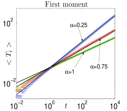
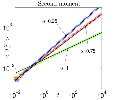
Figure 2: The first two moments of the time-in-interval functional $T_{i}$. Top panel- first moment; bottom panel- second moment. Simulations (circles) were performed using the method of MagdziarzSimulations1 ; FriedrichSimulations with parameters as in Fig. 1. The theoretical curves (lines) correspond to the leading terms of Eq. (3.5). The width of the interval (Eq. (37)) is $b=0.1$.

3.6 Survival in a medium with an absorbing interval

A problem related to that of the previous subsection is a medium in which a diffusing particle is absorbed at rate $R$ whenever it is in the interval $[-b,b]$. The survival probability of the particle, $S$, is related to $T_{i}$, the total time at $[-b,b]$, through $S=\exp(-RT_{i})$. Thus, if $G_{x_{0}}(T_{i},t)$ is the PDF of $T_{i}$ at time $t$, then the $T_{i}\rightarrow R$ Laplace transform $G_{x_{0}}(R,t)=\int_{0}^{\infty}e^{-RT_{i}}G_{x_{0}}(T_{i},t)dT_{i}$ equals $\left\langle S\right\rangle$, the survival probability averaged over all trajectories GrebenkovPRE . From Eq. (40) of the previous subsection we immediately obtain (in Laplace $t\rightarrow s$ space and for $x_{0}=0$)

$$\left\langle S\right\rangle=G_{0}(R,s)=\frac{R+s\left\{\cosh\left[\frac{(s+R)^{\alpha/2}}{\sqrt{K_{\alpha}}}b\right]+\frac{(s+R)^{\alpha/2}}{s^{\alpha/2}}\sinh\left[\frac{(s+R)^{\alpha/2}}{\sqrt{K_{\alpha}}}b\right]\right\}}{s(s+R)\left\{\cosh\left[\frac{(s+R)^{\alpha/2}}{\sqrt{K_{\alpha}}}b\right]+\frac{(s+R)^{\alpha/2}}{s^{\alpha/2}}\sinh\left[\frac{(s+R)^{\alpha/2}}{\sqrt{K_{\alpha}}}b\right]\right\}},$$ (43)

where here $R$ is a parameter (the absorption rate) and thus the equation needs to be inverted only with respect to $s$. We could invert (43) for a few limiting cases.

(i) $t\rightarrow\infty$. The long time behavior is obtained by taking the $s\rightarrow 0$ limit and inverting:

$$\left\langle S\right\rangle\sim\left[\Gamma(1-\alpha/2)\sinh\left(\frac{bR^{\alpha/2}}{\sqrt{K_{\alpha}}}\right)\right]^{-1}(Rt)^{-\alpha/2}+{\cal O}\left[(Rt)^{-\alpha}\right].$$ (44)

Thus, the survival probability of the particle in the absorbing domain decays as $t^{-\alpha/2}$. We verified Eq. (44) using simulations (Fig. 3).

(ii) $\alpha\rightarrow 0$. Inverting Eq. (43) yields

$$\left\langle S\right\rangle_{\alpha\rightarrow 0}=(1-e^{-b/\sqrt{K_{0}}})e^{-Rt}+e^{-b/\sqrt{K_{0}}}.$$ (45)

This can be explained as in the previous subsection. For $\alpha\rightarrow 0$, the PDF of $x$ approaches $G(x,t)\approx\exp(-|x|/\sqrt{K_{0}})/(2\sqrt{K_{0}})$. With probability $\left(1-e^{-b/\sqrt{K_{0}}}\right)$, the particle never leaves the region $[-b,b]$. Thus, its probability of survival is just $e^{-Rt}$. With probability $e^{-b/\sqrt{K_{0}}}$, the particle is almost never in the absorbing zone, and it survives with probability 1.

(iii) Other limiting cases. It can be shown that for $b\rightarrow 0$ or $R\rightarrow 0$, $\left\langle S\right\rangle=1$; for $R\rightarrow\infty$, $\left\langle S\right\rangle=0$; and for $b\rightarrow\infty$, $\left\langle S\right\rangle=e^{-Rt}$.

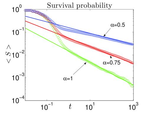
Figure 3: Survival probability in an absorbing medium. We simulated anomalous diffusion trajectories as in Fig. 1 MagdziarzSimulations1 ; FriedrichSimulations , with total time $t=10^{3}$. We plot $\left\langle e^{-RT_{i}}\right\rangle$, where $T_{i}$ is the total time at $[-b,b]$, $R=10$, and $b=1$ (Eq. (37)). Simulation results (symbols) agree with theory (lines), Eq. (44), for $Rt\gg 1$.

3.7 The area under the random walk curve

The functional $A_{x}=\int_{0}^{t}x(\tau)d\tau$ ($U(x)=x$) represents the total area under the random walk curve $x(t)$ FriedrichPLA06 ; NMRReview , and it is also related to the phase accumulated by spins in an NMR experiment NMRReview . In this subsection we obtain the first two moments of this functional, and for a couple of special cases, also its PDF. Since $A_{x}$ is not necessarily positive, we use the generalized forward equation (Eq. (17) Laplace transformed $t\rightarrow s$),

$$sG(x,p,s)-\delta(x)=K_{\alpha}\frac{\partial^{2}}{\partial x^{2}}(s-ipx)^{1-\alpha}G(x,p,s)+ipxG(x,p,s).$$ (46)

Here, $G(x,p,s)$ is the Fourier-Laplace transform of $G(x,A_{x},t)$ and we assumed $x_{0}=0$. Since the walk is unbiased, $\left\langle A_{x}\right\rangle=0$. To find the second moment of $A_{x}$, we use

$$\left\langle A_{x}^{2}\right\rangle(t)=\int_{-\infty}^{\infty}\left.-\frac{\partial^{2}}{\partial p^{2}}G(x,p,t)\right|_{p=0}dx.$$

Integrating Eq. (46) over all $x$, taking the derivatives with respect to $p$ and substituting $p=0$, we obtain

$$s\left\langle A_{x}^{2}\right\rangle(s)=2\left\langle xA_{x}\right\rangle(s),$$ (47)

which is in fact obvious since $\frac{d}{dt}\left(A_{x}\right)=\frac{d}{dt}\left(\int_{0}^{t}x(\tau)d\tau\right)=x$, and thus $\frac{d}{dt}\left\langle A_{x}^{2}\right\rangle=2\left\langle xA_{x}\right\rangle$. Hence, the problem of finding $\left\langle A_{x}^{2}\right\rangle$ reduces to that of finding $\left\langle xA_{x}\right\rangle$, for which we have $\left\langle xA_{x}\right\rangle=\int_{-\infty}^{\infty}-ix\left.\frac{\partial}{\partial p}G(x,p,t)\right|_{p=0}dx$. This leads to

$$s\left\langle xA_{x}\right\rangle(s)=\left\langle x^{2}\right\rangle(s).$$ (48)

Similarly,

$$s\left\langle x^{2}\right\rangle(s)=2K_{\alpha}s^{-\alpha}.$$ (49)

Combining Eqs. (47), (48), and (49), we find $\left\langle A_{x}^{2}\right\rangle(s)=4K_{\alpha}s^{-(3+\alpha)}$, or, in $t$ space,

$$\left\langle A_{x}^{2}\right\rangle(t)=\frac{4K_{\alpha}}{\Gamma(3+\alpha)}t^{2+\alpha}.$$ (50)

Higher moments of $A_{x}$ can be similarly calculated (see next subsection). The distribution of $A_{x}$ can be obtained for a few limiting cases. For $\alpha=1$, $A_{x}$ is normally distributed (Eq. (61) in FriedrichPLA06 ):

$$G(A_{x},t)_{\alpha=1}=\sqrt{\frac{3}{4\pi K_{1}t^{3}}}\exp\left(-\frac{3A_{x}^{2}}{4K_{1}t^{3}}\right).$$ (51)

For $\alpha\rightarrow 0$, the PDF of $x$ is $G(x,t)\approx\exp(-|x|/\sqrt{K_{0}})/(2\sqrt{K_{0}})$ (BarkaiPRE00 and Section 3.5) and is independent of $t$. In other words, the particle is found at $x(t)$ for most of the time interval $[0,t]$. Hence, $A_{x}(t)\approx tx(t)$ and

$$G(A_{x},t)_{\alpha\rightarrow 0}\approx\frac{1}{2\sqrt{K_{0}}t}\exp\left(-\frac{|A_{x}|}{\sqrt{K_{0}}t}\right).$$ (52)

To confirm Eqs. (51) and (52), we plot in Fig. 4 the PDF of $A_{x}$ for various values of $\alpha$ as obtained from simulation of diffusion trajectories. It can also be seen from Fig. 4 that the PDF of $A_{x}$ obeys a scaling relation, as we show in the next subsection.

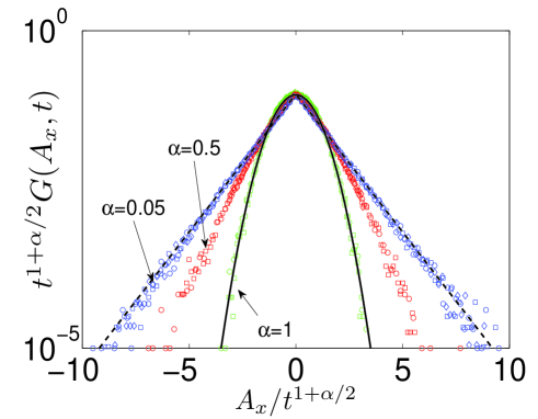
Figure 4: The area under the random walk curve $A_{x}$. We simulated diffusion trajectories as in Fig. 1 MagdziarzSimulations1 ; FriedrichSimulations ($10^{5}$ trajectories) and calculated the PDF $G(A_{x},t)$. To illustrate the scaling, we plot $t^{1+\alpha/2}G(A_{x},t)$ vs. $A_{x}/t^{1+\alpha/2}$ ($K_{\alpha}=1$), collapsing all curves with the same $\alpha$ but different times: $t=1$ (circles), $t=10$ (squares), and $t=100$ (diamonds). Theory for $\alpha=1$ is from Eq. (51) (Gaussian, solid line); theory for $\alpha\rightarrow 0$ is from Eq. (52) (exponential, dashed line).

3.8 The moments of the functionals $U(x)=x^{k}$

In the previous subsection we derived the first two moments of the $U(x)=x$ functional; but in fact, all moments of all functionals $A_{x^{k}}=\int_{0}^{t}x^{k}(\tau)d\tau$, $k=1,2,3,...$ can be obtained, leading to a scaling form of their PDF. As explained above, the functionals with $k=1,2$ arise in the context of NMR and are therefore particularly interesting.

We assume $x_{0}=0$ and consider the forward equation (15) for even $k$’s:

$$sG(x,p,s)-\delta(x)=K_{\alpha}\frac{\partial^{2}}{\partial{x}^{2}}\left(s+px^{k}\right)^{1-\alpha}G(x,p,s)-px^{k}G(x,p,s).$$ (53)

Here, $G(x,p,s)$ is the double Laplace transform of $G(x,A_{x^{k}},t)$ since for even $k$’s $A_{x^{k}}$ is always positive. We are interested in the moments $\left\langle A_{x^{k}}^{n}\right\rangle$, $n=0,1,2,...$; however, to find these, we must first obtain the more general moments $\left\langle A^{n}x^{m}\right\rangle$, $n,m=0,1,2,...$. Operating on each term of Eq. (53) with $(-1)^{n}\frac{\partial^{n}}{\partial p^{n}}$, substituting $p=0$, multiplying each term by $x^{m}$, and integrating over all $x$, Eq. (53) becomes

$$s\left\langle A^{n}x^{m}\right\rangle(s)=\delta_{n,0}\delta_{m,0}+H_{n-1}n\left\langle A^{n-1}x^{m+k}\right\rangle(s)+$$

$$H_{m-2}K_{\alpha}m(m-1)\sum_{j=0}^{n}\binom{n}{j}\left[\prod_{l=0}^{j-1}(1-\alpha-l)\right](-1)^{j}s^{1-\alpha-j}\times$$

$$\times\left\langle A^{n-j}x^{m+jk-2}\right\rangle(s),$$ (54)

where $\delta_{i,j}$ is Kronecker’s delta function— $\delta_{i,j}$ equals 1 for $i=j$ and equals zero otherwise; and $H_{i}$ is the discrete Heaviside function— $H_{i}$ equals 1 for $i\geq 0$ and equals zero otherwise. It can be proved that Eq. (3.8) remains true also for odd $k$’s, when $A_{x^{k}}$ can be either positive or negative. Eq. (3.8) is satisfied by the following choice of $\left\langle A^{n}x^{m}\right\rangle$:

$$\left\langle A^{n}x^{m}\right\rangle(s)=c_{n,m}(k)K_{\alpha}^{\frac{m+nk}{2}}s^{-\left(1+n+\frac{m+nk}{2}\alpha\right)},$$ (55)

for all $n$ and even $m$ when $k$ is even and for even $(n+m)$ when $k$ is odd. In all other cases $\left\langle A^{n}x^{m}\right\rangle=0$ due to symmetry. The $c_{n,m}$’s are $k$-dependent dimensionless constants that satisfy the following recursion equation:

$$c_{n,m}(k)=\delta_{n,0}\delta_{m,0}+H_{n-1}nc_{n-1,m+k}(k)+$$

$$H_{m-2}m(m-1)\sum_{j=0}^{n}\binom{n}{j}\left[\prod_{l=0}^{j-1}(1-\alpha-l)\right](-1)^{j}c_{n-j,m+jk-2}(k),$$ (56)

with initial conditions $c_{0,0}(k)=1$ and $c_{0,1}(k)=0$. The moments of $A_{x^{k}}$ are therefore given in $t$ space by

$$\left\langle A_{x^{k}}^{n}\right\rangle(t)=c_{n,0}(k)\frac{K_{\alpha}^{\frac{nk}{2}}}{\Gamma\left(1+n+\frac{n\alpha k}{2}\right)}t^{n\left(1+\frac{\alpha k}{2}\right)}.$$ (57)

For example, for $k=1$, $\left\langle A_{x}\right\rangle=\left\langle A_{x}^{3}\right\rangle=0$, $\left\langle A_{x}^{2}\right\rangle=4K_{\alpha}t^{2+\alpha}/\Gamma(3+\alpha)$ (Eq. (50)), and $\left\langle A_{x}^{4}\right\rangle=48(\alpha^{2}+7\alpha+12)K_{\alpha}^{2}t^{4+2\alpha}/\Gamma(5+2\alpha)$; while for $k=2$, $\left\langle A_{x^{2}}\right\rangle=2K_{\alpha}t^{1+\alpha}/\Gamma(2+\alpha)$ and $\left\langle A_{x^{2}}^{2}\right\rangle=(48+8\alpha)K_{\alpha}^{2}t^{2+2\alpha}/\Gamma(3+2\alpha)$.

Eq. (57) suggests that the PDF of $A_{x^{k}}$ obeys the scaling relation

$$G(A_{x^{k}},t)=\frac{1}{K_{\alpha}^{k/2}t^{1+\alpha k/2}}g_{\alpha,k}\left(\frac{A_{x^{k}}}{K_{\alpha}^{k/2}t^{1+\alpha k/2}}\right),$$ (58)

where $g_{\alpha,k}(x)$ is a dimensionless scaling function. To verify the scaling form of Eq. (58), we plot in Fig. 4 simulation results for the PDF of $A_{x}$ ($k=1$) for $\alpha\approx 0$ and $\alpha=1$ (for which $G(A_{x},t)$ is known— Eqs. (51) and (52) in the previous subsection), and for an intermediate value, $\alpha=0.5$. In all cases the simulated PDF satisfies the scaling form (58).

4 Summary and discussion

Functionals of the path of a Brownian particle have been investigated in numerous studies since the development of the Feynman-Kac equation in 1949. However, an analog equation for functionals of non-Brownian particles has been missing. Here, we developed such an equation based on the CTRW model with broadly distributed waiting times. We derived forward and backward equations (Eqs. (12) and (20)) and generalizations to Lévy flights (Eqs. (18) and (21)). Using the backward equation, we derived the PDFs of the occupation time in half-space, the first passage time, and the maximal displacement, and calculated the average survival probability in an absorbing medium. Using the forward equation, we calculated the hitting probability and all the moments of $U(x)=x^{k}$ functionals.

The fractional Feynman-Kac equation (12) can be obtained from the integer equation (1) by insertion of a substantial fractional derivative operator FriedrichPRL06 . In that sense, our work is a natural generalization of that of Kac’s. The distributions we obtained for specific functionals are also the expected extensions of their Brownian counterparts: the arcsine law for the occupation time in half-space MajumdarReview ; Watanabe was replaced by Lamperti’s PDF (Eq. (25)) Lamperti , and the famous $t^{-3/2}$ decay of the one-dimensional first passage time PDF Redner_book became $t^{-(1+\alpha/2)}$ (Eq. (31)). Thus, our analysis supports the notion that CTRW and the emerging fractional paths MagdziarzSimulations1 ; FriedrichSimulations are elegant generalizations of ordinary Brownian motion. Nevertheless, other non-Brownian processes are also important. For example, it would be interesting to find an equation for the PDF of anomalous functionals when the underlying process is fractional Brownian motion Mandelbrot .

Our fractional Feynman-Kac equation (12) has the form of a fractional Schrödinger equation in imaginary time. Real time, fractional Schrödinger equations for the wave function have also been recently proposed HuKallianpur ; Laskin2000PRE ; Laskin2002 ; Naber ; SpaceTimeFSE . However, these are very different from our fractional Feynman-Kac equation. In HuKallianpur ; Laskin2000PRE ; Laskin2002 , the Laplacian was replaced with a fractional spatial derivative which would correspond to a Markovian CTRW with heavy tailed distribution of jump lengths (Lévy flights; see also the Appendix below). The approach in Naber ; SpaceTimeFSE is based on a temporal fractional Riemann-Liouville derivative— however not substantial— which leads to non-Hermitian evolution and hence non-normalizable quantum mechanics. It is unclear yet whether all these fractional Schrödinger equations actually describe any physical phenomenon (see Iomin for discussion). In principle, a fractional Schrödinger equation can also be written using the substantial fractional derivative we used here. If there is a physical process behind such a quantum mechanical analog of our equation remains at this stage unclear.

In this paper we considered only the case of a free particle. In BarkaiPRL09 , we reported a fractional Feynman-Kac equation for a particle under the influence of a binding force, where anomalous diffusion can lead to weak ergodicity breaking BarkaiPRL07 ; BarkaiPRL05 ; BarkaiJSP08 . The derivation of an equation for the distribution of general functionals and the treatment of specific functionals for bounded particles will be published elsewhere.

Appendix: Generalization to arbitrary functionals and Lévy flights

Here we generalize our forward and backward fractional Feynman-Kac equations ((12) and (20), respectively) to the case when the functional is not necessarily positive and to the case when the CTRW jump length distribution is arbitrary, and in particular, heavy tailed.

In our generalized CTRW model, the particle moves, after waiting at $x$, to $x+\Delta_{x}$, where $\Delta_{x}$ is distributed according to $f(\Delta_{x})$. The PDF $f(\Delta_{x})$ must be symmetric: $f(\Delta_{x})=f(-\Delta_{x})$ but can be otherwise arbitrary. Let us rederive the forward equation for this model. We replace Eq. (4) with

$$Q_{n+1}(x,A,t)= \int_{0}^{t}\psi(\tau)\int_{-\infty}^{\infty}f(\Delta_{x})Q_{n}[x-\Delta_{x},A-\tau U(x-\Delta_{x}),t-\tau]d\Delta_{x}d\tau.$$

Since $A$ can be negative, we Fourier transform the last equation $A\rightarrow p$

$$Q_{n+1}(x,p,t)=\int_{0}^{t}\psi(\tau)\int_{-\infty}^{\infty}f(\Delta_{x})e^{ip\tau U(x-\Delta_{x})}Q_{n}(x-\Delta_{x},p,t-\tau)d\Delta_{x}d\tau.$$

Laplace transforming $t\rightarrow s$ and Fourier transforming $x\rightarrow k$ we have

$$Q_{n+1}(k,p,s)=\int_{-\infty}^{\infty}e^{ikx}\int_{-\infty}^{\infty}f(\Delta_{x})\hat{\psi}[s-ipU(x-\Delta_{x})]Q_{n}(x-\Delta_{x},p,s)d\Delta_{x}dx.$$

Changing variables: $x^{\prime}=x-\Delta_{x}$,

$$Q_{n+1}(k,p,s) =\int_{-\infty}^{\infty}e^{ik\Delta_{x}}f(\Delta_{x})d\Delta_{x}\int_{-\infty}^{\infty}e^{ikx^{\prime}}\hat{\psi}[s-ipU(x^{\prime})]Q_{n}(x^{\prime},p,s)dx^{\prime}$$

$$=f(k)\hat{\psi}\left[s-ipU\left(-i\frac{\partial}{\partial k}\right)\right]Q_{n}(k,p,s).$$

Summing over all $n$ and using the initial condition $Q_{0}(k,p,s)=e^{ikx_{0}}$,

$$\sum_{n=0}^{\infty}Q_{n}(k,p,s)=\left\{1-f(k)\hat{\psi}\left[s-ipU\left(-i\frac{\partial}{\partial k}\right)\right]\right\}^{-1}e^{ikx_{0}}.$$

Note that this agrees with Eq. (8) since for nearest neighbor hopping $f(k)=\int_{-\infty}^{\infty}e^{ik\Delta_{x}}\left[\frac{1}{2}\delta(\Delta_{x}-a)+\frac{1}{2}\delta(\Delta_{x}+a)\right]d\Delta_{x}=\cos(ka)$. Next, we observe that Eq. (3) of Section 2.1 remains the same even under the general conditions. Calculating the transformed $G(k,p,s)$ as above, and using the result of the last equation, we obtain the formal solution

$$G(k,p,s)= \frac{1-\hat{\psi}\left[s-ipU\left(-i\frac{\partial}{\partial k}\right)\right]}{s-ipU\left(-i\frac{\partial}{\partial k}\right)}\times$$

$$\times\left\{1-f(k)\hat{\psi}\left[s-ipU\left(-i\frac{\partial}{\partial k}\right)\right]\right\}^{-1}e^{ikx_{0}}.$$

We now assume that $f(\Delta_{x})$ has a finite second moment and thus its characteristic function can be written, for small $k$, as $f(k)\sim 1-\sigma^{2}k^{2}/2$. This characteristic function is identical to that of nearest neighbor hopping (with $\sigma=a$); we can thus proceed as in Section 2.1 to obtain

$$\frac{\partial}{\partial t}G(x,p,t)=K_{\alpha}\frac{\partial^{2}}{\partial x^{2}}{\cal D}_{t}^{1-\alpha}G(x,p,t)+ipU(x)G(x,p,t),$$ (59)

where here ${\cal D}_{t}^{1-\alpha}\rightarrow[s-ipU(x)]^{1-\alpha}$ in Laplace $s$ space and $K_{\alpha}=\sigma^{2}/(2B_{\alpha})$.

Consider now the case of Lévy flights— $f(\Delta_{x})\sim|\Delta_{x}|^{-(1+\mu)}$ (for large $\Delta_{x}$) with $0<\mu<2$, and thus jump lengths have a diverging second moment. The characteristic function is $f(k)\sim 1-C_{\mu}|k|^{\mu}$, and the fractional Feynman-Kac equation becomes

$$\frac{\partial}{\partial t}G(x,p,t)=K_{\alpha,\mu}\nabla_{x}^{\mu}{\cal D}_{t}^{1-\alpha}G(x,p,t)+ipU(x)G(x,p,t),$$ (60)

where $K_{\alpha,\mu}=C_{\mu}/B_{\alpha}$ and $\nabla_{x}^{\mu}$ is the Riesz spatial fractional derivative operator: $\nabla_{x}^{\mu}\rightarrow-|k|^{\mu}$ in Fourier $k$ space.

Repeating the calculations of Section 2.2 for a non-necessarily-positive functional and for Lévy flights, it can be shown that the generalized backward equation is:

$$\frac{\partial}{\partial t}G_{x_{0}}(p,t)=K_{\alpha,\mu}{\cal D}_{t}^{1-\alpha}\nabla_{x_{0}}^{\mu}G_{x_{0}}(p,t)+ipU(x_{0})G_{x_{0}}(p,t).$$ (61)

Here, ${\cal D}_{t}^{1-\alpha}\rightarrow[s-ipU(x_{0})]^{1-\alpha}$ in Laplace $s$ space and $\nabla_{x_{0}}^{\mu}\rightarrow-|k_{0}|^{\mu}$ in Fourier $k_{0}$ space.

References

- [1] S. N. Majumdar. Brownian functionals in physics and computer science. Curr. Sci., 89:2076, 2005.
- [2] A. Comtet, J. Desbois, and C. Texier. Functionals of Brownian motion, localization and metric graphs. J. Phys. A: Math. Gen., 38:R341, 2005.
- [3] G. Foltin, K. Oerding, Z. Racz R. L. Workman, and R. P. K. Zia. Width distribution for random-walk interfaces. Phys. Rev. E, 50:R639, 1994.
- [4] G. Hummer and A. Szabo. Free energy reconstruction from nonequilibrium single-molecule pulling experiments. Proc. Natl. Acad. Sci. USA, 98:3658, 2001.
- [5] A. Baule and R. Friedrich. Investigation of a generalized Obukhov model for turbulence. Phys. Lett. A, 350:167, 2006.
- [6] S. N. Majumdar and A. J. Bray. Large-deviation functions for nonlinear functionals of a Gaussian stationary Markov process. Phys. Rev. E, 65:051112, 2002.
- [7] A. Comtet, C. Monthus, and M. Yor. Exponential functionals of Brownian motion and disordered systems. J. Appl. Probab., 35:255, 1998.
- [8] M. Yor. On Exponential Functionals of Brownian Motion and Related Processes. Springer, Germany, 2001.
- [9] M. Kac. On distributions of certain Wiener functionals. Trans. Am. Math. Soc., 65:1, 1949.
- [10] S. Havlin and D. ben-Avraham. Diffusion in disordered media. Adv. Phys., 36:695, 1987.
- [11] J. P. Bouchaud and A. Georges. Anomalous diffusion in disordered media: Statistical mechanisms, models and physical applications. Phys. Rep., 195:127, 1990.
- [12] R. Metzler and J. Klafter. The random walks’s guide to anomalous diffusion: A fractional dynamics approach. Phys. Rep., 339:1, 2000.
- [13] R. Klages, G. Radons, and I. M. Sokolov, editors. Anomalous Transport: Foundations and Applications. Wiley-VCH, Weinheim, 2008.
- [14] B. B. Mandelbrot and J. W. Van Ness. Fractional Brownian motions, fractional noises and applications. SIAM Rev., 10:422, 1968.
- [15] S. N. Majumdar and A. Comtet. Local and occupation time of a particle diffusing in a random medium. Phys. Rev. Lett., 89:060601, 2002.
- [16] E. Barkai. Residence time statistics for normal and fractional diffusion in a force field. J. Stat. Phys., 123:883, 2006.
- [17] A. H. Gandjbakhche and G. H. Weiss. Descriptive parameter for photon trajectories in a turbid medium. Phys. Rev. E, 61:6958, 2000.
- [18] A. Bar-Haim and J. Klafter. On mean residence and first passage times in finite one-dimensional systems. J. Chem. Phys., 109:5187, 1998.
- [19] N. Agmon. Residence times in diffusion processes. J. Chem. Phys., 81:3644, 1984.
- [20] N. Agmon. The residence time equation. Chem. Phys. Lett., 497:184, 2010.
- [21] D. S. Grebenkov. Residence times and other functionals of reflected Brownian motion. Phys. Rev. E, 76:041139, 2007.
- [22] J. Lamperti. An occupation time theorem for a class of stochastic processes. Trans. Am. Math. Soc., 88:380, 1958.
- [23] S. Sabhapandit, S. N. Majumdar, and A. Comtet. Statistical properties of functionals of the paths of a particle diffusing in a one-dimensional random potential. Phys. Rev. E, 73:051102, 2006.
- [24] S. Karlin and H. M. Taylor. A Second Course in Stochastic Processes. Academic Press, New York, 1981.
- [25] D. S. Grebenkov. NMR survey of reflected Brownian motion. Rev. Mod. Phys., 79:1077, 2007.
- [26] E. W. Montroll and G. H. Weiss. Random walks on lattices. II. J. Math. Phys., 6:167, 1965.
- [27] H. Scher and E. Montroll. Anomalous transit-time dispersion in amorphous solids. Phys. Rev. B, 12:2455, 1975.
- [28] R. Friedrich, F. Jenko, A. Baule, and S. Eule. Anomalous diffusion of inertial, weakly damped particles. Phys. Rev. Lett., 96:230601, 2006.
- [29] L. Turgeman, S. Carmi, and E. Barkai. Fractional Feynman-Kac equation for non-Brownian functionals. Phys. Rev. Lett., 103:190201, 2009.
- [30] E. Barkai, R. Metzler, and J. Klafter. From continuous time random walks to the fractional Fokker-Planck equation. Phys. Rev. E, 61:132, 2000.
- [31] M. M. Meerschaert and H. P. Scheffler. Limit theorems for continuous-time random walks with infinite mean waiting times. J. Appl. Prob., 41:623, 2004.
- [32] M. Kotulski. Asymptotic distributions of continuous-time random walks: A probabilistic approach. J. Stat. Phys., 81:777, 1995.
- [33] H. Weissman, G. H. Weiss, and S. Havlin. Transport properties of the continuous-time random walk with a long-tailed waiting-time density. J. Stat. Phys., 57:301, 1989.
- [34] W. R. Schneider and W. Wyss. Fractional diffusion and wave equations. J. Math. Phys., 30:134, 1988.
- [35] H. C. Fogedby. Langevin equations for continuous time Lévy flights. Phys. Rev. E, 50:1657, 1994.
- [36] M. Magdziarz, A. Weron, and K. Weron. Fractional Fokker-Planck dynamics: Stochastic representation and computer simulation. Phys. Rev. E, 75:016708, 2007.
- [37] D. Kleinhans and R. Friedrich. Continuous-time random walks: Simulation of continuous trajectories. Phys. Rev. E, 76:061102, 2007.
- [38] C. Godrèche and J. M. Luck. Statistics of the occupation time of renewal processes. J. Stat. Phys., 104:489, 2001.
- [39] A. Baldassarri, J. P. Bouchaud, I. Dornic, and C. Godrèche. Statistics of persistent events: An exactly soluble model. Phys. Rev. E, 59:20, 1999.
- [40] G. Margolin and E. Barkai. Non-ergodicity of blinking nano crystals and other Lévy walk processes. Phys. Rev. Lett., 94:080601, 2005.
- [41] G. Margolin and E. Barkai. Non-ergodicity of a time series obeying Lévy statistics. J. Stat. Phys., 122:137, 2006.
- [42] F. D. Stefani, J. P. Hoogenboom, and E. Barkai. Beyond quantum jumps: Blinking nano-scale light emitters. Phys. Today, 62:34, 2009.
- [43] S. Watanabe. Generalized arc-sine laws for one-dimensional diffusion processes and random walks. P. Symp. Pure Math., 57:157, 1995.
- [44] M. Kac. On some connections between probability theory and differential and integral equations. In Second Berkeley Symposium on Mathematical Statistics and Probability, page 189, Berkeley, CA, USA, 1951. University of California Press.
- [45] M. Magdziarz and A. Weron. Competition between subdiffusion and Lévy flights: A Monte Carlo approach. Phys. Rev. E, 75:056702, 2007.
- [46] B. Dybiec and E. Gudowska-Nowak. Anomalous diffusion and generalized Sparre Andersen scaling. EPL, 88:10003, 2009.
- [47] S. Redner. A Guide to First-Passage Processes. Cambridge University Press, 2001.
- [48] E. Barkai. Fractional Fokker-Planck equation, solution, and application. Phys. Rev. E, 63:046118, 2001.
- [49] A. Comtet and S. N. Majumdar. Precise asymptotics for a random walker s maximum. J. Stat. Mech., page P06013, 2005.
- [50] S. N. Majumdar, J. Randon-Furling, M. J. Kearney, and M. Yor. On the time to reach maximum for a variety of constrained Brownian motions. J. Phys. A: Math. Theor., 41:365005, 2008.
- [51] G. Schehr and P. Le-Doussal. Extreme value statistics from the real space renormalization group: Brownian motion, Bessel processes and continuous time random walks. J. Stat. Mech., page P01009, 2010.
- [52] V. Tejedor, O. Bénichou, R. Voituriez, R. Jungmann, F. Simmel, C. Selhuber-Unkel, L. B. Oddershede, and R. Metzler. Quantitative analysis of single particle trajectories: mean maximal excursion method. Biophys. J., 98:1364, 2010.
- [53] S. N. Majumdar, A. Rosso, and A. Zoia. Hitting probability for anomalous diffusion processes. Phys. Rev. Lett., 104:020602, 2010.
- [54] R. Metzler, E. Barkai, and J. Klafter. Anomalous diffusion and relaxation close to thermal equilibrium: A fractional Fokker-Planck equation approach. Phys. Rev. Lett., 82:3563, 1999.
- [55] Y. Hu and G. Kallianpur. Schrödinger equations with fractional Laplacians. Appl. Math. Optim., 42:281, 2000.
- [56] N. Laskin. Fractional quantum mechanics. Phys. Rev. E, 62:3135, 2000.
- [57] N. Laskin. Fractional Schrödinger equation. Phys. Rev. E, 66:056108, 2002.
- [58] M. Naber. Time fractional Schrödinger equation. J. Math. Phys., 45:3339, 2004.
- [59] S. Wang and M. Xu. Generalized fractional Schrödinger equation with spacetime fractional derivatives. J. Math. Phys., 48:043502, 2007.
- [60] A. Iomin. Fractional-time quantum dynamics. Phys. Rev. E, 80:022103, 2009.
- [61] A. Rebenshtok and E. Barkai. Distribution of time-averaged observables for weak ergodicity breaking. Phys. Rev. Lett., 99:210601, 2007.
- [62] G. Bel and E. Barkai. Weak ergodicity breaking in the continuous-time random walk. Phys. Rev. Lett., 94:240602, 2005.
- [63] A. Rebenshtok and E. Barkai. Weakly non-ergodic statistical physics. J. Stat. Phys., 133:565, 2008.