Abstract
A common computational problem in multiple change-point models is to recover the segmentations with to change-points of minimal cost with respect to some loss function. Here we present an algorithm to prune the set of candidate change-points which is based on a functional representation of the cost of segmentations. We study the worst case complexity of the algorithm when there is a unidimensional parameter per segment and demonstrate that it is at worst equivalent to the complexity of the segment neighbourhood algorithm: . For a particular loss function we demonstrate that pruning is on average efficient even if there are no change-points in the signal. Finally, we empirically study the performance of the algorithm in the case of the quadratic loss and show that it is faster than the segment neighbourhood algorithm.
A pruned dynamic programming algorithm to recover the best segmentations with to change-points. \titrecourantpDPA to recover the best segmentations with to change-points.
Guillem \nomRigaill\contact[label=e1]rigaill@inra.evry.fr
t1]Institut of Plant Sciences Paris-Saclay (IPS2), UMR 9213/UMR1403, CNRS, INRA, Université Paris-Sud, Université d’Evry, Université Paris-Diderot, Sorbonne Paris-Cité, Bâtiment 630, 91405 0rsay, France
\printcontacte1
Rigaill
multiple-change-point detection \motdynamic programming \motfunctional cost \motsegment neighbourhood
1 Introduction
A common computational problem in multiple change-point models is to recover segmentations with to change-points of minimal cost where the cost is some well chosen criteria, such as minus the log-likelihood or the quadratic loss (Bai and Perron,, 2003; Picard et al.,, 2005; Harchaoui and Cappé,, 2007; Guédon et al.,, 2007; Killick and Eckley,, 2011; Arlot et al.,, 2012; Cleynen and Lebarbier,, 2014; Cleynen et al., 2014a, ). Many algorithms have been proposed to exactly solve this problem (Bellman,, 1961; Fisher,, 1958; Auger and Lawrence,, 1989; Bai and Perron,, 2003; Guédon,, 2008). All these are dynamic programming algorithms and have a complexity which is linear in and quadratic in the length of the signal : . We will refer to these algorithms as segment neighbourhood algorithms.
In practice, this quadratic complexity in is a problem. Indeed, if is larger than or one run of the algorithm can take several hours or even days. In applications such as DNA copy number studies the signal length is typically of this order: -. Several strategies have been developed to cope with this problem, the most famous is probably the binary segmentation heuristic (Scott and Knott,, 1974). A common idea is to first identify a restricted set of candidate change-points with any fast heuristic and then run a segment neighbourhood algorithm on this restricted set (Kolesnikov and Fränti,, 2003; Harchaoui and Lévy-Leduc,, 2010; Gey et al.,, 2008). These heuristics typically have a complexity which is linear in . From a computational perspective the main drawback of these approaches is that they lack optimality.
Most algorithms and heuristics that aim at recovering the segmentations of minimal cost operate on segmentations through their costs. Here we propose a new representation of the segmentations that we call the functional cost where the cost of a segmentation is represented as a function of a, possibly multidimensional, parameter. We demonstrate that using this functional cost it is theoretically possible to prune the set of segmentations while searching for segmentations of minimal costs with to change-points and thus to carry out the calculation only for a small subset of candidate segmentations. We call the resulting algorithm pruned dynamic programming algorithm (pDPA).
From an intuitive point view, if we consider a random sequence of data-points with true abrupt change-points, we expect that the segmentation with those change-points will greatly outperform other possible segmentations in terms of cost. Hence it makes sense that it is possible to efficiently prune the set of segmentations. On the contrary, if we now consider a random sequence of data-points without any change-points, all segmentations will have roughly the same cost and we do not expect an efficient pruning of the set of segmentations. This intuition is indeed true if segmentations are represented through their cost. In the context of another change-point optimization problem, the optimal partitioning problem (Jackson et al.,, 2005), this idea was made particularly clear by Killick et al., (2012).
For this problem, the PELT algorithm, that prunes segmentations based on their cost, was proven to be linear if the true number of change-points is linear in the number of data-points. If it is not linear, in particular if there are no change-points, PELT’s pruning is less efficient.
Here we argue that if we consider the functional costs of segmentations, rather than their costs, we can have an efficient pruning even for random sequences without any change-points. As a proof of concept we study the complexity of the pDPA for change-point models with a unidimensional parameter per segment. In that case, we demonstrate that the algorithm is at worst as efficient as segment neighbourhood algorithms. For a special loss function we demonstrate that on average pruning is efficient even if we consider random sequences without change-points and we retrieve an average complexity which is sub-quadratic in . We implemented the algorithm for the commonly used quadratic loss and empirically show that it is faster than segment neighbourhood algorithms.
Related works
Since the first pre-print of this work (Rigaill,, 2010), the pDPA has been implemented for other losses (Cleynen et al., 2014b, ), and in the context of DNA copy number analysis its competitive runtime compared to the segment neighbourhood algorithm, PELT or other approaches for this problem was confirmed by others (Hocking et al.,, 2013; Hocking,, 2013; Maidstone et al.,, 2014). Furthermore, we demonstrate in this new version of the paper, for a simple, yet non-trivial, loss function that on average the pDPA pruning is efficient even if we consider random sequences without change-points.
Finally, the main contribution of this paper is of a computational nature, i.e an algorithm that recovers the segmentations with to change-points of minimal cost. From a computational point of view several methods boil down to this specific problem. Importantly, the statistical properties of these methods have been studied theoretically and empirically through simulations and on real data by many (Yao and Au,, 1989; Horváth,, 1993; Lavielle and Moulines,, 2000; Lavielle,, 2005; Lebarbier,, 2005; Birgé and Massart,, 2007; Boysen et al.,, 2009; Cleynen and Lebarbier,, 2014; Zhang and Siegmund,, 2007; Lai et al.,, 2005; Cleynen et al., 2014a, ), and recently the pDPA as implemented in the R cghseg package for the quadratic loss was shown to reach state of the art performances for the segmentation of DNA copy number profiles (Hocking et al.,, 2013).
Outline
Section 2 describes the change-point framework used in the paper. Section 3 gives a quick overview of segment neighbourhood algorithms and informally describes the functional cost and the pDPA. Section 4 gives a detailed description of the functional cost and the pDPA. Section 5 is about the worst case, average and empirical complexity of the pDPA.
2 Change-point framework and cost minimization
Data
We assume that we have a sequence of observations. We denote this sequence and denote a subsequence between data-point and data-point , i.e.
Segmentations
We define a segmentation of by a set of change-points splitting the sequence in segments. We denote the positions of these change-points for and we also set the convention that and . We call the -th segment of a segmentation: . is thus the first data-point belonging to and is the first data-point not belonging to . For , we define as the set of all possible segmentations with exactly change-points of the sequence There are such segmentations and so for the whole sequence we have
Statistical model
Our goal is to infer from the data both the positions and the number of change-points. Many methods, statistical models and model selection criteria have been proposed to address this problem for various types of data and various types of changes, i.e. change in the mean, in the variance, in the distribution etc(Lavielle,, 2005; Cleynen and Lebarbier,, 2014; Arlot et al.,, 2012). In practice most of these methods critically rely on algorithms or heuristics that explore the set of all possible segmentations in search for a list of optimal segmentations w.r.t. some well chosen statistical criteria. However, this set of segmentations is extremely large () and it is hard to explore it efficiently, especially when is large.
From a computational point of view this exploration problem is often re-formulated as a cost minimization problem under the constraint that the number of change-points is , where is defined by the user (Bellman,, 1961; Fisher,, 1958; Auger and Lawrence,, 1989; Hawkins,, 2001; Bai and Perron,, 2003; Harchaoui and Cappé,, 2007; Guédon,, 2008; Arlot et al.,, 2012; Cleynen and Lebarbier,, 2014; Guédon,, 2013). To be more specific, the aim is to find the segmentations of minimal cost in for from to , where the cost of a segmentation is the sum of the costs of its segments:
| (1) |
with is the cost of the -th segment of .
A smaller class of problems
In this paper, we consider a smaller class of models and methods for which it is possible to write the cost of a segment as follows:
where is a loss function, depending on the data-point and the (possibly multi-dimensional) parameter , and the function is a regularization penalty. For this class of models we show in the following that it is theoretically possible to prune the set of segmentations and we explain how to implement this pruning if is unidimensional.
The quadratic loss belongs to this class of model: . This framework also includes maximum likelihood inference of identically distributed and independent data-points. Indeed, it suffices to take equal to minus the log-likelihood: . Let us give some examples.
-
1.
We can consider a linear model. To do that we take in , in and within a segment we assume that
In that case minus the log-likelihood is
If the variance is known this simplifies to
-
2.
We can also consider the segmentation in the mean of a -dimensional sequence. Here we take in , in and for all within a segment we assume that
In that case minus the log-likelihood is
If the variance is known this simplifies to
-
3.
We could also consider categorical data. Indeed, we can take , in with and assume that within a segment, are independent and follow a multinomial distribution with In that case minus the log-likelihood is
where is the indicator function.
Many segmentation models do not include a regularization penalty (), however, in some cases it can be of interest to include a regularization penalty such as the ridge penalty. We could take this into account by setting . For simplicity, in the rest of this paper we will only consider the case , however extension to is straightforward.
3 Exact segment neighbourhood algorithm and pruning
In this section, we first describe the main update rule of the standard dynamic programming algorithm - often called the segment neighbourhood algorithm - used to recover the segmentations of minimal cost for to :
| (2) |
Then we present the functional cost representation of a segmentation and informally explain how using this representation it is possible to prune the search space of the segment neighbourhood algorithm. In the last subsection (3.5) we explicitly describe the optimal partitioning problem and the advantages and disadvantages of functional pruning over inequality based pruning (as is done in PELT (Killick et al.,, 2012)).
3.1 The segment neighbourhood algorithm update rule
is segment additive, thus the Bellman optimality principle applies and if a segmentation is optimal any sub-segmentation of this segmentation is also optimal. Mathematically, this can be expressed as the following update rule:
| (3) |
This update rule can be performed with an time complexity. Many algorithms developed for various statistical models implement this particular update rule (Fisher,, 1958; Bellman,, 1961; Auger and Lawrence,, 1989; Bai and Perron,, 2003; Guédon,, 2008). This algorithm was called the segment neighbourhood algorithm by Auger and Lawrence, (1989). To recover we need to apply update rule (3) for every smaller than and for every smaller than . The overall time complexity is thus in . Most of these algorithms have an space complexity. However some, like Guédon, (2008), have an space complexity.
3.2 Functional cost
The segment neighbourhood algorithm and in fact most algorithms and heuristics that aim at recovering the segmentation of minimal cost operate on segmentations through their costs, , which are numbers in . Our pruned DPA algorithm is different and uses a slightly more complex representation that we call the functional cost of a segmentation. We define this function of as:
| (4) |
In words, the functional cost, , is the cost of segmentation if the parameter of ’s last segment is set to , rather than the optimal value . The minimum value of the functional cost is simply the cost: i.e.
The functional cost is a more complex representation of a segmentation than the cost, however, it leads to some great simplifications. Namely the functional cost is point additive, i.e if we consider a segmentation of with change-points and the segmentation of with the same change-points we have:
In the next sub-section (3.3) we explain informally how this functional formulation and the point additiveness makes it theoretically possible to prune the set of segmentations.
3.3 Functional cost and pruning
The pDPA searches for:
| (5) |
for to . This is the functional formulation of equation (2). Like the cost (see update rule (3)), the functional cost is segment additive and a similar update rule applies:
| (6) |
Thanks to the point-additiveness of , it is possible to further simplify this update rule. If we consider a given value of , two last change-points and and a time we get the following implication:
| (7) |
In other words, if for a given and the functional cost of last change-point is less than the functional cost of , then this will still be the case for any time point in the future (i.e. for any ). Hence for the parameter value we can discard as it will never be minimal.
If we consider only one value for , this pruning rule can be formalised as the following update rule:
| (8) |
and this update rule can be performed with an time complexity. We only need to compare the values of and .
3.4 Implementing update rule (8) for all possible
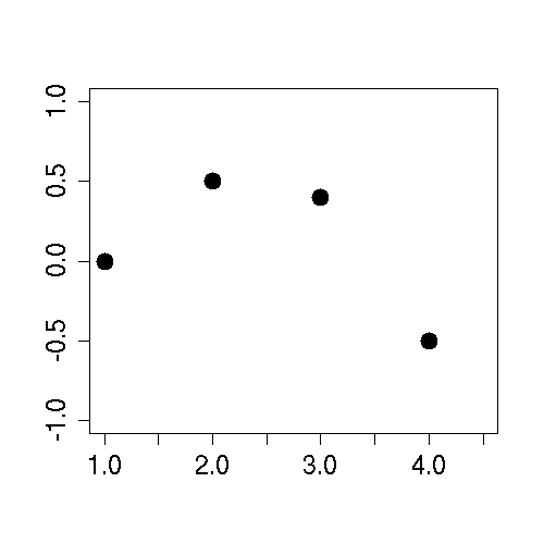
Update rule (8) cannot be implemented in practice, because the rule would have to be applied to all possible values of and in most cases the set of all is uncountably infinite. A key idea to cope with this problem is to consider the set of for which a particular last change-point is better than any other change-point in the sense that is smaller than . We will call this set . We will properly define and study the properties of in section 4. As yet let us have a look at these sets on a small example. We will consider the segmentations with one change-point () of a four-point signal with the quadratic loss: . Our observations are (see Figure 1).
Functional cost of
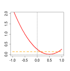
Let us first consider the first two data-points: . The first segmentation we need to consider is the one with a change-point at . The functional cost of this segmentation is simply the cost of its first segment, , which is , plus the functional cost of the last segment, which is the polynomial function . We should also consider a segmentation with a change-point at . Indeed, for its functional cost is well defined: it is the cost of its first segment, , which is , plus the functional cost of its last segment, . is empty and so its functional cost is simply the zero function: . These two functional costs are represented in figure 2-left as a solid red line for and a dashed orange line for . Simple calculations show that the set of for which is best, , is an interval centered on : . is a union of two intervals: . These intervals are also given in figure 2-right.
Functional Cost
| Functional cost | ||
|---|---|---|
| \textcolorred | ||
Functional cost of
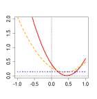
Now if we consider the first three data-points: . We have to update the functional cost of the segmentations having a change-point at and . We do this by adding the function to both of them (point additiveness). We also need to consider another possible change-point: . Its functional cost is simply the cost of segment , which is , plus the function cost of segment which is the zero function: . These three functional costs are represented in figure 3-left as a solid red line for , a dashed orange line for and a blue dotted line for . Simple calculations show that the set of for which is best, , is an interval centered on : . is a union of two intervals: . is strikingly empty. Based on equation (7), this means that irrespective of the last data-point it is sure that the segmentation with a last change-point at will always have a greater cost that those with a change-point at or . Thus for all possible values of we can discard . Note however that neither nor are better than for all .
This simple example illustrates that by keeping track of the we might be able to prune some candidate change-points very early in the process. We will make this idea explicit in the next sections (section 4 and 5).
Functional Cost
| Functional cost | ||
|---|---|---|
| \textcolorred | ||
3.5 Segment Neighbourhood, Optimal partitioning and PELT
Since 2010 another pruned algorithm, PELT, has been proposed for change-point detection problems by Killick et al., (2012). pDPA and PELT are different in nature. First, they do not solve the same problem. PELT is an extension of the optimal partitioning algorithm (Jackson et al.,, 2005) rather than the segment neighbourhood algorithm. More precisely, if we call the set of all segmentations, the optimal partitioning problem is to find:
| (9) |
where is defined in equation (1), is a user defined scalar and is the number of change-points of segmentation . Intuitively, the number of change-points of the recovered solution decreases with . If the penalty is known in advance solving the optimal partitioning problem is faster than solving the segment neighbourhood problem. The advantage of solving the segment neighbourhood problem is that this gives optimal segmentations for a range of numbers of change-points.
Second PELT and the pDPA do not prune segmentations in the same way. PELT’s prune segmentations based on their cost and the pDPA based on their functional cost. In a recent pre-print, Maidstone et al., (2014) called these two ways of pruning respectively inequality based pruning (IP) and functional based pruning (FP) and studied their relationship. The benefit of IP over FP is that it is more widely applicable than FP, i.e. the assumptions on the segment cost to apply FP imply the assumptions to apply IP. Furthermore the implementation of IP is usually straightforward which is not the case of FP. The advantage of FP over IP is that it can prune efficiently the set of change-points even if there are only a few change-points in the sequence. We prove this for a special loss function and under some restrictive conditions in sub-section 5.2. We empirically confirm this result for the quadratic loss in sub-section 5.3. Furthemore, Maidstone et al., (2014) proved in Theorem 6.1 for the optimal partitioning and segment neighbourhood problem that any candidate change-point pruned by IP will also be pruned by FP at worst at the same time. In other words FP cannot prune less than IP.
4 Functional pruning of the set of segmentations
In this section we first describe the key quantities and properties used by the pruned DPA algorithm. Then we describe the algorithm.
4.1 Key quantities and their properties
The four main quantities of interest in the pDPA are given below.
-
1.
the optimal functional cost with change-points:
where the functional cost of a segmentation is defined in equation (4).
- 2.
-
3.
the set of for which the last change-point is optimal:
-
4.
the set of last change-points which are optimal for at least one 111Depending on the properties of it might be possible to consider only the set of last change-points for which is not restricted to a finite set of . This is the case for the quadratic loss which is continuous.
Below are the properties of these quantities. The proofs of these properties are given afterwards.
Property \thetheo
The optimal functional cost may be computed using only the (pruned) set of change-points which are optimal for at least one .
Property \thetheo
The functional cost with a last change-point is easy to update using point additivity.
Property \thetheo
The set of for which a change-point is optimal decreases with (w.r.t. set inclusion) and can be pruned.
| (11) |
| (12) |
| (13) |
Property \thetheo
The set of candidate change-points can be pruned and computed recursively.
Property 4.1 is very similar to the update rule of the segmentation neighbourhood algorithm (equation (3)). The main difference is that the set of last change-points to consider is not necessarily all those before : but rather those that still have a chance to be optimal at this stage: . At worst this is equal to but based on property 4.1 this set could be smaller. Indeed any change-point that has been discarded from will never be included again.
The four previous properties are in fact simple consequences of the point additiveness and segment additiveness of the functional cost. However given their combinatorial nature they might look a bit tedious. To clarify those properties we provide detailed proofs in the following paragraphs.
Proof of property 4.1
As the cost in the segment neighbourhood algorithm, the functional cost of a segmentation is segment additive, thus the Bellman optimality principle holds and we recover the first part of property 4.1. The second part follows by definition of . Indeed, if is the optimal last change-point then there must exist a for which its functional cost is equal to and thus is in
Proof of property 4.1
By definition of (see equation (10)) we have:
Proof of property 4.1
Using property 4.1 and by definition of we get that for :
Proof of property 4.1
By definition of we have
4.2 The pDPA algorithm
The pruned dynamic programming algorithm uses the four properties described in subsection 4.1 to update the optimal functional cost, the set of optimal last change-points and the set of for which these last change-points are optimal. For every and the algorithm:
-
1.
updates for each in the set of for which they are optimal (equation (11));
-
2.
initialises the set of values for which a change-point at is optimal (equation (12));
-
3.
updates the set of possible last change-points (property 4.1);
-
4.
updates the functional cost of possible last change-points (property 4.1);
-
5.
computes the minimal cost with change-points at (property 4.1).
More formally the algorithm can be described as:
Importantly , and are used only at step and . So they need not be stored, they can be discarded or overwritten immediately.
Implementing the pruned DPA
The pruned DPA critically relies on the possibility of easily updating the functional cost () and the set of for which one particular last change-point is optimal (). If this is not the case then the algorithm and the fact that the set of last change-points can be functionally pruned is purely theoretical.
Representing and updating the functional cost is easy typically if there exists a simple analytical decomposition of the functional cost. For example, if we consider the quadratic loss, the functional cost is a second degree polynomial function and it can be represented by the three coefficients of this polynomial function. Other loss functions can be represented in such a way, and in fact the pruned DPA has been implemented for other losses since its first pre-print (namely the Poisson and negative binomial log-likelihood losses, Cleynen et al., 2014b )
Representing the sets is a priori more difficult. Their representation depends on the dimensionality of and the characteristic of the loss function . In the next section we study theoretically and empirically the expected and worst case complexity of functional pruning in the simple case where is a unidimensional parameter in and all functions are unimodals. Here by unimodal we mean functions such that for any in the set is an interval. In that case it is simpler to keep track of the sets and as they are respectively intervals and union of intervals. Functional pruning is theoretically possible even if those conditions are not valid and in particular if is multidimensional. However the implementation and the theoretical study of functional pruning in a multidimensional case is not straightforward and is outside the scope of this paper.
5 Complexity of the algorithm for a unidimensional
In this section we study the complexity of the pruned DPA for in . We also assume that updating the functional cost is in , which is the case if there is a simple analytical decomposition of the functional cost. Finally we will assume that any function is a unimodal function of . This last assumption is true if is convex, which is often the case if we take to be minus the log-likelihood. Under those conditions all are unions of intervals222Indeed, if all are unimodal functions then all are intervals as is a constant in and all are unimodal. Then using property 4.1 we get by induction that all are unions of intervals..
A key question then is how many intervals do we precisely need. In this section, we propose a bound of this number and using it we bound the worst case complexity of the pDPA and show that it is at worst as efficient as the segment neighbourhood algorithm (see subsection 5.1). Then we theoretically study the average complexity of the pDPA algorithm for a particular loss function for a random sequence without change-points (see subsection 5.2). Finally, we empirically study the complexity of the algorithm for the quadratic loss (see subsection 5.3).
5.1 Worst case complexity of the pDPA
In this section we prove that the pDPA is at worst as efficient as the segment neighbourhood algorithm. More precisely we have the following proposition.
Propostion \thetheo
If all are unimodal in and if both minimising and finding the roots of are in , the pDPA is at worst in time and in space.
Proof.
The key quantity to control is the number of intervals needed to represent . For a given and at step the number of candidate last change-points is obviously bounded by . If all are unimodal, using theorem A.2 (proved in appendix A) we get that the total number of intervals is bounded by . Thus at each step there is at most last change-points and intervals to update. By summing all these bounds from to and for every possible we retrieve an worst case time complexity.
As for the worst case space complexity, we need to store two matrices ( and ) and at each step there is at most candidates and intervals. This gives an space complexity
The previous theorem provides a worst case bound on the complexity. One can wonder in which cases this quadratic complexity in is reached. Let us consider the sequence such that , segmentations with one change-point and the quadratic loss. The best segmentation of has a change-point at . So at step of the pDPA the change-point has not been pruned and in fact all change-points from to haven’t been pruned. Hence, at each step we have at least candidates to update. Hence by summing from to we recover a quadratic complexity: .
5.2 Average pruning of the pDPA with a special loss function and
In this subsection, we prove for a particular loss function and that on average we get an efficient pruning with the functional cost representation even when we consider a random sequence without true change-points. As explained in the introduction this result is not intuitive. In subsection 5.3 we empirically show that this is also the case for the quadratic loss function.
Here, we will use the negative log-likelihood loss of a continuous uniform distribution defined on . This loss function is:
For this particular loss function 333note that any is unimodal. and for , it is possible to bound the average number of candidate last change-points, .
Property \thetheo
For the negative log-likelihood loss, , and for, , independent and identically distributed random variables of density and continuous distribution , and the average time complexity of the pDPA is in .
Proof
The proof of is given in appendix B. We obtain this result by studying the set . More precisely we characterize some simple events for which is empty and compute the probability of these events. Then by taking the expectation and summing over all possible we get the desired result.
For the complexity using theorem A.2 we know that the number of intervals stored by the pruned DPA is always smaller than 2 times the number of candidate change-points. Thus for , for every the pruned DPA updates on average functional costs and intervals. From this the complexity follows
5.3 Empirical complexity of the pDPA
In this section, we empirically assess the efficiency of the pDPA to analyze both simulated and real data in the case of the quadratic loss, . The pDPA was implemented in C++ and was run on a Intel Core i7-3687U3 2.10 GHz. The code is available in the cghseg package on the CRAN at the following webpage (http://cran.r-project.org/web/packages/cghseg/index.html). Here is an example code using this function:
install.packages("cghseg")
library(cghseg)
Kmax <- 40; n <- 10^5;
y <- rnorm(n)
system.time(res_ <- cghseg:::segmeanCO(y, Kmax))
5.3.1 Synthetic data
We simulated a number of sequences with a constant, a sinusoid or a rectangular wave signal. We considered an additional gaussian noise of variance 1, a uniform noise and a Cauchy noise. We also considered the worst case scenario for the pDPA which is, as explained at the end of section 5.1, achieved for We compared the pDPA with the segment neighbourhood algorithm for . For all these tests, we set . We then ran the pDPA alone for larger sequences . The R code to ran the pDPA on these simulations is given in appendix C.
Figures 4-A and B show that for all simulated sequences (coloured dotted and dashed lines) except the worst case scenario (black dashed and crossed line) the pDPA is faster than segment neighbourhood (black solid line). It took roughly 150 seconds for the segment neighbourhood algorithm to process a sequence of data-points. In the worst case scenario the pDPA was able to process data-points in the same amount of time, and for other simulated signals the pDPA was able to process more than million data-points in the same amount of time. The runtime of the pDPA depends on the nature of the noise, for example it is faster for a Cauchy noise (green dotted lines in figure 4-A, B and green box-plots in figure 4-C).
5.3.2 Real data
We download the publicly available project from Gene Expression Omnibus (GEO: http://www.ncbi.nlm.nih.gov/geo/). This data set is made of SNP (Single Nucleotide Polymorphism) array experiments. SNP arrays enable the study of DNA copy number gains and losses along the genome. For this kind of sequence, a multiple change-point model based on the quadratic loss is often used (Picard et al.,, 2005). This model has been shown to reach state of the art performances (Lai et al.,, 2005; Hocking et al.,, 2013).
Each SNP array experiment can be viewed as a sequence of million data-points. We assessed the runtime of the pDPA to process these sequences from data-point to for various values of and again with . The R code is given in appendix D. Runtimes are reported in Figure 4-D. The runtime to process the million data-points was on average 28 seconds and was always smaller than 33 seconds. Note that the runtime performances of the pDPA on such SNP array datasets have been confirmed by Hocking et al., (2013).
| A | 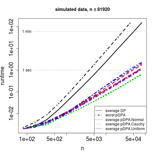 |
B | 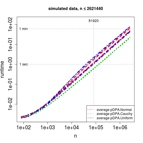 |
| C | 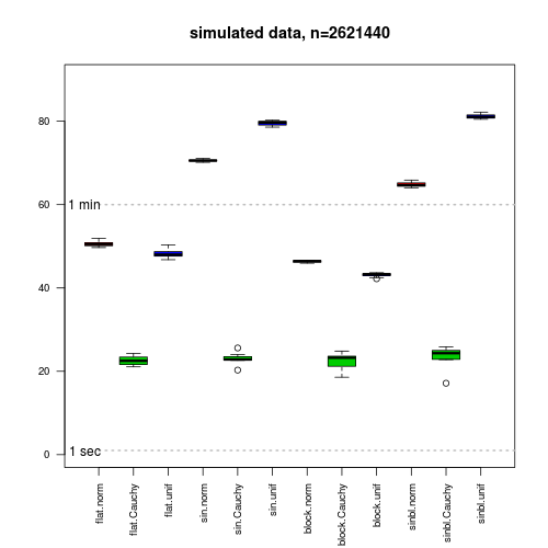 |
D | 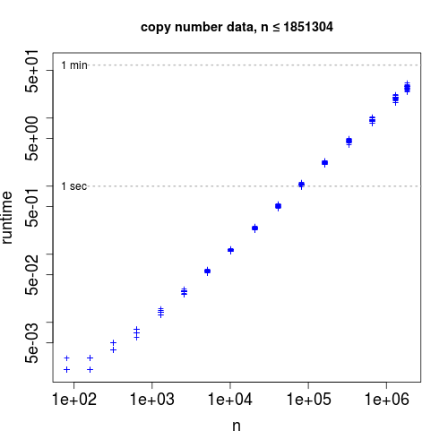 |
Number of intervals
We also directly assess the efficiency of the pruning by counting the number of intervals stored by the pDPA at every time step of the algorithm. Figure 5-A, B and C show, for sequences with a constant or sine wave signal plus an additional gaussian noise and for sequences of the project, the limited number of intervals stored by the pDPA. Indeed, for all these sequences we observed less than 50 intervals. If there was no pruning we would expect at least million and at worst intervals (see subsection 5.1).
| A | 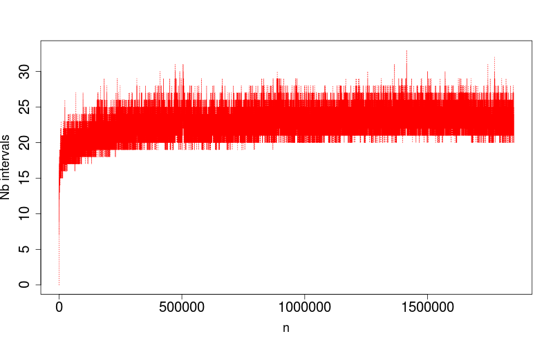 |
B | 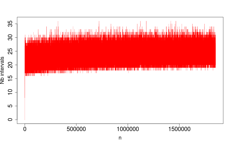 |
|---|---|---|---|
| C | 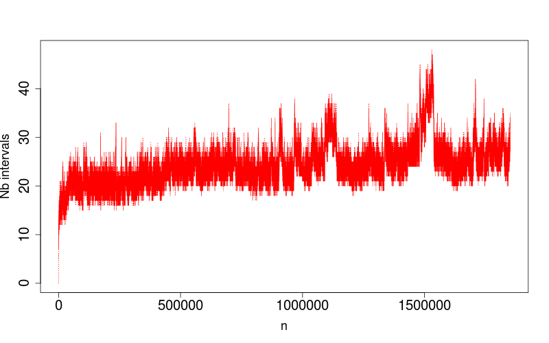 |
6 Conclusion
This paper presented the pDPA that recovers exactly the best segmentations with to change-points of an point sequence w.r.t a loss function. This algorithm is based on a functional representation of the cost of segmentations. For loss functions with a unidimensional parameter per segment the worst case complexity is in , thus the pDPA is at worst equivalent to segment neighbourhood algorithms. For a special loss function it is proven that the pDPA allows to prune the set of candidate change-points efficiently even when there are no change-points in the signal. Finally, in the case of the quadratic loss, it was shown empirically that the pDPA has a small runtime compared to segment neighbourhood algorithms.
Future work
Here we theoretically proved and empirically assessed that functional pruning is efficient under a restrictive set of assumptions. It would be interesting to more generally characterise what are the conditions for functional pruning to be efficient. In particular functional pruning is theoretically possible for a dimensional parameter. Recently, Maidstone et al., (2014) proved that functional pruning prunes at least as much as inequality based pruning. Based on this, it follows that if the conditions of Theorem 3.2 of Killick et al., (2012) are met then functional pruning with optimal partitioning (Fpop) is efficient. However whether functional pruning is on average efficient when is large and the number of change-points is fixed is to our knowledge an open question.
Another question is how to implement functional pruning in the multidimensional case. Indeed this would require an efficient way to represent and update the set of parameter values for which a particular change is optimal. To the best of our knowledge these sets do not have particularly simple properties and are not necessarily easy to handle, except maybe for some special loss functions such as the loss.
Acknowledgement
I would like to thank Alice Cleynen, Michel Koskas, Robert Maidstone, Toby Hocking, Paul Fearnhead, Emilie Lebarbier, Stéphane Robin for fruitful discussions that helped me to better understand the pDPA. Special thanks to Toby, Alban and Patrick.
References
- Arlot et al., (2012) Arlot, S., Celisse, A., and Harchaoui, Z. (2012). Kernel change-point detection. arXiv preprint arXiv:1202.3878.
- Auger and Lawrence, (1989) Auger, I. E. and Lawrence, C. E. (1989). Algorithms for the optimal identification of segment neighborhoods. Bulletin of mathematical biology, 51(1):39–54.
- Bai and Perron, (2003) Bai, J. and Perron, P. (2003). Computation and analysis of multiple structural change models. Journal of Applied Econometrics, 18(1):1–22.
- Bellman, (1961) Bellman, R. (1961). On the approximation of curves by line segments using dynamic programming. Communications of the ACM, 4(6):284.
- Birgé and Massart, (2007) Birgé, L. and Massart, P. (2007). Minimal penalties for Gaussian model selection. Probability theory and related fields, 138(1-2):33–73.
- Boysen et al., (2009) Boysen, L., Kempe, A., Liebscher, V., Munk, A., and Wittich, O. (2009). Consistencies and rates of convergence of jump-penalized least squares estimators. The Annals of Statistics, pages 157–183.
- (7) Cleynen, A., Dudoit, S., and Robin, S. (2014a). Comparing segmentation methods for genome annotation based on rna-seq data. Journal of Agricultural, Biological, and Environmental Statistics, 19(1):101–118.
- (8) Cleynen, A., Koskas, M., Lebarbier, E., Rigaill, G., and Robin, S. (2014b). Segmentor3isback: an r package for the fast and exact segmentation of seq-data. Algorithms for Molecular Biology, 9:6.
- Cleynen and Lebarbier, (2014) Cleynen, A. and Lebarbier, E. (2014). Segmentation of the Poisson and negative binomial rate models: a penalized estimator. ESAIM, P&S, 18:750–769.
- Fisher, (1958) Fisher, W. D. (1958). On grouping for maximum homogeneity. Journal of the American Statistical Association, 53(284):789–798.
- Gey et al., (2008) Gey, S., Lebarbier, E., et al. (2008). Using cart to detect multiple change points in the mean for large sample. SSB preprint.
- Guédon, (2008) Guédon, Y. (2008). Exploring the segmentation space for the assessment of multiple change-point models. hal.inria.fr pre-print inria-00311634.
- Guédon, (2013) Guédon, Y. (2013). Exploring the latent segmentation space for the assessment of multiple change-point models. Computational Statistics, pages 1–38.
- Guédon et al., (2007) Guédon, Y., Caraglio, Y., Heuret, P., Lebarbier, E., and Meredieu, C. (2007). Analyzing growth components in trees. Journal of Theoretical Biology, 248(3):418–447.
- Harchaoui and Cappé, (2007) Harchaoui, Z. and Cappé, O. (2007). Retrospective multiple change-point estimation with kernels. In IEEE Workshop on Statistical Signal Processing.
- Harchaoui and Lévy-Leduc, (2010) Harchaoui, Z. and Lévy-Leduc, C. (2010). Multiple change-point estimation with a total variation penalty. Journal of the American Statistical Association, 105(492).
- Hawkins, (2001) Hawkins, D. M. (2001). Fitting multiple change-point models to data. Computational Statistics & Data Analysis, 37(3):323–341.
- Hocking, (2013) Hocking, T. D. (2013). Comparing least squares segmentation code. available at http://sugiyama-www.cs.titech.ac.jp/ toby/org/HOCKING-ml-seg-compare.pdf.
- Hocking et al., (2013) Hocking, T. D., Schleiermacher, G., Janoueix-Lerosey, I., Boeva, V., Cappo, J., Delattre, O., Bach, F., and Vert, J.-P. (2013). Learning smoothing models of copy number profiles using breakpoint annotations. BMC bioinformatics, 14(1):164.
- Horváth, (1993) Horváth, L. (1993). The maximum likelihood method for testing changes in the parameters of normal observations. The Annals of statistics, pages 671–680.
- Jackson et al., (2005) Jackson, B., Scargle, J. D., Barnes, D., Arabhi, S., Alt, A., Gioumousis, P., Gwin, E., Sangtrakulcharoen, P., Tan, L., and Tsai, T. T. (2005). An algorithm for optimal partitioning of data on an interval. Signal Processing Letters, IEEE, 12(2):105–108.
- Killick and Eckley, (2011) Killick, R. and Eckley, I. A. (2011). Changepoint: an r package for changepoint analysis. R package version 0.6, URL http://CRAN. R-project. org/package= changepoint.
- Killick et al., (2012) Killick, R., Fearnhead, P., and Eckley, I. (2012). Optimal detection of changepoints with a linear computational cost. Journal of the American Statistical Association, 107(500):1590–1598.
- Kolesnikov and Fränti, (2003) Kolesnikov, A. and Fränti, P. (2003). Reduced-search dynamic programming for approximation of polygonal curves. Pattern Recognition Letters, 24(14):2243–2254.
- Lai et al., (2005) Lai, W. R., Johnson, M. D., Kucherlapati, R., and Park, P. J. (2005). Comparative analysis of algorithms for identifying amplifications and deletions in array cgh data. Bioinformatics, 21(19):3763–3770.
- Lavielle, (2005) Lavielle, M. (2005). Using penalized contrasts for the change-point problem. Signal Processing, 85(8):1501–1510.
- Lavielle and Moulines, (2000) Lavielle, M. and Moulines, E. (2000). Least-squares estimation of an unknown number of shifts in a time series. Journal of time series analysis, 21(1):33–59.
- Lebarbier, (2005) Lebarbier, É. (2005). Detecting multiple change-points in the mean of Gaussian process by model selection. Signal processing, 85(4):717–736.
- Maidstone et al., (2014) Maidstone, R., Hocking, T., Rigaill, G., and Fearnhead, P. (2014). On optimal multiple changepoint algorithms for large data. arXiv preprint arXiv:1409.1842.
- Picard et al., (2005) Picard, F., Robin, S., Lavielle, M., Vaisse, C., and Daudin, J.-J. (2005). A statistical approach for array cgh data analysis. BMC bioinformatics, 6(1):27.
- Rigaill, (2010) Rigaill, G. (2010). Pruned dynamic programming for optimal multiple change-point detection. arXiv preprint arXiv:1004.0887.
- Scott and Knott, (1974) Scott, A. and Knott, M. (1974). A cluster analysis method for grouping means in the analysis of variance. Biometrics, 30(3):507–512.
- Yao and Au, (1989) Yao, Y.-C. and Au, S. (1989). Least-squares estimation of a step function. Sankhyā: The Indian Journal of Statistics, Series A, pages 370–381.
- Zhang and Siegmund, (2007) Zhang, N. R. and Siegmund, D. O. (2007). A modified Bayes information criterion with applications to the analysis of comparative genomic hybridization data. Biometrics, 63(1):22–32.
Appendix A Bound on the number of intervals
In this section, we study a special class of functions that we denote and demonstrate theorem A.2. A direct application of this theorem shows that if there are candidate last change-points, then the pDPA need to store at most intervals. We used this theorem in section 4 to prove the worst-case complexity of the pDPA.
A.1 functions
Definition A.1.1
Let denote the set of all functions such that
where all are real numbers and all are
unimodal functions of 444Here by unimodal we mean functions such that for any in the set is an interval. and any is also unimodal . Note that . Let .
If the loss function and any are unimodal in , is part of because we have: .
Definition A.1.2
For any and a subset of we define the function as
Property \thetheo
It is easily shown for with and thus by induction it is true for any .
Definition A.1.3
The rank of a function is
A.2 Decomposition in intervals and order of
Definition A.2.1
Let be a partition of in a finite set of intervals . is a -decomposition of a function if
The set of all functions with a -decomposition is denoted . Similarly the set of all functions with a -decomposition is denoted .
Definition A.2.2
The order of a function is
For all , we have .
Proof
We demonstrate this theorem by induction. It is true if . Assume it is true for any with . Let with . We have:
where :
Let be the smallest set of intervals such that:
Let be the subset of defined as .
As and as for all in is unimodal, there exists a unique such that and therefore . In each interval , we have . By induction, . Overall, for any with , we have:
Appendix B Lower bound on the probability that is empty
Model
We consider the negative log-likelihood loss of a continuous uniform distribution defined on . The loss function is:
| otherwise |
This loss function is unimodal and any sum of is also unimodal. Indeed, for any we have:
| otherwise |
We define We have
Finally note that the loss is continuous to the right and as explained in the footnote page 1 we can further restrict to the set of such that is not restricted to a single value.
Proof
Using equation 12 we get that for any greater than 2 we have:
| (14) | |||||
| (15) |
with There are two cases in which it can be shown that is empty or restricted to a single value and thus can be discarded.
Case 1
: If we have that . Thus we have
and by induction we get .
Case 2
Let us now compute the probability of these two events.
All are independent, they have the same density and continuous distribution , thus the distribution of is and . As is independent of we get that
Using this, we see that case 1 happens with probability:
and case 2 happens with probability:
Furthermore case 1 and case 2 are disjoint events. Thus the probability that the two occur is the sum . Thus the probability that the change-point has not been discarded at step is lower than . So taking the expectation and summing across all smaller than , we recover that the expected number of non discarded candidate change-points is in .
Appendix C R code to assess the runtime of pDPA on simulated data
Here we provide the R code we used to assess the performances of the pDPA. The code of the pDPA is in C++.
First here is a function to simulate different type of signals.
#### simple simulation function
funSimu_ <- function(n, noise="norm", signal="flat"){
Ψ### signal
Ψif(signal == "flat"){
ΨΨx <- numeric(n) Ψ
Ψ}
Ψif(signal == "sin"){## sin
ΨΨx <- 2*sin(1:n/100)Ψ
Ψ}
Ψif(signal == "block"){## 10 blocks
ΨΨnb=5
ΨΨx <- rep(rep(c(0,2), nb), each=n/(2*nb))[1:n]ΨΨ
Ψ}
Ψif(signal == "sinblock"){## 10 blocks + sin
ΨΨnb=5
ΨΨx <- rep(rep(c(0,2), nb), each=n/(2*nb))[1:n]Ψ+ 2*sin(1:n/100)
Ψ}
Ψif(signal == "linear"){
ΨΨx <- 1:nΨ
Ψ}
Ψ
Ψ### noise
Ψif(noise == "none") ### do nothing
Ψif(noise == "norm") x <- x + rnorm(n)
Ψif(noise == "Cauchy") x <- x +rcauchy(n)
Ψif(noise == "unif") x <- x+ runif(n,0, 1) -0.5
Ψreturn(x)
}
Second, here is a simple function to record the runtime of the algorithm.
simpleStat <- function(x){c(mean(x), sd(x), range(x))}
#### simple function to test the runtimes for various n
testRunTime <- function(Kmax = 50, ns=c(100, 200), rep=5,
ΨΨfunSimu=rnorm, noise, signal){
ΨrTime <- list()
Ψfor(n in ns){
Ψcat("Size:", n , ", Repetition 1/", rep, "\n")
Ψfor(j in 1:rep){
Ψx <- funSimu(n, noise=noise, signal=signal)
ΨrTime[[length(rTime)+1]] <- c("pDPA", n, j,
ΨΨsystem.time(res_p <- cghseg:::segmeanCO(x, Kmax=Kmax))[3])
Ψ}
Ψ}
Ψ### formating the runtimes
ΨdTime <- data.frame(matrix(unlist(rTime), ncol=4, byrow=TRUE))
Ψcolnames(dTime) <- c("Algo", "n", "rep", "time")
ΨdTime$time <- as.numeric(as.vector(dTime$time))
ΨdTime$n <- as.numeric(as.vector(dTime$n))
ΨmTime <- aggregate(dTime$time, by=list(dTime$Algo, dTime$n),
ΨΨFUN= simpleStat, simplify=TRUE )
ΨmTime <- cbind(mTime[, 1:2], mTime[, 3][, 1:4])
Ψcolnames(mTime) <- c("Algo", "n", "mean", "sd", "min", "max")
ΨmTime$signal <- signal
ΨmTime$noise <- noise
ΨmTime <- mTime[order(mTime$n), ]
Ψreturn(mTime)Ψ
}
Here is a code to run the algorithm for different types of signal (constant, sinusoid, block), various types of noise (gaussian, uniform and Cauchy) and different values of .
install.packages("cghseg")
require(cghseg)
### 20 000 +
Kmax=40
ns <- 40* 2^(1:16)
respDPA_l <- list()
for(signal in c("flat", "sin", "block", "sinblock")){
print(paste("###", signal))
for(noise in c("norm", "Cauchy", "unif")){
print(noise)
respDPA_l[[length(respDPA_l)+1]] <- testRunTime(Kmax = Kmax, ns=ns, rep=5,
ΨΨfunSimu=funSimu_, noise=noise, signal=signal)
}}
save(respDPA_l, file="respDPA_l.Rdata", compress=TRUE)
Here is a code to run the algorithm in the worst case scenario,
Kmax=40
ns <- 40* 2^(1:10)
respDPA_w <- list()
respDPA_w <- list()
for(signal in c("linear")){
print(paste("###", signal))
for(noise in c("none")){
print(noise)
respDPA_w[[length(respDPA_w)+1]] <- testRunTime(Kmax = Kmax, ns=ns, rep=5,
ΨΨfunSimu=funSimu_, noise=noise, signal=signal)
}}
save(respDPA_w, file="respDPA_w.Rdata", compress=TRUE)
Appendix D R code to assess the runtime of the pDPA on the GSE17359 data set
Here we provide the R code we used to assess the performance of the pDPA on the data from the GSE17359 data set.
dat <- read.table("GSE17359_affy_snp_ratios_matrix.txt", header=TRUE, sep="\t")
require(cghseg)
ie <- which(apply(is.na(dat), 1, sum) == 0)
dat <- dat[ie,]
ns <- c(40* 2^(1:15), nrow(dat))
Kmax = 40
rTime <- list()
for(iSample in 2:ncol(dat)){
print(iSample)
Ψfor(n in ns){
Ψx <- dat[1:n, iSample]
ΨrTime[[length(rTime)+1]] <- c("pDPA", n, iSample,
ΨΨΨsystem.time(res_p <- cghseg:::segmeanCO(x, Kmax=Kmax))[3])
Ψ}
}
dTime <- data.frame(matrix(unlist(rTime), ncol=4, byrow=TRUE))