Maximin design on non hypercube domain and kernel interpolation
Abstract
In the paradigm of computer experiments, the choice of an experimental design is an important issue.
When no information is available about the black-box function to be approximated, an exploratory design has to be used.
In this context, two dispersion criteria are usually considered: the minimax
and the maximin ones. In the case of a hypercube domain, a standard strategy consists
of taking the maximin design within the class of Latin hypercube designs.
However, in a non hypercube context, it does not make sense to use the Latin hypercube strategy.
Moreover, whatever the design is, the black-box function is typically approximated thanks to kernel
interpolation. Here, we first provide a theoretical justification to the maximin criterion with respect to kernel interpolations.
Then, we propose simulated annealing algorithms to determine maximin designs in any bounded connected domain.
We prove the convergence of the different schemes. Finally, the methodology is applied on a challenging real example
where the black-blox function describes the behaviour of an aircraft engine.
Keywords: computer experiments, kernel interpolation, Kriging, maximin designs, simulated annealing.
1 Introduction
A function is said to be an expensive black-box function if is only known through a time consuming code. It is assumed that is enclosed in a known bounded set of . is not necessarily a hypercube domain or explicit. may be given through an indicator function only. It is assumed that testing if a point belongs to is not burdensome. Hence simulate a point in can be performed by sampling rejection. In order to deal with some concerns such as pre-visualization, prediction, optimization and probabilistic analysis which depend on , an approximation of is usually used. This is the paradigm of computer experiments (Santner et al.,, 2003; Fang et al.,, 2005) where the unknown function is deterministic. An approximation of can be obtained using a kernel interpolation method (Schaback,, 1995, 2007). For the corresponding covariance structure, the Best Linear Unbiased Predictor (BLUP) given by Kriging metamodeling (Matheron,, 1963) provides the same approximation of . Due to its flexibility and its adaptivity to non-linear functions, Kriging is one of the most used approximation method by the computer experiments’ community. In our tests, we have observed that Kriging works well for approximating a large class of non linear functions when the input space is of dimension less than ten. For more details on Kriging, one can see for instance: Sacks et al., 1989b ; Sacks et al., 1989a ; Cressie, (1993); Laslett, (1994); Stein, (1999, 2002); Li and Sudjianto, (2005); Joseph, (2006); den Hertog et al., (2006).
The kernel interpolation methodology needs the choice of a kernel (kernel satisfying some conditions detailed below) and a design where the function is to be evaluated, giving . As it is well-known, a space of functions is associated to . If the function belongs to , we can control the pointwise error of , the interpolator of on . In this deterministic paradigm (the function is not random), there are essentially two main kinds of properties that a design can have (Koehler and Owen,, 1996):
- •
-
•
exploratory properties which are warranted by criteria such as:
-
–
minimax which means that the design has to minimize
(1) -
–
maximin which means that the design has to maximize
(2) Moreover, between two designs and such that , using the maximin criterion, we choose the design for which the number of pairs of points with distance equal to is minimal.
-
–
Mean Squared Error (MSE) based criteria. These criteria are linked to the MSE of the BLUP in the context of Kriging metamodeling. Designs can be sought to minimize the Integrated Mean Squared Error (IMSE) of the BLUP over the domain or to minimize the maximum of the MSE over .
-
–
The minimax and maximin criteria have been proposed for Kriging metamodeling by Johnson et al., (1990). Sacks et al., 1989a have detailed the MSE-based criteria. For others criteria, one can see (Bursztyn and Steinberg,, 2006).
For kernels defined by radial basis functions, Schaback, (1995) and Madych and Nelson, (1992) have shown that the mininax criterion explicitly intervenes in an upper bound on the pointwise error between and . The upper bound has the form where is an increasing function . Here, we prove that and then, that a maximin design also provides an uniform upper bound of the pointwise error.
minimax and IMSE criteria are costly to evaluate and, typically, the maximin criterion is privileged. In the case where is a hypercubic set, Morris and Mitchell, (1995) provided an algorithm based on simulated annealing to obtain a design very close to a maximin Latin hypercube designs, (the criterion optimized is not exactly the maximin one). For the two-dimensional case, van Dam et al., (2007) derived explicit constructions for maximin Latin hypercube designs when the distance measure is or . For the distance measure, using a branch-and-bound algorithm, they obtained maximin Latin hypercube designs for .
For some non hypercubic domains, the use of projection properties can lead to poor exploratory designs. For instance, if then, the only Latin hypercube design is on the line . Moreover, in some cases, they are impossible to satisfy. Therefore, we focus on exploratory properties only.
In the case of an explicit constrained subset of , Stinstra et al., (2003) proposed an algorithm based on the use of NLP solvers. Here, we propose some algorithms to achieve a maximin design for general (even not explicit) non hypercubic domains. Our schemes are based on simulated annealing. Our proposals are not heuristic, we study the convergence properties of the schemes proposed.
Recall that the simulated annealing algorithm aims at finding a global extremum of a function by using a Markovian kernel which
is the composition of an exploratory kernel and an acceptance step depending on a temperature which decreases during the iterations.
In some presentations (e.g. Bartoli and Del Moral, (2001)), the simulated annealing algorithm
is based on a Metropolis-Hastings algorithm (Chib and Greenberg,, 1995).
In that case, it can be proved that the resulting Markov chain tends to concentrate
on a global extremum of the function to be optimized with high probability
when the number of iterations tends to infinity.
Here, we introduce a simulated annealing scheme based on a Metropolis-within-Gibbs algorithm
(Roberts and Rosenthal,, 2006) and prove its convergence.
The paper is organized as follows, in Section 2 the kernel interpolation method is described and a theoretical justification of the minimax and maximin criteria is provided thanks to the pointwise error bound between the interpolator and the function . Then, in Section 3 the simulated annealing algorithm is presented. A proof of convergence is given. Section 4 deals with the case where is not explicit and can only be known by an indicator function. Two variants of the algorithm are proposed and their theoretical properties are stated. In Section 5, the algorithms are tried on some examples and practical issues are discussed. Finally, in a last Section, the methodology is applied on a real example for which the domain is not an hypercube.
2 Error bounds with kernel interpolations
A kernel is a symmetric function where is the input space which is assumed to be bounded. The kernel has to be at least conditionally positive definite to be used in kernel interpolation. For the sake of simplicity, kernel interpolation is presented for positive definite kernels only. denotes the space of functions from to .
Definition 2.1.
A kernel is positive definite if
For any , let denote the partial function . The linear combinations of functions taken in span a functional pre-Hilbert space where
is the scalar product. Aronszajn’s theorem states that there exists a unique space which is a completion of where the following reproducing property holds
is called a Reproducing Kernel Hilbert Space (RKHS).
Let us denote by the orthogonal projection of on
( is assumed to be in ; and are given).
Lemma 2.1.
interpolates on . Among the interpolators of on , has the smallest norm: is the solution of the following problem
This interpolator corresponds to the BLUP in the Kriging literature (Cressie,, 1993; Stein,, 2002). It has a Lagrangian formulation.
Lemma 2.2.
For any ,
where the functions are such that, ,
and
where ,
and is such that
.
Hence, the pointwise error can be bounded from above,
Let . depends only on the kernel and
on the design . corresponds to MSE of the BLUP.
When it is integrated on the domain , we obtain the IMSE criterion.
As already explained, the IMSE or the the maximum MSE can be minimized
to determine an exploratory design. However, it depends on the kernel and it is costly to compute.
For some kernels defined by where ,
() and , Schaback, (1995) provides the following upper bound on :
The quantity is associated to the minimax criterion. is an increasing function, obviously depending on the kernel. The smoother the kernel , the faster tends to for . For instance, the Gaussian kernel is defined by where is a real positive parameter; in that case, where and are constants depending on . By choosing a design with a low , one thus ensures a small pointwise error independently of the chosen (radially symmetric) kernel. This justifies using minimax (1) optimal designs. The next proposition shows that a bound on the pointwise interpolation error is still guaranteed when a maximin optimal design is used.
Proposition 2.1.
If is a maximin design, is enclosed in the union of the balls of center and of radius .
Proof
This proposition is proved by contradiction:
let be a maximin design and let us suppose that there exists a point such that
for all .
Let be a pair of points such that and construct
the design where the point is replaced by
the point .
and, in the case ,
is better than with respect to the maximin criterion because the contains less pairs of points
for which the distance is equal to .
Thus, there is a contradiction because is not a maximin design.
Hence, for any , there exists a such that .
As a consequence of this proposition, if is a maximin design,
This result justifies theoretically the use of maximin designs when a kernel interpolation is used as an approximation of . Besides it proves that the interpolation done thanks to a maximin design is consistent since tends to for a sequence of maximin designs of respectively points.
3 Computing maximin designs
In this Section, we propose an algorithm to provide a maximin design with points in any set enclosed in a bounded set. It is based on a simulated annealing method. It aims at finding the global minimum of the function , where is the diameter of the set (). It is obvious that to minimize is equivalent to maximize .
The initialization step consists of simulating uniformly a lot of points in the domain (using sampling rejection) and of calculating the corresponding empirical covariance matrix denoted by . At the end of the initialization step, we randomly keep points, denoted by . An inverse cooling schedule (i.e. is an increasing positive sequence and ) is chosen in order to ensure the convergence of the algorithm. The paramater is a variance parameter which is allowed to change during the iterations but, at each iteration, is such that . A paramater is fixed to be a very small integer to prevent from numerical problems. We propose to iterate the following steps, for :
Algorithm 1.
-
1.
A pair of points is drawn in according to a multinomial distribution with probabilities proportional to ;
-
2.
One of the two points is chosen with probability , it is denoted by ;
-
3.
A constraint Gaussian random walk is used to propose a new point :
is constrained to belong to . The proposed design is denoted by ;
-
4.
with probability
otherwise .
The idea behind this proposal is to force the pairs of points which are very close to be more distant.
In order to explicit the proposal kernel where is an infinitesimal neighborhood of the state , let us introduce some notations:
-
•
,
-
•
,
-
•
denotes the Gaussian pdf with mean and covariance matrix ,
-
•
denotes the normalization constant associated to on the domain .
Let denote the Lebesgue measure on the compact set ( where Leb is the Lebesgue measure on ) and let, for any , denote the Dirac measure with mass at . For a given , let be such that . The proposal kernel reads as, for ,
where for ,
Let us now describe the global kernel associated to Algorithm 1. It obviously depends on the parameters and . It reads as,
where , for .
For and fixed, the algorithm we propose is a random scan Metropolis-within-Gibbs algorithm (Roberts and Rosenthal,, 2006) for which the selection probabilities depend on the current state of the Markov chain. Let denote the Lebesgue measure on the compact set ( where is the Lebesgue measure on ). The target distribution that corresponds to our random scan Metropolis-within-Gibbs is the Gibbs measure defined by
where . In the presentation given by Bartoli and Del Moral, (2001), the simulated annealing algorithm is based on a Metropolis-Hastings algorithm (Hastings,, 1970) and it is assumed that there exists a measure for which the proposal kernel is reversible. In that case, if the target distribution is defined according this measure, the ratio of proposal densities does not appear in the acceptance rate. In our case, there does not exist a reversible measure for , that is why the ratio of the proposal densities is needed.
We will show the convergence of Algorithm 1 following the proof given in Bartoli and Del Moral, (2001). Some Markov chains convergence results are used. Indeed, at a fixed temperature, the Markov chain tends to a stationnary distribution which is the Gibbs measure. As the temperature decreases, the Gibbs measure concentrates on the global extremum of the function. There are typically two properties that are required in the proof: the irreducibility and the invariance of the transition kernel with respect to the Gibbs measure. As already explained, for and fixed, this scheme is a random scan Metropolis-within-Gibbs algorithm with as target. Indeed, using the detailed balance condition, we can easily verified that is -invariant. The irreducibility of this scheme comes from the following result.
Proposition 3.1.
For all non-decreasing sequence and for a sequence such , we have
where and is the smallest positive number such that for all , in , .
Proof
Let us prove first that, for all and , and
, -almost everywhere on .
The fact that is true since the normalization constants are lower-bounded, the Gaussian densities are uniformly
bounded since and all the other terms can be upper bounded by .
The other assertion is only true -almost everywhere on . It means that the lower bound on
holds when and are such that and are both in .
The following lower bounds are used:
-
•
,
-
•
,
-
•
where is the largest eigenvalue of .
is found by multiplying these expressions and, for any , it is a lower bound of which does not depend on and on the states if and have at least points in common.
By definition of , for all and for all -almost everywhere ,
Thus for , .
Then, for all non-decreasing sequence and for a sequence such , we have
is lower bounded with respect to (the Lebesgue measure on the compact set ). We use the following notation
, by definition .
Moreover, for all , we define which is clearly such that
and .
As stated in Bartoli and Del Moral, (2001)
Following the proof of Theorem 4.3.16 in Bartoli and Del Moral, (2001) and using Proposition 3.1, we obtain the convergence of this algorithm.
Theorem 3.1.
If the sequence is such that and if
we get
where denotes the random sequence we get from Algorithm 1 with an initial probability distribution on .
Unfortunately, the function is not regular enough to estimate the convergence speed.
4 Variants of the algorithm
In the case where is not explicit, the normalization constant of a Gaussian distribution with mean and covariance matrix cannot be computed. Hence, the ratio of densities of proposal kernels is not tractable. In that case, we first propose to use as a proposal an unconstrained Gaussian random walk. The steps 3 and 4 of Algorithm 1 are modified.
Algorithm 2.
The first steps until step 3 are the same.
Step 3 is replaced with
-
3bis.
A Gaussian random walk is used to propose a new point :
And step 4 is replaced with
-
4bis.
If , with probability
otherwise .
The proposal kernel corresponding to this algorithm where the Gaussian random walk is not constraint to remain in the domain reads as: for any ,
where for ,
As for Algorithm 1, if is such that and if with , the random sequence we get from Algorithm 2 gives . However, since a point can be proposed outside of the domain , this algorithm can suffer from a lack of efficiency. Another solution is to use the first algorithm without the ratio of densities of proposal kernels.
Algorithm 3.
The first steps until step 4 are the same than in Algorithm 1.
Step 4 is replaced with
-
4ter.
with probability
otherwise .
The global kernel associated to Algorithm 3 is
where . The measure is not -invariant. Hence, we cannot use the Markov chain convergence theory to obtain a result similar to Theorem 3.1. However, is -irreducible and we can easily state the following proposition.
Proposition 4.1.
For all non-decreasing sequence and for a sequence such , we have
where .
As shown in Locatelli, (1996), this proposition leads to the fact that a design reaching a neighborhood of a global maximum of can be achieved in a finite number of iterations almost surely using Algorithm 3.
Proposition 4.2.
For any , if, , with the expected time until the first visit in is finite.
Proof
The expected time until the first visit in is equal to
The aim is to find an upper bound in order to show that it is finite. The second probability in the argument of
the series is limited from above with one. The first probability in the argument of the series is the probability
of never visiting in the first steps.
It can also be written as:
Thanks to Proposition 4.1, it holds that
Thus,
And in a similar way,
Hence, the expected time before the first visit in can be bounded from above by
As if , the previous sum is bounded by
If is chosen such that , the sum becomes
which can be bounded above by
which is a convergent series.
Since the best design ever found during the iterations is saved, the previous proposition provides a theoretical guarantee
for Algorithm 3. Moreover, as a direct consequence, the Markov chain defined by with
is such that .
In practice, is finite and the chosen design is and not . Also, we can consider
that the previous convergence result is sufficient. However, this kind of result can be obtained with any algorithm producing a Markov chain
which well visits the space of states even if the temperature is fixed! Algorithm 3 directly derives from Algorithm 1 and we can expect
that they have similar behaviors.
5 Numerical illustrations
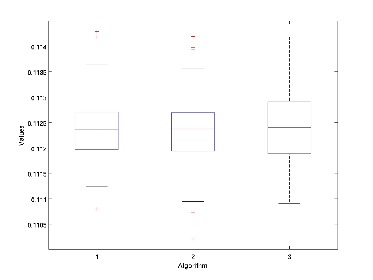
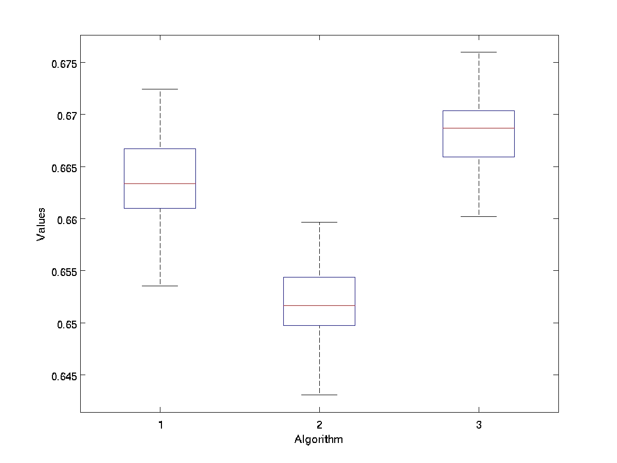
First, the three algorithms are tested on three different toy cases: a design with points in , a design with points in and a design with points in . In these hypercubic cases, the normalization constants can be computed and Algorithm 1 can be used. In each case, calls are made to one million iterations of each algorithm. We observed that the chains produced by the algorithms remain quite stationnary after one million iterations. The inverse cooling schedule is and the variance schedule is .
In order to choose , a lot of designs with points can be drawn uniformly in . Then, a median of , the minimum distance between pair of points in these designs, is computed. Thus, it is a mean to access to an order of magnitude of when is uniformly distributed. A fraction of this value is a good choice for according to our tries. Note that it is much lower than the one required in the convergence theorem.
For , we suggest to use where is the volume of or an upper bound of this volume. Clearly, which parametrizes the random walk variance should not exceed and the previous formula is derived from analogy with a grid. For a -dimensional space, the number of points in a grid reads as where is an integer which corresponds to the number of projected points on each axis. Thus, it seems reasonable to divide the volume of the domain by or more generally by to ensure a good exploration of the space.
Figures 1, 2 and 3 present the results. For each algorithm, the boxplots of the best solutions to the maximization of over one million iterations (boxplots are constructed using 100 replicates) are given. Algorithms 1 and 3 give the best results. Algorithm 2 suffers from the fact that the proposal can be outside of the domain. The computation of is the most time consuming step of these algorithms, that is why the comparison is based on the number of iterations.
Other cooling schedules than the ones which have theoretical guarantees can be tried. It seems that they can lead to satisfying results which are even better than the ones obtained with the schedule. Since the results depend too much on the examples, it is quite hard to state a general rule. However, a schedule is robust to a bad choice in and a schedule performs quite well. The variance decreasing schedule is set to freeze for a given , thus it satisfies the boundedness assumption of the theoretical results.
Finally, in the domain , four strategies are compared to obtain a design with points: taking a design whose points are realizations of a uniform distribution on , taking a lhs-maximin design in with points thanks to the algorithm of Morris and Mitchell, (1995) and keeping the subset which is in only (it gives what we call a truncated lhs-maximin design), using a Sobol’ sequence of points constrained to be in , making use of Algorithm 3. Table 1 displays some statistics on values of for replicates. Only the mean is given for the Sobol’ sequence since it is a deterministic strategy. The truncated lhs-maximin strategy provides designs with approximately points (between and on the replicates).
| Mean | Variance | Min | Max | |
|---|---|---|---|---|
| Uniform | 0.0048 | 0.013 | ||
| Truncated lhs-maximin | 0.034 | 0.025 | 0.039 | |
| Sobol’ sequence | 0.011 | N/A | N/A | N/A |
| Algorithm 3 | 0.080 | 0.079 | 0.081 |
6 Application to a simulator of an aircraft engine
The behavior of an aircraft engine is described by a numerical code. A run of the code determines if the given flight conditions are acceptable and, provided they are, computes the corresponding outputs. The function which associates the outputs to the flight conditions is denoted by . It is accessible only through runs of the code. It is a black box function and a run is time-consuming. A thousand calls to the code are run in ten minutes. The goal is to incorporate the modelization of the engine in a global model of an aircraft for a preliminary design study. Since the simulator of the engine is too burdensome, we are asked to compute an approximation of which can be included in the global model.
The acceptable flight conditions represent the domain of definition of , denoted by . Outside , the code cannot provide outputs since the conditions are physically impossible or the code encounters convergence failures. is not explicit, as explained above we have to run the code to know if the flight conditions are acceptable. Therefore, we need to estimate (the indicator function associated to ). This is not our goal here. is included in a known hypercube (lower and upper bounds are available on each of these variables). Using other prior information and some calls to , a binary classification tree has been built to determine an estimate of the indicator function of (Auffray et al.,, 2011). This method works quite well and leads to a misclassification error rate around . The resulting domain is not an hypercube.
In the following case study, only the flow rate output is focused on. The flight conditions are described by ten variables such as altitude, speed, temperature, humidity… A variable selection procedure has shown that only input variables are useful for prediction (Auffray et al.,, 2011). Hence, the considered function to be approximated is .
A maximin design is drawn thanks to iterations of Algorithm 3. The initial temperature and the initial variance were chosen as described in the previous section. The inverse cooling shedule was and the variance schedule was constant during the first quarter of iterations and then .
Approximations of the function are made by kernel interpolations on four different designs: the maximin design that was computed, a design whose points follow a uniform distribution on , a design obtained by truncating a Latin hypercube design of points defined on the hypercube domain containing and a design given by a low-discrepancy sequence (Sobol) constrained to be in (see Bratley and Fox,, 1988). The lhs is truncated by keeping only the points which belongs to . The kernel interpolations are computed by the Matlab toolbox DACE (Lophaven and Sondergaard,, 2002). The regression functions are chosen as the polynomials with degree smaller than or equal to two and the kernel is a generalized exponential kernel:
where are respectively the coordinates of and are parameters which are estimated using the usual maximum likelihood estimators. Others methods such as cross validation could be used to choose these parameters. The results given in Section 2 only applies when the kernel is isotropic and Gaussian which means and .
The four designs are sets of approximately points which are included in the domain according to the estimated indicator function. For the lhs, we need around points to get approximately points in .
The function is computed at the points of the designs. Some points have to be removed from the designs since the code indicates that they are not in (recall that the designs were built thanks to an estimate of ).
Table 2 provides the performances of kernel interpolations according to the designs. The performances are evaluated on another set of points uniformly distributed in (obtained using sampling rejection) on which the function is also computed. If denotes a kernel interpolator and is the set of test points, those quantities are reported:
-
•
the Mean Relative Error (MRE),
-
•
the Maximum Relative Error (MaxRE),
-
•
the Mean Squared Error (MSE),
Table 2 also contains the number of points which are actually in and the minimal distance between the pairs of points of the designs. To compute these distances, the designs were translated into the hypercube .
| mRE | MaxRE | MSE | Nb of Points | ||
|---|---|---|---|---|---|
| Uniform | 0.49% | 5.2% | 0.63 | 1284 | 0.15 |
| lhs | 0.48% | 6.9% | 0.73 | 1275 | 0.14 |
| maximin | 0.47% | 3.5% | 0.56 | 1249 | 0.33 |
| Sobol’ sequence | 0.46% | 7.7% | 0.62 | 1277 | 0.15 |
The maximin design makes the kernel interpolation more efficient especially according to the MaxRE criterion (although it contains less admissible points than other designs). As it was shown, the kernel interpolation accuracy depends sharply on the spreading out of the points of the design. Thus, the maximin design which ensures that any point of is not far from the points of the design leads to the best performances.
Acknowledgements
The authors are grateful to Pierre Del Moral for very helpful discussions on the convergence properties of the algorithms. This work has been supported by the Agence Nationale de la Recherche (ANR, 212, rue de Bercy 75012 Paris) through the 2009-2012 project Big’MC.

References
- Auffray et al., (2011) Auffray, Y., Barbillon, P., and Marin, J.-M. (2011). Modèles réduits à partir d’expériences numériques. Journal de la Société Française de Statistique, 152(1):89–102.
- Bartoli and Del Moral, (2001) Bartoli, N. and Del Moral, P. (2001). Simulation & algorithmes stochastiques. Cépaduès.
- Bratley and Fox, (1988) Bratley, P. and Fox, B. L. (1988). Algorithm 659: Implementing Sobol’s quasirandom sequence generator. ACM Transactions on Mathematical Software, 14(1):88–100.
- Bursztyn and Steinberg, (2006) Bursztyn, D. and Steinberg, D. M. (2006). Comparison of designs for computer experiments. Journal of Statistical Planning and Inference, 136(3):1103–1119.
- Chib and Greenberg, (1995) Chib, S. and Greenberg, E. (1995). Understanding the Metropolis-Hastings algorithm. The American Statistician, 49(4):327–335.
- Cressie, (1993) Cressie, N. A. C. (1993). Statistics for spatial data. Wiley Series in Probability and Mathematical Statistics: Applied Probability and Statistics. John Wiley & Sons Inc., New York.
- den Hertog et al., (2006) den Hertog, D., Kleijnen, J., and Siem, A. (2006). The correct Kriging variance estimated by bootstrapping. The Journal of the Operational Research Society, 57(4):400–409.
- Fang et al., (2005) Fang, K.-T., Li, R., and Sudjianto, A. (2005). Design and Modeling for Computer Experiments (Computer Science & Data Analysis). Chapman & Hall/CRC.
- Hastings, (1970) Hastings, W. (1970). Monte Carlo Sampling Methods Using Markov Chains and Their Applications. Biometrika, 57(1):97–109.
- Johnson et al., (1990) Johnson, M. E., Moore, L. M., and Ylvisaker, D. (1990). Minimax and maximin distance designs. Journal of Statistical Planning and Inference, 26(2):131–148.
- Joseph, (2006) Joseph, V. R. (2006). Limit kriging. Technometrics, 48(4):458–466.
- Koehler and Owen, (1996) Koehler, J. R. and Owen, A. B. (1996). Computer experiments. In Design and analysis of experiments, volume 13 of Handbook of Statistics, pages 261–308. North-Holland, Amsterdam.
- Laslett, (1994) Laslett, G. M. (1994). Kriging and splines: an empirical comparison of their predictive performance in some applications. Journal of the American Statistical Association, 89(426):391–409.
- Li and Sudjianto, (2005) Li, R. and Sudjianto, A. (2005). Analysis of computer experiments using penalized likelihood in Gaussian Kriging models. Technometrics, 47(2):111–120.
- Locatelli, (1996) Locatelli, M. (1996). Convergence Properties of Simulated Annealing for Continuous Global Optimization. Journal of Applied Probability, 33(4):1127–1140.
- Lophaven and Sondergaard, (2002) Lophaven, N.S., N. H. and Sondergaard, J. (2002). DACE, a Matlab Kriging toolbox. Technical Report IMM-TR-2002-12, DTU.
- Madych and Nelson, (1992) Madych, W. R. and Nelson, S. A. (1992). Bounds on multivariate polynomials and exponential error estimates for multiquadric interpolation. Journal of Approximation Theory, 70(1):94–114.
- Matheron, (1963) Matheron, G. (1963). Principles of Geostatistics. Economic Geology, 58(8):1246–1266.
- McKay et al., (1979) McKay, M., Beckman, R., and Conover, W. (1979). A comparison of three methods for selecting values of input variables in the analysis of output from a computer code. Technometrics, 21(2):239–245.
- Mease and Bingham, (2006) Mease, D. and Bingham, D. (2006). Latin Hyperrectangle Sampling for Computer Experiments. Technometrics, 48(4):467–477.
- Morris and Mitchell, (1995) Morris, M. D. and Mitchell, T. J. (1995). Exploratory designs for computational experiments. Journal of Statistical Planning and Inference, 43:381–402.
- Roberts and Rosenthal, (2006) Roberts, G. O. and Rosenthal, J. S. (2006). Harris recurrence of Metropolis-within-Gibbs and trans-dimensional Markov chains. Annals of Applied Probability, 16(4):2123–2139.
- (23) Sacks, J., Schiller, S., Mitchell, T., and Wynn, H. (1989a). Design and analysis of computer experiments (with discussion). Statistical Science, 4(4):409–435.
- (24) Sacks, J., Schiller, S. B., and Welch, W. J. (1989b). Designs for computer experiments. Technometrics, 31(1):41–47.
- Santner et al., (2003) Santner, T. J., Williams, B. J., and Notz, W. I. (2003). The Design and Analysis of Computer Experiments. Springer Series in Statistics. Springer-Verlag, New York.
- Schaback, (1995) Schaback, R. (1995). Error estimates and condition numbers for radial basis function interpolation. Advances in Computational Mathematics, 3(3):251–264.
- Schaback, (2007) Schaback, R. (2007). Kernel-based meshless methods. Technical report, Institute for Numerical and Applied Mathematics, Georg-August-University Goettingen.
- Stein, (1999) Stein, M. L. (1999). Interpolation of spatial data. Some theory for Kriging. Springer Series in Statistics. Springer-Verlag, New York.
- Stein, (2002) Stein, M. L. (2002). The screening effect in Kriging. The Annals of Statistics, 30(1):298–323.
- Stinstra et al., (2003) Stinstra, E., den Hertog, D., Stehouwer, P., and Vestjens, A. (2003). Constrained maximin designs for computer experiments. Technometrics, 45(4):340–346.
- van Dam et al., (2007) van Dam, E. R., Husslage, B., den Hertog, D., and Melissen, H. (2007). Maximin Latin Hypercube Designs in Two Dimensions. Operations Research, 55(1):158–169.