Graph Approach to Quantum Systems

Abstract

Using a graph approach to quantum systems, we show that descriptions of 3-dim Kochen-Specker (KS) setups as well as descriptions of 3-dim spin systems by means of Greechie diagrams (a kind of lattice) that we find in the literature are wrong. Correct lattices generated by McKay-Megill-Pavicic (MMP) hypergraphs and Hilbert subspace equations are given. To enable future exhaustive generation of 3-dim KS setups by means of our recently found stripping technique, bipartite graph generation is used to provide us with lattices with equal numbers of elements and blocks (orthogonal triples of elements)—up to 41 of them. We obtain several new results on such lattices and hypergraphs, in particular on properties such as superposition and orthoraguesian equations.

I Introduction

We make use of hypergraphs (defined in Sec. III) and bipartite graphs (defined in Sec. V) to describe large 3-dim quantum setups. One way to describe a quantum system in Hilbert space is through the use of lattices, specifically Hilbert lattices (Def. II.3), and our approach is based on a correspondence between graphs and lattices.

Many authors have tried to justify empirically a mathematically well-proved ortho-isomorphism between a Hilbert lattice and the lattice of subspaces of an infinite-dimensional Hilbert space, which has been worked out by over the last 60 years.Beltrametti and Cassinelli (1981); Holland, Jr. (1995) The finite-dimensional case was elaborated even earlier by G. Birkhoff and J. von Neumann.Birkhoff and von Neumann (1936) The results were crowned by the result of Maria Pia SolèrSolèr (1995) that the field (e.g., complex numbers) over which the Hilbert space can be defined follows from the Hilbert lattice conditions.

Yet, a satisfactory empirical justification has not been achieved. First steps have been attempted with a description of spin-1, i.e., 3-dim systems. Several authorsHultgren, III and Shimony (1977); Hultgren, III (1974); Svozil and Tkadlec (1996); Svozil (1998); Tkadlec (1998, 2000, 2001); Smith (2003); Foulis (1999); Pavičić et al. (2004); Pavičić (2009) have obtained a number of results in applications of the so-called Greechie diagrams (see Subsec. II.7) to spin systems. For instance, a correspondence found between orthomodular lattices and MMP hypergraphs (see Sec. III, Def. III.1) enabled an exhaustive generation of all 3-dim Kochen-Specker (KS) sets with up to 24 vectors.Pavičić et al. (2010)

On the other hand, many results on equations holding in Hilbert lattices (see Sec. II.2) have recently been obtained.Megill and Pavičić (2000); Mayet (2006); Pavičić and Megill (2007); Mayet (2007); Megill and Pavičić (2010) An immediate idea was to verify these equations on the sets for which an experimental setups was designed—KS sets. To our surprise it turned out that the standard KS setups described by Greechie diagrams do not allow a verification of these equations. Moreover known KS systems described by Greechie diagrams do not pass even the property of modularity which any spin lattice should pass. Hence, something was missing in the known description of those sets.

A missing link between empirical quantum measurements and its lattice structure was a proper description of a correspondence between the standard quantum measurements, which use Hilbert space vectors and states, and Hilbert lattices, which make use of Hilbert space subspaces that contain these vectors and/or are spanned by them. What hampered a search for such a correspondence was a too narrow focus on orthogonality via lattices represented by Greechie diagrams (Def. II.12).

As we show in Subsec. II.7 Greechie diagrams cannot serve the purpose because they in general turn out not to be subalgebras of a Hilbert lattice (Theorem II.12).

We give two examples which were most elaborated in the literature: empirical reconstruction of quantum mechanics via lattice theory and a description of Kochen-Specker’s setups via lattice theory. The examples show how the application of the Greechie diagrams lead these elaborations to a dead end.

As for the empirical reconstruction, B. O. Hultgren, III and A. Shimony used Greechie diagrams in their detailed attempt to build up a Hilbert lattice of a realistic quantum system for a 3-dim spin-1 system passing through Stern-Gerlach filters.Hultgren, III and Shimony (1977); Hultgren, III (1974) They did not succeed in building a Hilbert lattice because the Greechie diagrams, as we show below (Th. II.12), are not subalgebras of a Hilbert lattice. They failed to obtain some features they thought they should have obtained and they obtained some features they thought they should not have obtained. As for the former features, e.g., superposition, we show that they do not cause necessarily problems (see the remark after Lemma II.2). As for the latter features, it has been shown that their appearance was due to the fact that they did not take into account both electric and magnetic fields.Swift and Wright (1980) However, even if Hultgren and Shimony had used them they could have only repaired some faulty Greechie diagrams. In particular, they could have patched the missing links in their Fig. 3 (dashed lines) and with them their lattice would read: 123,456,789,ABC,58B (using MMP hypergraph encoding, described below).

As for the KS setup, S. Kochen and E. P. SpeckerKochen and Specker (1967) in their proof used a partial Boolean algebra (PBA), which is a very general class of algebras. The closed subspaces of a Hilbert space form a particular, specialised PBA. However, conditions that make PBA isomorphic to a lattice of Hilbert space subspaces have not been discovered, although steps in that direction have been taken by D. Smith.Smith (1999, 2003, 2004) The equivalence of PBA and atomic ortholattices was proved by I. Pitowsky in 1982.Pitowsky (1982) Apparently misled by this equivalence, some authors have represented KS setups by means of Greechie diagrams in a series of publications.Svozil and Tkadlec (1996); Svozil (1998); Tkadlec (1998, 2000, 2001) In Sec. III, we show that KS setups cannot be described by means of Greechie diagrams because Greechie diagrams are not subalgebras of a Hilbert lattice.

Now, in Sec. III we show that both a lattice reconstruction of quantum mechanics and a lattice description of KS setups must take nonorthogonal subsets into account. They are required by the conditions and equations that must hold in every Hilbert space. This is the reason why KS setups cannot be described by means of Greechie diagrams, as we prove for all known spin-1 KS setups, notably Kochen-Specker’sKochen and Specker (1967), Peres’Peres (1991), Kernaghan’sKernaghan (1994), Bub’sBub (1996), and Conway-Kochen’sBub (1996).

We also find a way to obtain lattices that we can use to describe a quantum setup to any desired degree of accuracy. They make use of subspaces that contain non-orthogonal vectors and/or are spanned by them. The subspaces that appear in them are filtered by the aforementioned conditions and equations that must hold in every Hilbert space. We call such lattices MMPLs (see Def. III.2 and Fig. 8).

However, our programs written for a generation of arbitrary MMP hypergraphs that can be used for a construction of MMPLs with more than 30 vectors take too much time. Therefore, we consider lattices that have some of the properties MMPLs require and lack some others, with the idea—which turns out to be rewarding—of getting lattices with more than 40 vectors that can be obtained faster and that can in turn give all interesting MMPLs by means of different very fast algorithms and programs. For instance, to obtain all 4-dim KS sets with 18 through 24 vectors requires several months on a cluster with 500 3GHz CPUs, while in Ref. Pavičić et al., 2010 we found an algorithm and a program to obtain them all from a single KS set with 24 vectors in less than 10 min on a single PC. This 24 vector KS set also belongs to the aforementioned class of lattices that have “some of the properties MMPLs require and lack some others.” Vectors correspond to atoms in lattices and to vertices in MMP hypergraphs, and tetrads correspond to blocks in lattices and edges in MMP hypergraphs. MMP hypergraphs are defined in Ref. Pavičić et al., 2004 and in Sec. III, Def. III.1.

The aforementioned “10 min” method we call a stripping technique.Pavičić et al. (2010) It consists in stripping blocks off of a single initial KS set with 24 vertices (vectors) and 24 edges (tetrads) until we reach the smallest such sets—called critical KS sets—in the sense that any of them would cease to be a KS set if we stripped any further blocks away. The technique provided us with all 1232 KS subsets with vector component values from {-1,0,1} contained in the 24-24 class of KS {-1,0,1} set.

We also applied the same technique to 60-60 KS sets that we obtained from a 60-75 set and generated a huge number of critical sets (for 60-65 through 60-75 we rigorously verified that no critical set exists and for 60-61 through 60-64 we confirmed that statistically with a high confidence). All the KS sets and critical sets we generated in this way form a new KS class (we call it “60-75 KS class”) which is disjoint from the 24-24 class.Pavičić et al. (2010) The smallest critical set from this class is a 13-26 KS set shown in Fig. 1 of Ref. Pavičić et al., 2010.

In the above generation of 4-dim KS sets by the stripping technique we were fortunate to find covering KS sets with the same number of vertices and edges (24-24, 60-60). For 3-dim KS sets no such covering set with the the same number of vertices and edges is known so in this paper we pave the road of its generation by means of bipartite graphs (see Secs. V and VI).

As we report in Sec. V, such a generation of bipartite graphs is still computationally too demanding. We previously considered 3-dim systems with equal number of atoms (vertices) and blocks (edges) with up to 38 atoms and blocks.Pavičić (2009) Now we use much faster algorithms and programs and are able to reach 41 atoms and blocks. This is still not enough for a realistic system, but we obtain several important properties of such classes of lattices that might help us to obtain even better algorithms and reach the 50 atoms required for generation of realistic KS setups with the help of the stripping technique.

The results we invoke and make use of are well-known in lattice theory. They have not been reformulated in Hilbert space theory itself, so, we present all our results in the lattice theory, and only when it would really help the reader to see what a Hilbert-space version of particular properties and axioms would look like, do we formulate some result directly in the Hilbert space parlance as, e.g., in Theorems II.9 and II.10. Hence for the reader who is not too familiar with the lattice theory, we first introduce and characterise its basic notions in Sec. II, and here we give a general framework in which we shall make use of the lattice theory.

A spin state of a system is assumed to be repeatedly prepared, manipulated, and/or filtered by a device. The directions of vectors of the spin projections coincide with the orientations of the device. Hilbert space subspaces that contain these vectors form lattices. To distinguish between device orientations and spin orientations we use the term experimental setup to mean a description of the devices and their fields. We use the term formalised setup to mean a theoretical description of the quantum systems.

We start with a very general class of lattices—orthomodular lattices (OMLs) (see Def. II.2). Elements of spin-1 OMLs correspond to subspaces (1-dim rays and 2-dim planes) spanned by Hilbert space vectors which must satisfy two classes of conditions:

(1) Equations, e.g., the orthoarguesian and Godowski equations (see Table 1 for a summary of these and other equations mentioned);

(2) Quantified expressions, e.g., the superposition principle [Def. II.3(3); Eq. (18)].

They are essential for understanding the ramification of all quantum setups:

(1) Equations that fail in a subalgebra of a lattice will also fail in the lattice (see Lemma II.2 below). So no experimental setup for which quantum mechanical equations cannot have a solution can be used for measuring properties of a quantum system. Such setups are non-quantum setups;

(2) Quantified expressions that fail in a subalgebra of a lattice may, however, pass in the lattice (see the remark after Lemma II.2 below). Smaller setups, in which e.g. superposition cannot be measured, are “sub-setups” of setups in which superposition is possible.

Quantum setups and quantum lattices refer to systems whose OMLs are subalgebras of a Hilbert lattice. Semi-quantum lattices refer to systems whose OMLs are not subalgebras of a Hilbert lattice. Examples of the former are proper KS lattices in the sense of being subalgebras of a Hilbert lattice.

Semi-quantum lattices with equal number of atoms and blocks we consider are atomic lattices. They admit real-valued and vector states, satisfy superposition, and yet violate, e.g., orthoarguesian equations. To deal with them we can use Greechie diagrams because we consider lattices that consist of concatenated orthogonal triples and are not subalgebras of a Hilbert lattice.

To generate semi-quantum lattices we proceed as follows. We first use algorithms that exhaustively generate cubic bipartite graphs. We then show that they are equivalent to MMP hypergraphs which in turn correspond to OMLs with equal numbers of atoms and blocks. We generate OMLs with up to 41 of atoms and blocks, and prove that they all have the above features. The obtained OMLs narrow down the non-quantum classes of OMLs and might enable us to generate quantum classes of OMLs of high complexity and KS setups. They also enable us to obtain several new results in Hilbert lattice theory that rely on the features that the generated OMLs possess. In Sec. V, we analyse the properties of the OMLs obtained in Sec. VI, and provide a new type of graphical representation for them in Sec. VII. We discuss the obtained results in Sec. VIII.

The “negative results” that we consider in this paper (classes of lattices that do not pass particular equations) we have recently used as a tool for generating other equations Megill and Pavičić (2010) and, in the case of the aforementioned 4-dim KS sets, for generating new KS sets.

Our results also provide us with novel algorithms and results in the theory of bipartite graphs and hypergraphs. Lattices that do not admit strong sets of states serve as inputs to algorithms for finding new Hilbert lattice equations, and lattices that admit just one state serve for establishing new lattice features and theorems.Shultz (1974); Navara (2008)

Bipartite graphs have recently been studied extensively in the field of quantum information. A bipartite entanglement of the states constructed from the algebra of a finite group with a bilocal representation ($G$) acting on a separable reference state has been studied in Ref. Hamma et al., 2005. If $G$ is a group of spin flips acting on a set of qubits, these states are locally equivalent to bipartite (two-colorable) graph states and they include GHZ, CSS, cluster states, etc. Equivalence of CSS states (of which GHZ states are a special case) and bipartite graph states has been shown in Ref. Chen and Lo, 2007.

Graph states form class of multipartite entangled states associated with combinatorial graphs (see, e.g., Refs. M.Hein et al., 2004 and Cosentino and Severini, 2009) and have applications in diverse areas of quantum information processing, such as quantum error correction and the one-way model.

On the other hand, bipartite graphs have been shown to have an important application for quantum search and related quantum walks, span-programs, and search algorithms such as Grover’s.Carneiro et al. (2005); Reichardt (2009)

II Preliminary Definitions and Theorems and the Semi-Quantum Lattices

This section covers most definitions and background material. It is organized as follows.

• Hilbert lattices (Subsection II.1)

• Overview of equations holding in Hilbert lattices (Subsection II.2)

• States (Subsection II.3)

• Vector-valued states (Subsection II.4)

• Superposition (Subsection II.5)

• Orthoarguesian equations (Subsection II.6)

• Greechie diagrams (Subsection II.7)

• Semi-quantum lattices (Subsection II.8)

II.1 Hilbert lattices

The closed subspaces of a Hilbert space $\mathcal{H}$ form an algebra called $\mathcal{C}(\mathcal{H})$, which is a member of the class of orthomodular lattices (OML). An OML, in turn, is a member of a more general class called OL (ortholattices). We will first define OLs, OMLs, and related structures, then we will describe how the closed subspaces of Hilbert space form a member of (some) of these classes of structures.

We define OL as follows, along with auxiliary constants $0$ and $1$, an ordering relation, and an implication operation. The binary operations $\cup$ and $\cap$ are called join and meet respectively, and the unary operation ^′ is called orthocomplementation. Recall that an algebra is an $n$-tuple consisting of a base set and $n-1$ operations on that base set.

Definition II.1.

An ortholattice, OL, is an algebra $\langle{\mathcal{OL}}_{0},^{\prime},\cup,\cap\rangle$ such that the following conditions are satisfied for any $a,b,c\in\,{\mathcal{OL}}_{0}$ Megill and Pavičić (2002): $a\cup b\>=\>b\cup a$, $(a\cup b)\cup c\>=\>a\cup(b\cup c)$, $a^{\prime\prime}\>=\>a$, $a\cup(b\cup b\,^{\prime})\>=\>b\cup b\,^{\prime}$, $a\cup(a\cap b)\>=\>a$, and $a\cap b\>=\>(a^{\prime}\cup b\,^{\prime})^{\prime}$. In addition, since $a\cup a^{\prime}=b\cup b\,^{\prime}$ for any $a,b\in\,{\mathcal{OL}}_{0}$, we define the greatest element of the lattice (1) and the least element of the lattice (0), $\textstyle{1}\,{\buildrel\rm def\over{=}}a\cup a^{\prime}$ and  $\rm\textstyle{0}\,{\buildrel\rm def\over{=}}a\cap a^{\prime}$, respectively and the ordering relation ($\leq$) on the lattice: $a\leq b\ \quad{\buildrel\rm def\over{\Longleftrightarrow}}\quad\ a\cap b=a\quad\Longleftrightarrow\quad a\cup b=b$. Quantum (Sasaki) implication is defined as $a\to b=a^{\prime}\cup(a\cap b)$.

When we say a lattice is an OL (or an OML, etc.) we mean that the lattice is a member of the class OL (OML, etc).

By adding an additional condition, we can restrict the class OL to become the successively smaller (less general) classes OML, MOL, and BA as follows.

Definition II.2.

An ortholattice (OL) in which

$$b\leq a\ \&\ c\leq a^{\prime}\ \Rightarrow\ a\cap(b\cup c)=(a\cap b)\cup(a\cap c),$$ (1)

$$b\leq a\ \Rightarrow\ a\cap(b\cup c)=(a\cap b)\cup(a\cap c),$$ (2)

or $$a\cap(b\cup c)=(a\cap b)\cup(a\cap c)$$ (3)

holds, is an orthomodular lattice (OML), modular ortholattice (MOL), or Boolean algebra (BA), respectively.

Our primary interest is in the subclass of OML called HL (Hilbert lattices).

Definition II.3.

An orthomodular lattice that satisfies the following conditions is a Hilbert lattice (HL).

1. Completeness: The meet and join of any subset of an HL exist.

2. Atomicity: Every non-zero element in an HL is greater than or equal to an atom. (An atom $a$ is a non-zero lattice element with $0<b\leq a$ only if $b=a$.)

3. Superposition principle: (The atom $c$ is a superposition of the atoms $a$ and $b$ if $c\neq a$, $c\neq b$, and $c\leq a\cup b$.)

   (a)

   Given two different atoms $a$ and $b$, there is at least one other atom $c$, $c\neq a$ and $c\neq b$, that is a superposition of $a$ and $b$.

   (b)

   If the atom $c$ is a superposition of distinct atoms $a$ and $b$, then atom $a$ is a superposition of atoms $b$ and $c$.

4. Minimum height: The lattice contains at least two elements $a,b$ satisfying: $0<a<b<1$.

These conditions imply an infinite number of atoms in HL, as shown by Ivert and Sjödin.Ivert and Sjödin (1978)

With suitably defined operations, the closed set of subspaces of a Hilbert space, $\mathcal{C}(\mathcal{H})$, can be shown to be a Hilbert lattice (a member of HL). The meet operation $a\cap b$ corresponds to the set intersection ${\mathcal{H}}_{a}\bigcap{\mathcal{H}}_{b}$ of subspaces ${\mathcal{H}}_{a},{\mathcal{H}}_{b}$ of Hilbert space ${\mathcal{H}}$; the ordering relation $a\leq b$ corresponds to ${\mathcal{H}}_{a}\subseteq{\mathcal{H}}_{b}$; the join operation $a\cup b$ corresponds to the smallest closed subspace of $\mathcal{H}$ containing the set union ${\mathcal{H}}_{a}\bigcup{\mathcal{H}}_{b}$; and the orthocomplementation operation $a^{\prime}$ corresponds to ${\mathcal{H}}_{a}^{\perp}$, the set of vectors orthogonal to all vectors in ${\mathcal{H}}_{a}$. Within Hilbert space there is also an operation which has no parallel in the Hilbert lattice: the sum of two subspaces ${\mathcal{H}}_{a}+{\mathcal{H}}_{b}$, which is defined as the set of sums of vectors from ${\mathcal{H}}_{a}$ and ${\mathcal{H}}_{b}$. We also have ${\mathcal{H}}_{a}+{\mathcal{H}}_{a}^{\perp}={\mathcal{H}}$, i.e. the subspace that equals the whole of Hilbert space itself. One can define all the lattice operations on a Hilbert space itself following the above definitions (${\mathcal{H}}_{a}\cap{\mathcal{H}}_{b}={\mathcal{H}}_{a}\bigcap{\mathcal{H}}_{b}$, etc.). Thus we have ${\mathcal{H}}_{a}\cup{\mathcal{H}}_{b}=\overline{{\mathcal{H}}_{a}+{\mathcal{H}}_{b}}=({\mathcal{H}}_{a}+{\mathcal{H}}_{b})^{\perp\perp}=({\mathcal{H}}_{a}^{\perp}\bigcap{\mathcal{H}}_{b}^{\perp})^{\perp}$,(Isham, 1995, p. 175) where $\overline{{\mathcal{H}}_{c}}$ is the closure of ${\mathcal{H}}_{c}$, and therefore ${\mathcal{H}}_{a}+{\mathcal{H}}_{b}\subseteq{\mathcal{H}}_{a}\cup{\mathcal{H}}_{b}$. When ${\mathcal{H}}$ is finite-dimensional or when the closed subspaces ${\mathcal{H}}_{a}$ and ${\mathcal{H}}_{b}$ are orthogonal to each other then ${\mathcal{H}}_{a}+{\mathcal{H}}_{b}={\mathcal{H}}_{a}\cup{\mathcal{H}}_{b}$. (Refs. Halmos, 1957, pp. 21-29, Kalmbach, 1983, pp. 66,67, Mittelstaedt, 1978, pp. 8-16)

Using these operations, it is straightforward to verify that closed subspaces $\mathcal{C}(\mathcal{H})$ of a finite- or infinite-dimensional Hilbert space form an OML (Ref. Kalmbach, 1983, pp. 66,67) and more specifically an HL (Ref. Beltrametti and Cassinelli, 1981, pp. 105–108,166,167). [In the case of a finite Hilbert space, $\mathcal{C}(\mathcal{H})$ is also an MOL. (Ref. Beltrametti and Cassinelli, 1981, p. 107)] Specifically, we have the following theorem.

Theorem II.1.

Let $\mathcal{H}$ be a finite- or infinite-dimensional Hilbert space over a field $\mathcal{K}$ and let

$${\mathcal{C}}({\mathcal{H}})\ {\buildrel\rm def\over{=}}\ \{{\mathcal{X}}\ \subseteq{\mathcal{H}}\ |\>{\mathcal{X}}^{\perp\perp}={\mathcal{X}}\}$$ (4)

be the set of all closed subspaces of $\mathcal{H}$. Then ${\mathcal{C}}({\mathcal{H}})$ is a Hilbert lattice relative to:

$$a\cap b={\mathcal{X}}_{a}\cap{\mathcal{X}}_{b}\ \ \text{\rm and}\ \ a\cup b=({\mathcal{X}}_{a}+{\mathcal{X}}_{b})^{\perp\perp}.\qquad$$ (5)

A more difficult problem is to determine, given an HL, how much of Hilbert space can be reconstructed from it. An isomorphism is a bijection between two lattices that preserves the lattice ordering (or equivalently the meet and join operations). An ortho-isomorphism is an isomorphism that also preserves the orthocomplement operation. One can prove the following representation theorem.Mackey (1963); MacLaren (1964); Varadarajan (1970)

Theorem II.2.

For every Hilbert lattice (HL), there exists a field $\mathcal{K}$ and a Hilbert space $\mathcal{H}$ over $\mathcal{K}$ such that the set of closed subspaces of the Hilbert space, ${\mathcal{C}}({\mathcal{H}})$, is ortho-isomorphic to HL. (Note that multiplication is not necessarily commutative in this field, which some authors call a “division ring” or “skew field.”)

In order to determine the field over which the Hilbert space in Theorem II.2 is defined, we make use of a theorem proved by Maria Pia Solèr. Solèr (1995); Holland, Jr. (1995) First, we need a definition.

Definition II.4.

Let $p$ and $q$ be orthogonal atoms in a Hilbert lattice and $c$ be an atom different from $p$ and $q$ such that $c\leq p\cup q$. Let $x$ be any atom such that $x\nleq p\cup q$. Let $y$ an atom different from $x$ and $p$ such that $y\leq x\cup p$. Define $d_{1}=(c\cup y)\cap(q\cup x)$ and $d_{2}=(p\cup d_{1})\cap(q\cup y)$. Then $(x\cup d_{2})\cap(p\cup q)$ is the (unique) harmonic conjugate of $c$ with respect to $p$ and $q$.

Now we can state the following application of Solèr’s theorem to an HL lattice.(Holland, Jr., 1995, Th. 4.1)

Theorem II.3.

The Hilbert space $\mathcal{H}$ from Theorem II.2 is an infinite-dimensional Hilbert space defined over a real, complex, or quaternion (skew) field if the following conditions are met:

• Infinite orthogonality: The HL contains a countably infinite sequence of orthogonal atoms $p_{i},i=1,2,\ldots$

• Harmonic conjugate condition: The HL contains a corresponding sequence of atoms $c_{i}\leq p_{i}\cup p_{i+1}$ such that the harmonic conjugate of $c_{i}$ with respect to $p_{i},p_{i+1}$ equals $c^{\prime}_{i}\cap(p_{i}\cup p_{i+1})$.

Thus we do arrive at a full Hilbert space, but as we can see the axioms for the Hilbert lattices that we used for this purpose are rather involved. This is because in the past, the axioms were simply read off from the Hilbert space structure and were formulated as first-order quantified statements that cannot be implemented into a quantum computer. As opposed to this, the equations describing properties of Hilbert lattices and elaborated on in Defs. II.6, II.10, Eqs. (16), (17), (35), and Th. II.11 are directly applicable to experimental setups and that is the reason why the results we obtain in this paper and in the recent previous paper of ours have not been conjectured previously.

II.2 Overview of equations holding in Hilbert lattices

The families of lattices OL, OML, MOL, and BA are completely characterized by identities, i.e., equational conditions. Such families are called equational varieties. Equations, as opposed to quantified conditions, offer many advantages, such as fast algorithms for testing finite lattice examples and the use of tools and techniques from propositional calculus. At the very least, the manipulation of identities is much simpler both conceptually and practically than the use of predicate calculus to work with quantified conditions.

Until 1975, it was thought that the equations defining OML were the only ones holding in HL. Then Alan Day discovered the orthoarguesian equation that holds in any Hilbert lattice but does not in all OMLs. Greechie (1981) Since then, much progress has been made in finding many new equations that hold in HL and are independent from the others.

By Birkhoff’s HSP theorem (Jipsen and Rose, 1992, p. 2), the family HL is not an equational variety, since a finite sublattice is not an HL. A goal of studying equations that hold in HL is to find the smallest variety that includes HL, so that the fewest number of of non-equational (quantified) conditions such as those in Def. II.3 will be needed to complete the specification of HL.

First we will summarize the equations known so far that hold in HLs but not in all OMLs (see Table 1). They fall into three major categories: geometry-related, state-related, and vector-state-related. The last hold in all “quantum” HLs, i.e., those ortho-isomorphic to Hilbert spaces with real, complex, or quaternion fields but not necessarily with other fields.

Table 1: Summary of known equations holding in (quantum) Hilbert lattices

Equation	Variety	Based on	Definition
Orthoarguesian	4OA	geometry	Eq. (34)
Generalized OA	$n$OA, $n\geq 3$	geometry	Eq. (34)
Mayet’s $\mathcal{E}_{A}$	$\mathcal{E}_{A}$	geometry	Ref. Megill and Pavičić,2010
Godowski	$n$GO, $n\geq 3$	states	Th. II.4
Mayet-Godowski	MGO	states	Def. II.8
Mayet’s E-equations	$E_{n}$, $n\geq 3$	vector	Eqs. (16),
		states	(17)

The geometry-related equations are derived using the properties of vectors and subspace sums that hold in a Hilbert space. They include Day’s original orthoarguesian equation, the generalized orthoarguesian equations, and Mayet’s $\mathcal{E}_{A}$ equations.

The state-related equations are derived by imposing states (probability measures) onto Hilbert lattices, and include Godowski’s equations and Mayet-Godowski equations. (The justification for doing so is that such states can be defined in Hilbert space, and we map them back to HL via the ortho-isomorphism of Th. II.2.) These equations are derived by finding finite OMLs that do not admit the “strong set of states” condition (Def. II.6) that Hilbert lattices do admit, then analyzing the strong set of states failure in a prescribed way in order to derive an equation holding in HL but failing in the finite OML.

Vector-state-related equations are derived by imposing “states” onto HLs that map to Hilbert-space vectors instead of real numbers (again, justified by the fact that such “states” can be defined in Hilbert space). They do not always hold when the Hilbert-space field implied by the representation theorem (Th. II.2) does not have characteristic 0. (Characteristic 0 means, roughly, that the number 1 added to itself repeatedly grows without limit.) This remarkable property narrows down, from the equation alone, the possible fields for the Hilbert space. The real, complex, and quaternion fields of quantum mechanics have characteristic 0, so vector-state-related equations do hold in all “quantum” HLs that have the additional properties demanded by Solèr’s theorem in Th. II.3. The vector-state-related equations known to date are Mayet’s E-equations.

II.3 States

Definition II.5.

A state on a lattice L is a function $m:{\rm L}\longrightarrow[0,1]$ (for real interval $[0,1]$) such that $m(1)=1$ and $a\perp b\ \Rightarrow\ m(a\cup b)=m(a)+m(b)$, where $a\perp b$ means $a\leq b^{\prime}$.

This implies $m(a)+m(a^{\prime})=1$ and $a\leq b\ \Rightarrow\ m(a)\leq m(b)$.

Now, let us recall that the KS theorem and the Bell inequalities and equalities are all about states and their experimental recordings that cannot be predetermined i.e. fixed in advance. The latter states might be called “purely” quantum, as opposed to those that can be only predetermined and are called classical. We can formalize these two kinds of states as follows.

Definition II.6.

A nonempty set $S$ of states on L is called a strong set of classical states if

$$(\exists m\in S)(\forall a,b\in{\rm L})((m(a)=1\Rightarrow m(b)=1)\Rightarrow a\leq b)\,$$ (6)

and a strong set of quantum states if

$$(\forall a,b\in{\rm L})(\exists m\in S)((m(a)=1\Rightarrow m(b)=1)\Rightarrow a\leq b)\,.$$ (7)

We assume that L contains more than one element and that an empty set of states is not strong.

Two important classes of equations that hold in all OMLs with strong sets of states (and in particular all HLs), but not in all OMLs, are the Godowski equations and the more general Mayet-Godowski equations. Here we only define them for reference; for theorems and proofs, see Refs. Pavičić and Megill, 2007; Megill and Pavičić, 2010.

Definition II.7.

Let us call the following expression the Godowski identity:

$$a_{1}{\buildrel\gamma\over{\equiv}}a_{n}{\buildrel{\rm def}\over{=}} (a_{1}\to a_{2})\cap(a_{2}\to a_{3})\cap\cdots\cap(a_{n-1}\to a_{n})$$

$$\qquad\cap(a_{n}\to a_{1}),\ n=3,4,\dots$$ (8)

We define $a_{n}{\buildrel\gamma\over{\equiv}}a_{1}$ in the same way with variables $a_{i}$ and $a_{n-i+1}$ swapped.

Theorem II.4.

Godowski’s equations Godowski (1981)

$$a_{1}{\buildrel\gamma\over{\equiv}}a_{3}= a_{3}{\buildrel\gamma\over{\equiv}}a_{1}$$ (9)

$$a_{1}{\buildrel\gamma\over{\equiv}}a_{4}= a_{4}{\buildrel\gamma\over{\equiv}}a_{1}$$ (10)

$$a_{1}{\buildrel\gamma\over{\equiv}}a_{5}= a_{5}{\buildrel\gamma\over{\equiv}}a_{1}$$ (11)

$$\dots$$

hold in all OMLs with strong sets of states.

We call these equations $n$-Go (3-Go, 4-Go, etc.). We also denote by $n$GO (3GO, 4GO, etc.) the OL variety determined by $n$-Go, and we call equation $n$-Go the $n$GO law.

Next, we define a generalization of this family, first described by Mayet. Mayet (1985) These equations also hold in all lattices admitting a strong set of states, and in particular in all HLs.

Definition II.8.

A Mayet-Godowski equation (MGE) is an equality with $n\geq 2$ conjuncts on each side:

$$t_{1}\cap\cdots\cap t_{n}= u_{1}\cap\cdots\cap u_{n}$$ (12)

where each conjunct $t_{i}$ (or $u_{i}$) is a term consisting of either a variable or a disjunction of two or more distinct variables:

$$t_{i}= a_{i,1}\cup\cdots\cup a_{i,p_{i}}\qquad\mbox{i.e., $p_{i}$ disjuncts}$$ (13)

$$u_{i}= b_{i,1}\cup\cdots\cup b_{i,q_{i}}\qquad\mbox{i.e., $q_{i}$ disjuncts}$$ (14)

and where the following conditions are imposed on the set of variables in the equation:

1. All variables in a given term $t_{i}$ or $u_{i}$ are mutually orthogonal.

2. Each variable occurs the same number of times on each side of the equality.

We call a lattice in which all MGEs hold an MGO; i.e., MGO is the largest class of lattices (equational variety) in which all MGEs hold. The simplest known example of an equation implied by an MGE that is independent from all Godowski equations is(Pavičić and Megill, 2007, p. 775)

$$((a\to b)\to(c\to b))\cap(a\to c)\cap(b\to a)\leq c\to a.$$ (15)

Note that a strong set of classical states can be a special case of a strong set of quantum states for which there exists only a single state $m$ in Eq. (7). According to the following theorems, that means that both quantum and classical states must be orthomodular.

Theorem II.5.

Any ortholattice that admits a strong set of quantum states is orthomodular.

Proof.

The proof follows from Theorem 3.10 of Ref. Megill and Pavičić, 2000. Note that an ortholattice that admits a strong set of quantum states is much stronger than a bare OML because an infinite sequence of the Godowski equations holds in every such lattice. ∎

Theorem II.6.

Any ortholattice that admits a strong set of classical states is distributive and therefore also orthomodular.

Proof.

Eq. (7) follows from Eq. (6) and by Theorem II.5 an ortholattice that admits a strong set of classical states is orthomodular. Let now $a$ and $b$ be any two lattice elements. Assume, for state $m$, that $m(b)=1$. Since the lattice admits a strong set of classical states, this implies $b=1$, so $m(a\cap b)=m(a\cap 1)=m(a)$. But $m(a^{\prime})+m(a)=1$ for any state, so $m(a\to b)=m(a^{\prime})+m(a\cap b)=1$. Hence we have $m(b)=1\Rightarrow m(a\to b)=1$, which means (since the ortholattice admits a strong set of classical states) that $b\leq a\to b$. This is another way of saying $aCb$. Zeman (1979) By F-H (the Foulis-Holland theorem), an OML in which any two elements commute is distributive. ∎

This receives the following explanation within experiments. Systems submitted to a series of preparations and measurements are described in a Hilbert space, which is often a product of Hilbert spaces, but in the Bell and KS experiments, the experiments are counterfactual. If they give different outcomes for the same observable under the same preparation and detection depending on the preparations of other observables, then they might turn out to be genuinely “quantum.” If, however, they always give one and the same outcome for each observable, then they are genuinely classical.

II.4 Vector-valued states

What underlies all quantum measurements is the orthomodular structure of subspaces, i.e., vectors and—as recently shown by Mayet Mayet (2006)—states that related to to the fields over which both quantum and classical spaces are built: real, complex, or quaternion (skew) field. These Mayet vector states are admitted by quantum, classical, and KS setups but also those that are wider than quantum.

We stress here that the term setup basically means a physical experimental arrangement of devices that manipulate and/or measure quantum systems. But when we describe the behavior of a system subjected to these manipulations and measurements, we include the way the devices affect the systems in the equations we describe the systems with. Such a description, which includes the operators and equations that refer to experimental manipulation and measurements, we also call a setup. In our approach, the latter term refers to the particular set of OML equations that apply to corresponding experimental manipulations—setup in the former meaning. When an ambiguity in the meaning appears, we call the former term an experimental setup or e-setup for short and the latter term a formalized setup or f-setup for short. In this paper, the distinction is always clear from the context. For instance, KS setups are f-setups throughout because no realistic experiment is discussed. We formalize the definition of a setup as follows.

Definition II.9.

An experimental setup (e-setup) is an experimental arrangement of devices that manipulate and/or measure quantum systems. A formalized setup (f-setup) is a theoretical description of an experimental setup within a Hilbert lattice or a Hilbert space formalism. When it is clear from context which setup is meant we use the term setup for both of them.

Not all OMLs admit Mayet vector states. There is a class of lattice OML equations that characterize OMLs that admit these states. Two smallest equations from the class, $E_{3}$ and $E_{4}$, respectively, read:

$$\hskip-30.0pta\perp b\ \&\ a\perp c\ \&\ b\perp c\ \&\ a\perp d\ \&\ b\perp e\ \&\ c\perp f$$

$$\Rightarrow\ ((a\cup b)\cup c)\cap(((a\cup d)\cap(b\cup e))\cap(c\cup f))$$

$$\leq(d\cup e)\cup f,$$ (16)

$$a\perp b\ \&\ a\perp c\ \&\ a\perp d\ \&\ b\perp c\ \&\ b\perp d\$$

$$\qquad\&\ c\perp d\ \&\ a\perp e\ \&\ b\perp f\ \&\ c\perp g\ \&\ d\perp h\quad$$

$$\Rightarrow (((a\cup b)\cup c)\cup d)\cap((((a\cup e)\cap(b\cup f))$$

$$\cap(c\cup g))\cap(d\cup h))\leq((e\cup f)\cup g)\cup h.$$ (17)

These equations pass in most OMLs that characterize properties of both quantum (Hilbert) and classical spaces including all our lattices with equal number of vertices (atoms) and edges (blocks) that we primarily consider in this paper. However, Eq. (16) fails in (a) and (b) OMLs from Fig. 2 and Eq. (17) fails in Fig. 2 (c).

II.5 Superposition

What also characterizes the quantum—as opposed to classical—measurements as well as those wider than quantum is the principle of superposition. Its main feature is that any two pure states can be superposed generate a new pure state. In a lattice a pure state $m$ corresponds to an atom $a(m)$. (Atoms are defined in Def. II.3(2).)

The following two theorems then cast the superposition within an OML framework that we need.

Theorem II.7.

[Th. 14.8.1 from Beltrametti and Cassinelli (1981)] Two pure states $m,n$ admit quantum superpositions iff the join of atoms $a=s(m)$ and $b=s(n)$, $a\cup b$, contains at least one different atom $c$, which then satisfies: $c\neq a$, $c\neq b$, $c\leq a\cup b$.

Theorem II.8.

[Th. 14.8.2 from Beltrametti and Cassinelli (1981)] An OML is classical (distributive) iff no pair of pure states admits quantum superpositions.

The superposition from Theorem II.7 can be formulated in prenex normal form (to make it easier to use in conjunction with certain first-order logic algorithms, including our latticeg.c program) as follows

$$(\exists c)(\exists z)(\forall w)$$ (18)

$$((((\neg(a=0)\ \&\ ((\neg(z=0)\ \&\ (z\leq a))\ \Rightarrow\ (z=a)))$$

$$\&\ (\neg(b=0)\&\ ((\neg(z=0)\ \&\ (z\leq b))\ \Rightarrow\ (z=b))))$$

$$\&\ \neg(a=b))\Rightarrow\ ((\neg(c=0)\ \&\ ((\neg(w=0)\ \&\ (w\leq c))$$

$$\Rightarrow\ (w=c)))\&((\neg(c=a)\&\neg(c=b))\&(c\leq(a\cup b)))))$$

where $\neg$, $\&$, and $\Rightarrow$ are classical metaoperations: negation, conjunction, and implication, respectively.

II.6 Orthoarguesian equations

In the end, there is a series of algebraic equations—we call them generalized orthoarguesian equations ($n$OA, $n=3,4,\dots$)—at least properly overlapping with those characterizing states and superpositions, that must hold in all lattices of closed subspaces of both finite- and infinite-dim Hilbert space (and therefore in a Hilbert lattice). They follow from the following set of equations that hold in any Hilbert space.

Theorem II.9.

Let ${\mathcal{M}}_{0},\ldots,{\mathcal{M}}_{n}$ and ${\mathcal{N}}_{0},\ldots,{\mathcal{N}}_{n}$, $n\geq 1$, be any subspaces (not necessarily closed) of a Hilbert space, and let $\bigcap$ denote set-theoretical intersection and $+$ subspace sum. We define the subspace term ${\mathcal{T}}_{n}(i_{0},\ldots,i_{n})$ recursively as follows, where $0\leq i_{0},\ldots,i_{n}\leq n$:

$${\mathcal{T}}_{1}(i_{0},i_{1})=({\mathcal{M}}_{i_{0}}+{\mathcal{M}}_{i_{1}})\text{$\bigcap$}({\mathcal{N}}_{i_{0}}+{\mathcal{N}}_{i_{1}})$$ (19)

$${\mathcal{T}}_{m} (i_{0},\ldots,i_{m})={\mathcal{T}}_{m-1}(i_{0},i_{1},i_{3},\ldots,i_{m})$$

$$\text{$\bigcap$}({\mathcal{T}}_{m-1}(i_{0},i_{2},i_{3},\ldots,i_{m})+{\mathcal{T}}_{n-1}(i_{1},i_{2},i_{3},\ldots,i_{m})),$$

$$\qquad\qquad 2\leq m\leq n$$ (20)

For $m=2$, this means ${\mathcal{T}}_{2}(i_{0},i_{1},i_{2})={\mathcal{T}}_{1}(i_{0},i_{1})$ $\bigcap\ ({\mathcal{T}}_{1}(i_{0},i_{2})+{\mathcal{T}}_{1}(i_{1},i_{2}))$. Then the following condition holds in any finite- or infinite-dimensional Hilbert space for $n\geq 1$:

$$({\mathcal{M}}_{0}+{\mathcal{N}}_{0})\text{$\bigcap$}\cdots\text{$\bigcap$}({\mathcal{M}}_{n}+{\mathcal{N}}_{n})$$

$$\subseteq{\mathcal{N}}_{0}+({\mathcal{M}}_{0}\text{$\bigcap$}({\mathcal{M}}_{1}+{\mathcal{T}}_{n}(0,\ldots,n))).$$ (21)

Proof.

(Originally given—in effect—in the proof of Theorem 5.2 of Megill and Pavičić (2000); a similar proof was also given by R. Mayet Mayet (2007)) We will use $+$ to denote subspace sum when connecting two subspaces and vector sum when connecting two vectors; no confusion should arise. Let $x$ be a vector belonging to the left-hand side of Eq. (21). Then $x\in{\mathcal{M}}_{i}+{\mathcal{N}}_{i}$ for $i=0,\ldots,n$. From the definition of subspace sum, $x\in{\mathcal{M}}_{i}+{\mathcal{N}}_{i}$ implies there exist vectors $x_{i}$ and $y_{i}$ such that $x_{i}\in{\mathcal{M}}_{i}$, $y_{i}\in{\mathcal{N}}_{i}$, and $x=x_{i}+y_{i}$. From the last property, we have $x_{i}+y_{i}=x=x_{j}+y_{j}$ or

$$x_{i}-x_{j} =-y_{i}+y_{j}, 0\leq i,j\leq n.$$ (22)

For the case $n=1$ of Eq. (21), we need to prove

$$({\mathcal{M}}_{0}+{\mathcal{N}}_{0})\text{$\bigcap$}({\mathcal{M}}_{1}+{\mathcal{N}}_{1})$$

$$\hskip-10.0pt\subseteq{\mathcal{N}}_{0}+({\mathcal{M}}_{0}\text{$\bigcap$}({\mathcal{M}}_{1}+(({\mathcal{M}}_{0}+{\mathcal{M}}_{1})\text{$\bigcap$}({\mathcal{N}}_{0}+{\mathcal{N}}_{1}))))$$ (23)

Any linear combination of vectors from two subspaces belongs to their subspace sum. Since $y_{0}\in{\mathcal{N}}_{0}$ and $y_{1}\in{\mathcal{N}}_{1}$, we have $-y_{0}+y_{1}\in{\mathcal{N}}_{0}+{\mathcal{N}}_{1}$. Therefore by Eq. (22), $x_{0}-x_{1}\in{\mathcal{N}}_{0}+{\mathcal{N}}_{1}$. Also, $x_{0}-x_{1}\in{\mathcal{M}}_{0}+{\mathcal{M}}_{1}$. Therefore

$$x_{0}-x_{1}\in({\mathcal{M}}_{0}+{\mathcal{M}}_{1})\mbox{$\bigcap$}({\mathcal{N}}_{0}+{\mathcal{N}}_{1}).$$ (24)

Since $x_{1}\in{\mathcal{M}}_{1}$, we have $x_{0}=x_{1}+(x_{0}-x_{1})\in{\mathcal{M}}_{1}+(({\mathcal{M}}_{0}+{\mathcal{M}}_{1})\bigcap({\mathcal{N}}_{0}+{\mathcal{N}}_{1}))$. Also, $x_{0}\in{\mathcal{M}}_{0}$, so $x_{0}\in{\mathcal{M}}_{0}\bigcap({\mathcal{M}}_{1}+(({\mathcal{M}}_{0}+{\mathcal{M}}_{1})\bigcap({\mathcal{N}}_{0}+{\mathcal{N}}_{1})))$. Finally, since $y_{0}\in{\mathcal{N}}_{0}$, we have $x=y_{0}+x_{0}\in{\mathcal{N}}_{0}+({\mathcal{M}}_{0}\bigcap({\mathcal{M}}_{1}+(({\mathcal{M}}_{0}+{\mathcal{M}}_{1})\bigcap({\mathcal{N}}_{0}+{\mathcal{N}}_{1}))))$, proving that $x$ belongs to the right-hand side of Eq. (23) and thus establishing the subset relation. This argument is illustrated by the following diagram:

$$\cdots\subseteq\underbrace{\underbrace{{\mathcal{N}}_{0}}_{\textstyle y_{0}}+(\underbrace{{\mathcal{M}}_{0}}_{\textstyle x_{0}}\mbox{$\bigcap$}\underbrace{(\underbrace{{\mathcal{M}}_{1}}_{\textstyle x_{1}}+(\underbrace{\underbrace{({\mathcal{M}}_{0}+{\mathcal{M}}_{1})}_{\textstyle x_{0}-x_{1}}\mbox{$\bigcap$}\underbrace{({\mathcal{N}}_{0}+{\mathcal{N}}_{1})}_{\textstyle-y_{0}+y_{1}=x_{0}-x_{1}})))}_{\textstyle x_{0}-x_{1}}}_{\textstyle x_{1}+(x_{0}-x_{1})=x_{0}}}_{\textstyle y_{0}+x_{0}=x}.$$

For $n>1$, notice that on the right-hand side, the term ${\mathcal{T}}_{1}(0,1)=({\mathcal{M}}_{0}+{\mathcal{M}}_{1})\bigcap({\mathcal{N}}_{0}+{\mathcal{N}}_{1})$ in Eq. (23) is replaced by the larger term ${\mathcal{T}}_{n}(0,\ldots,n)$, with the rest of the right-hand side the same. From the diagram above, it is apparent that if we can prove

$$x_{0}-x_{1}\in{\mathcal{T}}_{n}(0,\ldots,n),$$ (25)

then Eq. (21) is established. We will actually prove a more general result,

$$x_{i_{0}}-x_{i_{1}} \in{\mathcal{T}}_{m}(i_{0},\ldots,i_{m}), 0\leq i_{0},\ldots,i_{m}\leq n, 1\leq m\leq n$$ (26)

from which Eq. (25) follows as a special case by setting $m=n$ and $i_{0}=0,\ldots,i_{m}=n$.

We will prove Eq. (26) by induction on $m$. For the basis step $m=1$, the same argument that led to Eq. (24) above shows that

$$x_{i_{0}}-x_{i_{1}}\in{\mathcal{T}}_{1}(i_{0},i_{1}) =({\mathcal{M}}_{i_{0}}+{\mathcal{M}}_{i_{1}})\mbox{$\bigcap$}({\mathcal{N}}_{i_{0}}+{\mathcal{N}}_{i_{1}}).$$

for $0\leq i_{0},i_{1}\leq n$. For $m>1$, assume we have proved $x_{i_{0}}-x_{i_{1}}\in{\mathcal{T}}_{m-1}(i_{0},i_{1},\ldots,i_{m-1})$ for all $0\leq i_{0},\ldots,i_{m-1}\leq n$. Then, in particular, we have the substitution instances

$$x_{i_{0}}-x_{i_{1}} \in{\mathcal{T}}_{m-1}(i_{0},i_{1},i_{3},\ldots,i_{m})$$ (27)

$$x_{i_{0}}-x_{i_{2}} \in{\mathcal{T}}_{m-1}(i_{0},i_{2},i_{3},\ldots,i_{m})$$ (28)

$$x_{i_{1}}-x_{i_{2}} \in{\mathcal{T}}_{m-1}(i_{1},i_{2},i_{3},\ldots,i_{m}).$$ (29)

Combining Eqs. (28) and (29),

$$x_{i_{0}}-x_{i_{1}}=(x_{i_{0}}-x_{i_{2}})-(x_{i_{1}}-x_{i_{2}})$$

$$\in{\mathcal{T}}_{m-1}(i_{0},i_{2},i_{3},\ldots,i_{m})+{\mathcal{T}}_{m-1}(i_{1},i_{2},i_{3},\ldots,i_{m}).$$

Combining this with Eq. (27) and using Eq. (20),

$$x_{i_{0}}-x_{i_{1}}\in{\mathcal{T}}_{m-1}(i_{0},i_{1},i_{3},\ldots,i_{m})$$

$$\mbox{$\bigcap$}({\mathcal{T}}_{m-1}(i_{0},i_{2},i_{3},\ldots,i_{n})+{\mathcal{T}}_{m-1}(i_{1},i_{2},i_{3},\ldots,i_{m}))$$

$$={\mathcal{T}}_{m}(i_{0},\ldots,i_{m})$$

as required. ∎

We will use the above theorem to derive a condition that holds in the lattice of closed subspaces of a Hilbert space. In doing so we will make use of the definitions introduced at the beginning of Sec. II and the following well-known (Halmos, 1957, p. 28) lemma.

Lemma II.1.

Let ${\mathcal{M}}$ and ${\mathcal{N}}$ be two closed subspaces of a Hilbert space. Then

$${\mathcal{M}}+{\mathcal{N}} \subseteq{\mathcal{M}}\text{$\bigcup$}{\mathcal{N}}$$ (30)

$${\mathcal{M}}\perp{\mathcal{N}}\quad \Rightarrow\quad{\mathcal{M}}+{\mathcal{N}}={\mathcal{M}}\text{$\bigcup$}{\mathcal{N}}$$ (31)

Theorem II.10.

(Generalized Orthoarguesian Laws) Let ${\mathcal{M}}_{0},\ldots,{\mathcal{M}}_{n}$ and ${\mathcal{N}}_{0},\ldots,{\mathcal{N}}_{n}$, $n\geq 1$, be closed subspaces of a Hilbert space. We define the term ${\mathcal{T}}^{\tiny\mbox{$\bigcup$}}_{n}(i_{0},\ldots,i_{n})$ by substituting $\bigcup$ for $+$ in the term ${\mathcal{T}}_{n}(i_{0},\ldots,i_{n})$ from Theorem II.9. Then following condition holds in any finite- or infinite-dimensional Hilbert space for $n\geq 1$:

$${\mathcal{M}}_{0} \perp{\mathcal{N}}_{0}\ \&\ \cdots\ \&\ {\mathcal{M}}_{n}\perp{\mathcal{N}}_{n}\quad\Rightarrow\quad$$

$$({\mathcal{M}}_{0}\text{$\bigcup$}{\mathcal{N}}_{0})\text{$\bigcap$}\cdots\text{$\bigcap$}({\mathcal{M}}_{n}\text{$\bigcup$}{\mathcal{N}}_{n})$$

$$\leq{\mathcal{N}}_{0}\text{$\bigcup$}({\mathcal{M}}_{0}\text{$\bigcap$}({\mathcal{M}}_{1}\text{$\bigcup$}{\mathcal{T}}^{\text{$\bigcup$}}_{n}(0,\ldots,n))).$$ (32)

Proof.

By the orthogonality hypotheses and Eq. (31), the left-hand side of Eq. (32) equals the left-hand side of Eq. (21). By Eq. (30), the right-hand side of Eq. (21) is a subset of the right-hand side of Eq. (32). Eq. (32) follows by Theorem II.9 and the transitivity of the subset relation. ∎

Ref. Megill and Pavičić, 2000 shows that in any OML (which includes the lattice of closed subspaces of a Hilbert space, i.e., the Hilbert lattice), Eq. (32) is equivalent to the $m$OA law Eq. (34) for $m=n+2$, thus establishing the proof of Theorem II.11.

Definition II.10.

We define an operation ${\buildrel(n)\over{\equiv}}$ on $n$ variables $a_{1},\ldots,a_{n}$ ($n\geq 3$) as follows:

$$a_{1} {\buildrel(3)\over{\equiv}}a_{2}$$

$${\buildrel\rm def\over{=}}\ ((a_{1}\to a_{3})\cap(a_{2}\to a_{3}))\cup((a_{1}^{\prime}\to a_{3})\cap(a_{2}^{\prime}\to a_{3}))$$

$$a_{1} {\buildrel(n)\over{\equiv}}a_{2}$$

$${\buildrel\rm def\over{=}}\ (a_{1}{\buildrel(n-1)\over{\equiv}}a_{2})\cup((a_{1}{\buildrel(n-1)\over{\equiv}}a_{n})\cap(a_{2}{\buildrel(n-1)\over{\equiv}}a_{n})),$$

$$\qquad\qquad n\geq 4\,.$$ (33)

Theorem II.11.

The $n$OA laws

$$(a_{1}\to a_{3})\cap(a_{1}{\buildrel(n)\over{\equiv}}a_{2})\leq a_{2}\to a_{3}\,.$$ (34)

hold in any Hilbert lattice.

The class of equations (34) are the generalized orthoarguesian equations $n$OA discovered by Megill and Pavičić. Megill and Pavičić (2000); Pavičić and Megill (2007) They also play a role in proving the semi-quantum lattice theorem (Subsection II.8).

The smallest of the generalized orthoarguesian equations is the following 3OA:

$$(x\to z)\cap (((x\to z)\cap(y\to z))\cup((x^{\prime}\to z)\cap(y^{\prime}\to z)))$$

$$\leq y\to z$$ (35)

All $n$OA imply 3OA, so, if an OML does not satisfy 3OA it will not admit any $n$OA.

II.7 Greechie diagrams

A Greechie diagram of an OML is a shorthand graphical representation of a Hasse diagram of an OML.

Definition II.11.

A Hasse diagram of an OML is a graphical representation of an OML displayed via its ordering relation with an implied upward orientation. A point is drawn for each element of the OML and line segments are drawn between these points according to the following two rules:

1. If $a<b$ in the lattice, then the point corresponding to $a$ appears lower in the drawing than the point corresponding to $a$;

2. A line segment is drawn between the points corresponding to any two elements $a$ and $b$ of the lattice iff either $a$ covers $b$ or $b$ covers $a$. ($a$ covers $b$ iff $b<a$ and there is no $c$ such that $b<c<a$.)

The most general definition of a Hasse diagram is given for a partially ordered set (poset), but all we deal with in this paper is a very special poset—OML—and therefore we defined a Hasse diagram directly for an OML above.

Definition II.12.

A Greechie diagram of an OML is a graphical representation of a Hasse diagram of an OML in which points represent atoms [Def. II.3(2)] and smooth lines—called blocks—that connect points/atoms—represent the orthogonalities between atoms.

The most general definition of a Greechie diagram is also given for a poset but this is again too general for our purpose. A precise definition can be found, for example, in Ref. Kalmbach, 1983, p. 38, which includes conditions—e.g., that there be no loops of order less than five—necessary for the diagram to be an OML. To avoid certain complications, we consider only those Greechie diagrams with three or more atoms per block.

In Fig. 1 we show two Greechie diagrams and their Hasse diagrams. The points in a Hasse diagrams that represent mutually orthogonal atoms, which themselves represent orthogonal vectors, span a hyperplane or the whole space. Thus the orthogonalities imply that the top elements under 1 in the diagrams are complements of the atoms in the lowest level above 0.

Figure 1: 3- and 4-dim Greechie diagrams and their corresponding Hasse diagrams shown above them. (Beran, 1985, Fig. 18, p. 84)

The Hasse diagrams shown in Fig. 1 is a subalgebra of a Hilbert lattice but, as we show below (Th. II.12), already a 3-dim one with a third orthogonal triple attached to it is not. Therefore, if we tried to arrive at complete lattices in a realistic application by reading off all properties from a corresponding Hilbert space description, we would end up with complicated and unmanageable properties. If we used just orthogonalities between, say, spin projections of a considered system, we would arrive at an incorrect description by means of Greechie diagrams. In other words Greechie diagrams cannot represent all possible OMLs—to do so, we also need more complicated interconnections of blocks called pastings(Kalmbach, 1983, p. 48) that we do not describe here.

As mentioned below Def. II.3, the number of atoms in an HL is infinite, which means that finite Greechie diagrams cannot represent an HL. However, because of their practical advantages, it is natural to ask whether Greechie diagrams can serve in the role of partial representations or approximate representations of HLs, as has been sometimes assumed in the literature as mentioned in the Introduction. First, we make precise the notion of a partial representation with the following definition.

Definition II.13.

A subalgebra of an OL (and thus an OML, HL, etc.) $L=\langle L_{0},^{\prime},\cup,\cap\rangle$ is a set $M=\langle M_{0},^{\prime},\cup,\cap\rangle$ where $M_{0}$ is a subset of $L_{0}$, the operations ${}^{\prime},\cup,\cap$ of $M$ are the same as the operations of $L$ (optionally restricted to $M_{0}$), and $M_{0}$ is closed under the operations of $L$ (and therefore of $M$).

Because the notion of subalgebra is crucial to our argument, we will elaborate on it slightly. Some literature definitions can be misleading if not read carefully. For example, Kalmbach (Kalmbach, 1983, p. 22) omits the algebra component breakdown as well as the word “same.” The reader could interpret an OML $M$ as being a subalgebra of $L$ as long as $M_{0}$ is a subset of $L_{0}$ and $M_{0}$ is closed under the operations of $M$ (even if different from the operations of $L$, which might be the case if the operation symbols are interpreted as being local to their associated algebras as is that author’s convention elsewhere). A careful definition can be found in e.g., Beran (Beran, 1985, p. 18).

Lemma II.2.

If $M$ is a subalgebra of $L$, then any equation (identity) that holds in $L$ will continue to hold in $M$. Equivalently, if an equation fails in $M$ but holds in $L$, then $M$ cannot be a subalgebra of $L$.

Proof.

This is obvious from the fact that the operations on $M$ are equal to the operations on $L$ (when restricted to the base set $M_{0}$ of $M$). Any evaluation of an equation in $M$, i.e. using elements from $M_{0}$, will have the same final value as the same evaluation in $L$. Since the equation always holds in $L$, it will also always hold in $M$. ∎

Remark. Note that the above lemma does not necessarily apply to quantified conditions. A quantified condition, such as superposition [Def. II.3(3); Eq. (18)], that holds in a lattice may not hold in a sublattice. As a trivial example, the quantified condition “has more than two elements” does not hold in the two-element subalgebra consisting of 0 and 1. Although superposition holds vacuously in the two-element subalgebra (because it has only one atom), it fails in the 3-dim Greechie diagram of Fig. 1, which is a subalgebra of any HL (in which superposition holds).

In the case of an OML represented by a Greechie diagram, a subgraph is not necessarily a subalgebra. A counterexample is provided by Fig. 8a and Fig. 8b of Ref. McKay et al., 2000, where the first figure is a Greechie diagram that is a subgraph of the second, but the corresponding OMLs do not have a subalgebra relationship. In particular, an equation holding in a Greechie diagram may not hold in a subgraph of it, as that example shows.

The question as to whether Greechie diagrams can be subalgebras of Hilbert lattices is answered by the following theorem.

Theorem II.12.

Any Greechie diagram containing blocks that do not share atoms is not a subalgebra of the lattice $\mathcal{C}(\mathcal{H})$ for a Hilbert space with dimension 3 or greater.

Proof.

Choose one atom from each such block that are not shared with a common third block. (There will always be such atoms due to the requirement that there be no loops of order less than five in a Greechie diagram.) The join of these two atoms is the lattice unit. However, in any $\mathcal{C}(\mathcal{H})$, the join of any two distinct atoms (one-dimensional subspaces spanned by vectors) whatsoever spans a 2-dimensional subspace, which for a Hilbert space of dimension $>2$ is not the whole space (lattice unit). This violates the requirement of Def. II.13 that the operations be the same. ∎

Thus the only Greechie diagrams that can be subalgebras of a lattice of Hilbert space subspaces with dim $>2$, and thus of the ortho-isomorphic HL, are either single blocks, such as in Fig. 1, or those in a “star” configuration where all blocks share a common atom (Fig. 7).

II.8 Semi-quantum lattices

Now we can state our main theorem.

Theorem II.13.

[Semi-quantum lattice algorithms] There exist OMLs represented by Greechie diagrams that admit superposition, real-valued states, and a vector state given by Eq. (17) but do not admit other conditions that have to be satisfied by every Hilbert lattice, in particular equations like the orthoarguesian and Godowski ones. As a consequence of violating Godowski equations, these OMLs do not admit strong sets of states.

We point out here that we developed special algorithms and programs (e.g., states) that follow the definition Def. II.6 of the strong set of states and are much faster than those that check whether an equation passes in a lattice. Besides, a lattice that satisfies Godowski equations need not admit a strong set of states.

The generation algorithms mentioned in Theorem II.13 are presented in Sec. V. The outcomes of our massive computations, given in Sec. VI and based on these algorithms, provide Theorem II.13 with the following corollary:

Corollary II.13.1.

[Semi-quantum lattices] There exists a class of OMLs that admit superposition, real-valued states, and a vector state but do not admit other conditions that have to be satisfied by every Hilbert lattice.

This corollary corresponds to the original KS theorem and Theorem II.13 corresponds to the algorithms that generate KS vectors as given in Ref. Pavičić et al., 2005. Moreover, hopefully we shall be able use the same algorithms to generate genuine and complete KS setups and prove a non-vacuous KS theorem, because an OML that admits Mayet vector states and superposition and all other Hilbert lattice conditions corresponds to a realistic quantum system whose measurement does not allow a classical interpretation. For the time being, however, this project apparently exceeds today’s computing power.

As shown in the next sections, we can give the proof of the theorems in several different ways. However, our main proof is provided by algorithms for exhaustive generation of Greechie diagrams with equal number of atoms and blocks generated from cubic bipartite graphs presented in Sec. V. We generated all such lattices from the smallest ones with 35 atoms and 35 blocks through all those that have 41 atoms and 41 blocks in which particular known Hilbert lattice equations fail. Thus, although they satisfy a number of Hilbert lattice conditions they represent impossible setups.

III Why 3D Kochen-Specker Setups Cannot Be Described with Greechie Diagrams, and How They Can Be

In the Introduction we mentioned that the Hultgren and Shimony tried to build up a lattice that would correspond to a spin-1 Stern-Gerlach experiment. Orthogonal vectors of spin-1 projections determine directions in which we prepare spin projections of a particle or orient our detection devices. We can choose one-dimensional subspaces ${\mathcal{H}}_{a},\dots,{\mathcal{H}}_{e}$ as shown in Fig. 1, where we denote them as $a,\dots,e$. The first Hasse diagram shown in Fig. 1 graphically represents the orthogonality between the vectors in a 3-dim space—in our case the ones between each chosen vector and a plane determined by the other two. In particular, the orthogonalities are $a\perp b,c,d,e$ since $a\leq b^{\prime},c^{\prime},d^{\prime},e^{\prime}$, $b\perp c$ since $a\leq c^{\prime}$, and $d\perp e$ since $d\leq e^{\prime}$. Also, e.g., $b^{\prime}$ is a complement of $b$ and that means a plane to which $b$ is orthogonal: $b^{\prime}=a\cup c$. Eventually $b\cup b^{\prime}=1$ where $1$ stands for $\mathcal{H}$.

That shows that if we wanted to use a Greechie diagram for some application or if wanted to just generate it or check on some of its properties we have to use all the elements of its Hasse diagrams. So, our idea is to use a graphical pattern of Greechie diagrams directly and to go around all the elements contained in the Hasse diagrams. For that we needed another definition of a Greechie diagram which exploited only graphical elements of its shorthand representation of a Hasse diagram—atoms and blocks. The following lemma provide us with such a definition.

Lemma III.1.

A definition equivalent to Def. II.12 is the following one Greechie (1971)

1. Every atom belongs to at least one block;

2. If there are at least two atoms, then every block is at least 2-element;

3. Every block which intersects with another block is at least 3-element;

4. Every pair of different blocks intersects in at most one atom;

5. There is no loop of order less than 5,

where loop of order $n\geq 2$—$(b_{1},\dots,b_{n})$ is a sequence of different blocks such that there are mutually distinct atoms $a_{1},\dots,a_{n}$ with $a_{i}\in b_{i}\cap b_{i+1}\ (i=1,\ldots,n;\ b_{n+1}=b_{1})$.

Using this definition we recognize a Greechie diagram as a special case of an MMP hypergraph.

Definition III.1.

A hypergraph is a set of vertices (drawn as points) together with a set of edges (drawn as line segments connecting points). An MMP hypergraph is a hypergraph in which

• Every vertex belongs to at least one edge;

• Every edge contains at least 3 vertices;

• Edges that intersect each other in $n-2$ vertices contain at least $n$ vertices.

This definition enables us to formulate algorithms for exhaustive generation of MMP hypergraphs, which are exponentially faster than possible generation of Greechie diagrams by means of Def. II.12, because MMP hypergraphs are just sets of vertices and edges with no other meaning or conditions imposed on them. Any condition we want lattices to satisfy we build into generation algorithms, which can speed up the generation further. As opposed to this, a lattice approach requires the generation of all possible lattices first and then filtering out lattices that meet the condition. For the time being we just assume that each vertex (atom; see below) is orthogonal to other two on the edge they share. But as opposed to Greechie diagrams we shall also have relations between nonorthogonal vertices.

We encode MMP hypergraphs by means of alphanumeric and other printable ASCII characters. Each vertex (atom) is represented by one of the following characters: 1  2  3  4  5  6  7  8  9  A  B  C  D  E  F  G  H  I  J  K  L  M  N  O  P  Q  R  S  T  U  V  W  X  Y  Z  a  b  c  d  e  f  g  h  i  j  k  l  m  n  o  p  q  r  s  t  u  v  w  x  y  z  !  ”  #  $  %  &  ’  (  )  *  -  /  :  ;  $<$  =  $>$  ?  @  [  $\backslash$  ]  ^  _  $\grave{}$  {  $|$  }  ~ , and then again all these characters prefixed by ‘+’, then prefixed by ‘++’, etc. There is no upper limit on the number of characters.

Each block is represented by a string of characters that represent atoms (without spaces). Blocks are separated by commas (without spaces). All blocks in a line form a representation of a hypergraph. The order of the blocks is irrelevant—however, we shall often present them starting with blocks forming the biggest loop to facilitate their possible drawing. The line must end with a full stop. Skipping of characters is allowed.

For 3-atoms-in-a-block lattices, the biggest possible loop is either $n/2$ (for an even $n$) or $(n-1)/2$ (for an odd $n$), where $n$ is the number of atoms. To see this this let use all (or all except one for odd number of atoms) atoms to form such a loop. If we did not count the first atom in the first block, each concatenated new block would contribute with two new atoms to the chain and when we finally close the chain so as to form the loop, one of the two new atoms in the last block will coincide with the atom from their first block, which we did not take into account at the beginning of our enumeration. That means that all additional blocks will only connect atoms already making the biggest loop (apart from the free remaining one in lattices with odd number of atoms). The more restrictions we impose on a lattice the smaller the biggest loop will be.

As a functional example, below we present lattices in which Eq. (16) and (17) fail.

Figure 2: (a) OML L42 Megill and Pavičić (2000) in which Eq. (16) fails; (b) $E_{3}$ Pavičić and Megill (2007) in which Eq. (16) fails; (b) $E_{4}$ Pavičić and Megill (2007) in which Eq. (17) fails.

We can now come back to the problem of finding lattices that would correspond to realistic experiments. To understand the problem better we shall discuss most known 3D KS lattices that are usually considered to be experimentally feasible. This will make clear why none of these KS setups can be experimentally verified and why they are not “quantum,” following the idea presented in. Pavičić (2009)

We start with the original KS to show how it can be represented as an MMP hypergraph in our notation: 123, 345, 567, 789, 9AB, BC1, …, D7z, …, 1z+U., as shown in Fig. 3. The other atoms and blocks can easily be read off from the figure of the hypergraph.

We give MMP hypergraphs of 4 well-known 3D KS setups below to enable computer verification of our present and other future statements on them. Notice that number of atoms and therefore the number of vectors is 192 and not 117 as commonly assumed. For an explanation of this discrepancy see the comment on Fig. 6 in the text below.

Figure 3: KS original setup.Kochen and Specker (1967). How to turn their figure into an MMP is in Ref. Pavičić et al., 2005.

We establish an OML representation of KS setups as follows. Three mutually orthogonal directions of spin projections correspond to three atoms within a block, say $a,b,c$ in Fig. 1, because in an OML $a\leq b^{\prime}$ means $a\perp b$. These three directions also correspond to the orientation of a device we use to detect spin along them. Keeping one of the directions fixed, say $a$ in Fig. 1, means a rotation of the other two in the plane spanned by $d$ and $e$, what corresponds to $a\leq d^{\prime}$ and $a\leq e^{\prime}$. As we show below, the aforementioned Hilbert lattice equations require that the OMLs also have relations between non-orthogonal atoms and therefore we cannot represent the considered KS setups by means of Greechie diagrams. Therefore until we come to that point we shall speak only of MMP hypergraphs.

Asher Peres found another highly symmetrical (in 3D) but much smaller KS setup.Peres (1993) Its MMP hypergraph exhibits symmetry similar to the MMP hypergraph of the original KS setup as shown in Fig. 4.

Figure 4: Peres’ KS MMP hypergraph.

The smallest known KS setup was found by Jeffrey Bub. Bub (1996) It is shown in Fig. 5 l.

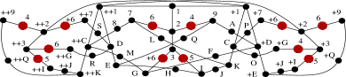
Figure 5: Bub’s MMP with 49 atoms and 36 blocks. Notice that 12 bigger dots with a pattern (red online) represent just 4 atoms: 4, 5, 6, and +6.

In Fig. 6 we show MMP hypergraph of the Conway-Kochen KS setup.Bub (1996) It reads: 123, 249, 267, 9A+D, +1CK, ++1DE, 9QE, 35I, 3+6G, EHI, IJK, CP+7, +1+D+E, CO+G, DN++7, DW++G, ++GRS, +7+V+T, S1+T, ++7TU, 1U+S, +26+9, +2+6+7, ++1+2+3, +S+W+9, +S+R+G, +34+G, +35+I, +T+U+I, +I+J+E, +9+Q+E, ++3++2+1, ++2+6++7, ++36++G, ++94++2, ++35++I, 1+1++1. It was considered to be the smallest known KS setup, but it turned out that we cannot remove atoms 7, G, Q, and others that do not share two or more blocks because they represent one of the three orientations of the spin projections.Pavičić et al. (2005); Larsson (2002) Hence, it has 51 and not 31 vectors as originally assumed. This holds for all considered KS setups. Thus, Peres’ and Bub’s setups contain 57 and 49 vectors and not both 33 as commonly assumed.

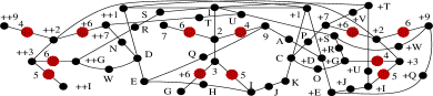
Figure 6: Conway-Kochen’s MMP. Notice that we cannot drop blocks containing ++9, ++I, 7, and G because atoms 4, 5, 6, and +6, from them also share two other blocks each. Why we cannot drop atoms 7, G, H, J, etc., is explained in the text.

Our program vectorfind gives possible values of the vectors corresponding to atoms belonging to orthogonal triples of any of the above MMPs as explained in Ref. Pavičić et al., 2005. Using our program states,Megill and Pavičić (2000) we can easily verify that all the above MMPs interpreted as lattices, even Hasse and Greechie diagrams, admit a strong set of states, and using our program latticeg,Megill and Pavičić (2000) we can prove that they all really are OMLs (by confirming that Eq. (1) is satisfied by all of them) and that they all admit Mayet vector states characterized by Eqs. (16) and (17) (by verifying that they pass in them).

On the other hand, using latticeg we can also show that if we interpret MMP hypergraph as Greechie diagrams, none of the considered lattices is modular since the modular law given by Eq. (2) fails in each of them. This might come as a surprise since Birkhoff and von Neumann Birkhoff and von Neumann (1936) proved that a finite-dimensional lattice has to be modular. However, it turns out that this is because Greechie diagrams cannot describe relations between nonorthogonal vectors and planes they span.

To understand this better we exhaustively generated Greechie lattices with up to 16 blocks and then filtered them all for modularity given by Eq. (2). For each number of blocks we find only one modular lattice—the biggest one has 33 atoms and 16 blocks. They all have star-like shape as shown in Fig. 7(a). In the figure we show the first four: 123,  123,145,  123,145,167, and 123,145,167,189—over each other—with vectors {{0,0,1}{0,1,0}{1,0,0}},  {{0,0,1}{1,-2,0}{2,1,0}},  {{0,0,1}{1,-1,0}{1,1,0}},  {{0,0,1}{1,2,0}{2,-1,0}} (over each other). And for all those lattices up to 16 blocks we generated there is always only one such star-like modular lattice among them. They all admit strong sets of states, but because of their planar distribution, they cannot describe spin vectors in a realistic spin space.

Figure 7: (a) Greechie diagrams that correspond to modular lattices with 1, 2, 3 and 4 blocks (over each other); (b) their vectors triples; (c) the smallest non-modular lattice; (d) its vector triples.

For a comparison, in Fig. 7 (c), we show the smallest OML 123,145,267, with vectors {{{0,0,1}{0,1,0}{1,0,0}}, {{0,0,1}{1,-2,0}{2,1,0}}, {{0,1,0}{1,0,-2}{2,0,1}}} shown in Fig. 7 (d), which allows a “3D” rotation that can correspond to a more complex experimental setup than the “2D” rotations given in Figs. 7 (a) and (b). This means that Greechie/Hasse diagrams cannot represent even the simplest experiment where we let a particle pass successive magnetic fields, i.e., successive Stern-Gerlach devices, mutually rotated along different axes by means of Euler angles.

The same is true of the generalized orthoarguesian equations $n$OA given by Theorem II.10 and Eq. (32) in a Hilbert space and by Theorem II.11 and Eq. (34) in a Hilbert lattice. If these equations failed in a sub-lattice, they would fail in the lattice as well. And the point here is that smallest orthoarguesian equation 3OA—and therefore all $n$OA with $n>3$—fail in almost all known KS Greechie diagrams. Peres’ fails $n$OA for $n=7$. Again, this means that we cannot represent KS setups with the help of Greechie diagrams.

The details are as follows. We consider Bub’s KS setup. To be able to apply our program vectorfind for finding the vector components of Bub’s setup shown in Fig. 5, we have to write down its MMP representation without gaps in letters. So, we have 123,…,DFH,…, where we present only those Greechie/Hasse diagrams atoms in which 3OA failed. Their Hilbert space vectors are: 1={0,0,1}, 2={1,0,0}, F={1,-2,-1}, and D={1,1,-1}.

In a Hilbert space representation, Bub’s KS setup does pass 3OA. Let us consider 3OA in the following form

$$a\perp b\quad\&\quad q\perp n\quad$$

$$\Rightarrow(a\cup b)\cap(q\cup n)\leq b\cup(a\cap(q\cup((a\cup q)\cap(b\cup n)))).$$

In 3-dim Euclidean space, all subspaces are closed (they are lines, planes, or the whole space), so $a\cup b=a+b$, i.e., subspace join and subspace sum are the same. Thus, converting joins in the previous equation to subspace sums and using the orthogonality we get:

$$a\perp b \quad\&\quad q\perp n\Rightarrow(a+b)\cap(q+n)$$

$$\leq b+(a\cap(q+((a+q)\cap(b+n)))).$$ (36)

Now, using the subspaces determined by the afore mentioned vectors and their spans in a Hilbert space we can easily check that Bub’s representation pass 3OA. For instance, vectors 1, 2, F, and D, determine subspaces {0,0,$\alpha$}, {$\beta$,0,0}, {$\gamma$,-2$\gamma$,-$\gamma$}, and {$\delta$,$\delta$,-$\delta$}, with arbitrary coefficients $\alpha,\dots$. They represent lines in both 3-dim Hilbert space and 3-dim Euclidean space. {0,0,$\alpha$}+{$\beta$,0,0}= {$\beta$,0,$\alpha$} is a plane spanned by 1 and 2, etc. We show a verification of Eq. (36) in Fig. 8.

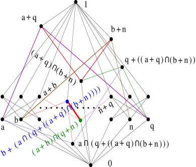
Figure 8: A new kind of lattice (MMPL) in which Bub’s setup passes 3OA. The inequality relation in Eq. (36) is represented by the thick red line.

Such a lattice—we call it MMPL—can be used for a Hilbert lattice representation of a Hilbert space setup by the following procedure. Whenever we check an equation and we need either a plane formed as a span of two existing lines or a line formed as an intersection of two existing planes, we just add them to the basic Greechie/Hasse diagram that describes the triples of orthogonal spin vectors. However, details of such a construction are not within the scope of the present paper. We will elaborate on it in a forthcoming publication and here we just give a constructive definition.

Definition III.2.

An MMPL is a lattice of setup in which we explicitly state:

1. all orthogonality relation required by the setup (spins within it);

2. only those non-orthogonal relations that are required by equations and conditions that lattice atoms of a particular setup have to satisfy for at least one set of subspace (vector) components.

So, the most general MMPL would be a lattice that would contain all possible atoms corresponding to all possible Hilbert space subspaces allowed by all possible Hilbert space conditions and equations. But our primary goal of considering MMPLs is to enable our algorithms to find minimal lattices for a particular setup which would generate just one or just a desired set of vector component values for orientation of spins and devices that would handle these spins.

Next, the superposition condition given by Eq. (18) fails in all considered KS OMLs. However, the superposition condition is a quantified expression that involves an existential quantifier, so it is possible that it passes in an enlarged lattice even though it fails in the original one. For instance, Eq. (18) fails in any five block loop but passes in the 36-36 OML shown in Fig. 11, which contains five block loops. That means that we may be able to enlarge the above KS OMLs so as to admit superposition. Of course, a first-order statement containing existential quantifiers (when expressed in prenex normal form) that holds in a lattice need not hold in a subalgebra of the lattice. As a trivial example, the statement “There exist 16 elements” is true for a 16-element lattice but false for a smaller subalgebra.

IV Lattices that Admit Almost No Hilbert Lattice Equations

There are a number of OMLs that admit a full set of states but do not admit a strong set of states and also those that admit a strong set of states (and therefore also a full set of states) but violate equations that must hold in any Hilbert lattice. Using algorithms developed in Ref. Megill and Pavičić, 2000; Pavičić and Megill, 2007 we can easily generate such lattices. For instance, a lattice with 13 atoms (one dimensional Hilbert space subspaces) and 7 blocks (connected orthogonal triples of one dimensional Hilbert space subspaces) shown in Fig. 9 (a) does admit a strong and therefore also a full set of states but violates all orthoarguesian equations. Any Hilbert lattice admits a strong and therefore a full set of states, and the orthoarguesian equations hold in any Hilbert lattice.Megill and Pavičić (2000); Pavičić and Megill (2007)

Figure 9: (a) A 13-7 OML that admits a strong set of states but violates Hilbert-space orthoarguesian equations; (b) A 16-9 OML that does not admit a strong set of states but satisfies orthoarguesian equations; (c) A 16-10 OML that admits neither a strong nor a full set of states and violates all orthoarguesian equations.

On the other hand, the 16-9 OML in Fig. 9 (b) satisfies orthoarguesian equations and admits a full set of states but does not admit a strong set of states, L42 from Fig. 2 (a) satisfies orthoarguesian equations and admits a strong set of states, but does not admit Mayet vector state Eq. (16), while 16-10 OML in Fig. 9 (c) neither admits a strong (and therefore also not a full) set of states nor satisfies the orthoarguesian equations. All these OMLs and many more provided in Refs. Megill and Pavičić, 2000; Pavičić and Megill, 2007 are examples semi-quantum lattices. Yet other examples are provided by lattices that satisfy the Godowski equations (corresponding to strong sets of states) of lower order but violate those of higher orders. Megill and Pavičić (2000) While all OMLs admitting strong sets of states satisfy all Godowski equations, there are examples showing the converse isn’t true. (Pavičić and Megill, 2007, Fig. 10, p. 780)

Such examples can be exhaustively generated, but no common structural feature has been recognized so far. To be more precise, features and general rules for generation of infinite classes of lattices that admit a strong set of states—Godowski equations,Godowski (1981); Mayet (1985, 1986, 2006); Pavičić and Megill (2007) satisfy the orthoarguesian properties—$n$OA equations,Megill and Pavičić (2000); Pavičić and Megill (2007) and a class of lattices that admit real Hilbert-space-valued states—$E_{n}$ equations, Mayet (2007); Pavičić and Megill (2007) have all been discovered, but the rule for generating all lattices that lack all these properties has not been found. Since we still do not have a single example of a complete realistic lattice for $n\geq 3$, it would be important to find a class of lattices that would narrow down the search for a complete lattice description of Hilbert space. Therefore, in Sec. VI we consider a class of OMLs that admit a field over which a Hilbert space is defined but neither a strong set of states nor any of the Hilbert space algebraic properties.

We stress here that an OML admitting a strong set of states will satisfy the Godowski equations. Godowski (1981); Mayet (1985, 1986, 2006); Pavičić and Megill (2007); Megill and Pavičić (2010) Thus OMLs that violate Godowski equations do not admit strong sets of states. Moreover, most likely they cannot be enlarged to admit such a set in order to satisfy these equations—similarly to what we have with the modular and orthoarguesian equations in Sec. III.

V MMP Hypergraphs with Equal Number of Vertices and Edges Generated from Cubic Bipartite Graphs

To avoid confusion with vertices and edges in (bipartite) graphs in this section (and only in this section) we use term atom for a vertex of a MMP hypergraph and block for an edge of an MMP hypergraph. Since later we shall consider the corresponding lattices anyway, this terminology is not inconsistent. Here we describe the exhaustive computation of MMP hypergraphs with equal numbers of atoms and blocks having 3 atoms in each block and 3 blocks containing each atom. This special case allows exploitation of a connection with graph theory in order to considerably speed up the generation compared to our earlier methods McKay et al. (2000); Pavičić et al. (2005).

We begin by representing MMP hypergraphs as graphs with two types of vertex. An atom $a$ is converted to a white vertex $A$, and a block $b$ to a black vertex $B$. If atom $a$ lies in block $b$, then vertex $A$ is joined by an edge to vertex $B$. In graph theory terminology, the resulting graph is cubic (each atom is in 3 blocks and each block has 3 atoms), and bipartite (edges have ends of different color). In Ref. Pavičić et al., 2005, Sec. 5(x) we have shown that 3-dim KS MMP hypergraphs have no loops of length less than 5. This corresponds to the graph having girth at least 10 (i.e., having no cycles of length less than 10). Apart from taking the dual MMP hypergraph, which corresponds to exchanging the colors of the vertices, isomorphism of the MMPs corresponds to isomorphism of the graphs.

For definiteness, we consider the case of 41 atoms and 41 blocks. That is, we seek 82-vertex cubic bipartite graphs of girth at least 10. The method used is an extension of one used in the non-bipartite case by McKay et al. McKay et al. (1998).

We begin with 41 white vertices and 41 black vertices, plus the 61 edges at distance at most 4 from an arbitrary fixed edge. These 61 edges form a tree, since otherwise there would be cycles of length less than 10. This starting configuration is shown in Fig. 10, with dashed lines indicating the places available for extra edges.

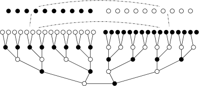
Figure 10: Starting configuration for generation of 41-41 MMPs

The task is now to add 62 extra edges so that each vertex has 3 edges and there are no short cycles. This is a non-trivial task since there are 676 places where an edge may potentially be placed, but fortunately many of the possibilities are equivalent. We proceed using a backtrack search together with some mechanisms for isomorphism rejection. The backtrack search looks for an incomplete vertex whose set of potential neighbours is as small as possible, then recursively tries each of them.

Isomorphism rejection is achieved by two methods which are described in detail in Ref. Exoo et al., 2010. First, the starting configuration has a large group of symmetries and we avoid trying more than one possibility that is equivalent under those symmetries. This can be done without explicit isomorphism testing since the structure of the starting configuration is rather simple.

Second, when the space of supergraphs of any configuration $C$ has been completely explored, we reject any future configuration $C^{\prime}$ that contains $C$ as a subgraph. This is valid since any cubic graph constructible by adding edges to $C^{\prime}$ was previously seen (up to isomorphism) when edges were added to $C$. This technique is too expensive to apply throughout the search, because subgraph finding is very difficult. As a compromise, we applied the technique only limited circumstances with at most 78 edges (the initial 61 edges plus 17 more). We did this using the graph isomorphism package nauty McKay (1990).

These isomorph-rejection methods are not complete, so each isomorphism type of graph was generated a few thousand times.

The complete search on order 41-41 involved about $10^{14}$ separate configurations and took approximately 60 GHz-years. The computation can be efficiently divided into independent parts (see Exoo et al. (2010) for an explanation), so it was run over a few weeks on a multi-processor cluster.

VI Properties of Lattices with Equal Numbers of Atoms and Blocks

In this section we consider OMLs that correspond to MMP hypergraphs we obtain by means of methods presented in the previous section.

In Ref. McKay et al., 2000 we mentioned five 35-35 OMLs (OMLs with 35 atoms and 35 blocks), eight 38-38s and gave a graphical representation of the single 36-36 (there is no 37-37). They were obtained by different algorithms and at the time we were not aware of their properties and did not yet have tools to analyze them. In  Pavičić (2009) we wrote down all 35-35s and 38-38s, gave two graphical images of them and obtained some features of them in a different context. So, in this section we shall focus on 39-39s, 40-40s, and 41-41s. In doing so, we will make use of a new way of presenting MMP hypergraphs, because our previous one becomes unreadable for so many edges. We introduce the new way as opposed to the previous one in Fig. 11.

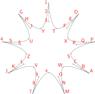
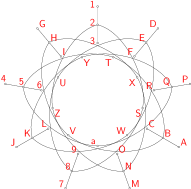
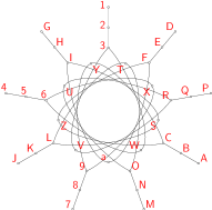
Figure 11: 36-36 OML that admits exactly one state and is dual to itself. It is given in the standard compact representation in the 1st figure and in our separate cycle representation in the other 3 figures. The figures are explained in detail in Sec. VII.

The new presentation is based on a feature of such big lattices that one can recognize separate cycles of blocks through a maximal set of vertices that belong to isolated blocks that mostly do not take part in the cycles. The terminology “isolated blocks” and “cycles” will be explained in Sec. VII. The approach stems from the way the lattice 36-36 is presented in Fig. 2 from McKay et al. (2000) which is here shown as the first figure of Fig. 11. We separately present the three cycles in the remaining three figures and see that we have three separated closed cycles. In all the other cases below we also recognize three independent cycles most of which are closed.

The cycles themselves will allow us to generate new lattice equations following the procedure developed in Megill and Pavičić (2006); Pavičić and Megill (2007); Megill and Pavičić (2010), but they do not automatically follow possible geometrical symmetries of the hypergraphs. In the 36-36 case they do, but, e.g., they do not exhibit the left right symmetry of the 35-35 lattice shown in Fig. 12. Closed cycle representation does not exhibit any symmetry.

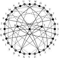
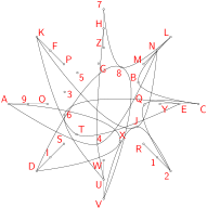
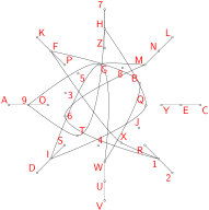
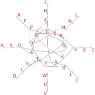
Figure 12: 1st figure shows a 35-35 lattice presented by means of its biggest loop, hexadecagon; it exhibits a left-right symmetry with respect to an axis through vertices V and Y. Three other figures show the same OML in the separate cycle representation. They are explained in detail in Sec. VII.

There are 11 eleven bipartite graphs with 78 vertices that give 39-39 OMLs. Nine of them correspond to the MMP hypergraphs that are dual to themselves—when we exchange their atoms for blocks and vice versa we obtain OMLs that are isomorphic to the original ones.

(39-39-00)

123, 145, 167, 289, 2AB, 3CD, 3EF, 4GH, 4IJ, 5KL, 5MN, 6OP, 6QR, 7ST, 7UV, 8GO, 8MV, 9Ia, 9LT, AKU, AQc, BPb, BXd, CGS, CRY, DVW, DPa, EKO, EIX, FTb, FHQ, NSc, UYZ, MRX, LWd, JWc, NZa, JYb, HZd.

(39-39-02)

123, 145, 167, 289, 2AB, 3CD, 3EF, 4GH, 4IJ, 5KL, 5MN, 6OP, 6QR, 7ST, 7UV, 8GO, 8XY, 9KQ, 9IT, AMP, AVd, BRa, BWb, CGS, CQZ, DIP, DYb, EOW, ELd, FMX, FHU, LSa, KUb, NWZ, JVZ, NTc, HRc, JXa, Ycd.

(39-39-03)

123, 145, 167, 289, 2AB, 3CD, 3EF, 4GH, 4IJ, 5KL, 5MN, 6OP, 6QR, 7ST, 7UV, 8GO, 8MU, 9IT, 9QY, AKW, AHV, BNP, BXZ, CGS, CQZ, DJP, Dac, EKO, EIX, FNY, FVb, SWd, MRd, UXa, Jbd, LTc, LZb, WYa, HRc.

(39-39-04)

123, 145, 167, 289, 2AB, 3CD, 3EF, 4GH, 4IJ, 5KL, 5MN, 6OP, 6QR, 7ST, 7UV, 8GO, 8UX, 9TZ, 9Ia, ASW, ANP, BHV, Bbc, CGS, CQa, DNX, DJb, EUY, EKZ, FIP, Fcd, KOb, MTc, LVa, MQY, HRZ, RXd, JWY, LWd.

(39-39-05)

123, 145, 167, 289, 2AB, 3CD, 3EF, 4GH, 4IJ, 5KL, 5MN, 6OP, 6QR, 7ST, 7UV, 8GO, 8XY, 9NU, 9Ra, AKW, AHQ, BMP, BVc, CGS, CNb, DVY, DIa, EKO, EJd, FHU, FXZ, LSZ, IPZ, QYd, WXb, MTd, LRc, Jbc, TWa.

(39-39-06)

123, 145, 167, 289, 2AB, 3CD, 3EF, 4GH, 4IJ, 5KL, 5MN, 6OP, 6QR, 7ST, 7UV, 8GO, 8XY, 9MQ, 9Td, AKZ, AJV, BRb, BHc, COW, CKS, DNa, DVX, EQZ, EIY, FHU, FLd, GZa, NPc, JPd, MUW, IWb, SYc, Tab, LRX.

(39-39-07)

123, 145, 167, 289, 2AB, 3CD, 3EF, 4GH, 4IJ, 5KL, 5MN, 6OP, 6QR, 7ST, 7UV, 8GO, 8MU, 9IT, 9QY, AKW, AHV, BNP, BXa, CGS, CQZ, DJP, DLd, EKO, EIX, FVY, FNc, Sab, MRb, UXZ, JWb, Tcd, WZc, LYa, HRd.

(39-39-09)

123, 145, 167, 289, 2AB, 3CD, 3EF, 4GH, 4IJ, 5KL, 5MN, 6OP, 6QR, 7ST, 7UV, 8GO, 8SX, 9NV, 9bd, AUY, AHZ, BJP, BLc, CGW, CVc, DZb, DMP, EKO, EIU, FHT, FNQ, KZa, JSa, IRb, LTd, QWa, WYd, MXY, RXc.

(39-39-10)

123, 145, 167, 289, 2AB, 3CD, 3EF, 4GH, 4IJ, 5KL, 5MN, 6OP, 6QR, 7ST, 7UV, 8GW, 8OY, 9QZ, 9IU, AKS, APb, BRa, BXc, CGX, CKQ, DMb, DJT, ESW, EZc, FLa, FIP, HVb, HZd, NOd, MRW, NUX, LVY, JYc, Tad.

Two bipartite graphs give 4 MMP hypergraphs that are not dual to themselves.

(39-39-01a)

123, 145, 167, 289, 2AB, 3CD, 3EF, 4GH, 4IJ, 5KL, 5MN, 6OP, 6QR, 7ST, 7UV, 8GO, 8SW, 9Rb, 9NX, AMP, AVZ, BHa, BQd, CKO, CUX, DQY, DJW, EIP, ETa, FRc, FLZ, GYZ, Kab, LSd, HUc, IXd, MWc, NTY, JVb.

(39-39-01b)

123, 145, 167, 289, 2AB, 3CD, 3EF, 4GH, 4IJ, 5KL, 5MN, 6OP, 6QR, 7ST, 7UV, 8GW, 8MZ, 9Sa, 9Rd, AOX, AVY, BKb, BJc, CGO, CKS, DNQ, DIU, EHY, ETc, FPZ, FLd, HRb, JPa, QWc, LVW, MTX, IXd, UZb, NYa.

(39-39-08a)

123, 145, 167, 289, 2AB, 3CD, 3EF, 4GH, 4IJ, 5KL, 5MN, 6OP, 6QR, 7ST, 7UV, 8GO, 8WX, 9JU, 9MR, ALY, AId, BVZ, BNP, CGS, CLQ, DVW, DMd, EKO, EIT, FHY, FUc, KZa, Sab, QXc, WYb, HRZ, NTX, JPb, acd.

(39-39-08b)

123, 145, 167, 289, 2AB, 3CD, 3EF, 4GH, 4IJ, 5KL, 5MN, 6OP, 6QR, 7ST, 7UV, 8GO, 8Ua, 9LT, 9Ic, ASW, AKP, BJR, BNb, CGS, CNc, DPY, DJa, EOX, ETb, FIV, FMQ, HQZ, HYb, KUZ, MWa, WXd, XZc, VYd, LRd.

The above OMLs admit neither a strong set of states nor any known property stronger than the orthomodularity itself apart from the Mayet vector field Eq. (17). One pair (39-39-01a,b) of the duals that are not dual to each other admit at least two states while the other (39-39-08a,b) admit one single state. All OMLs that are dual to themselves (39-39-00,-02–07,-09–10) admit exactly one state (1/3 for each atom).

Bipartite graphs with 80 vertices that give 40-40 OMLs are much more numerous than those with 78 vertices above. There are 174 such graphs and they give 80 OMLs that are dual to themselves. Among them there is only one (40-40-038) that admits more than one state. Among the others (94 graphs) there are eight OMLs that admit more than one state (40-40-043a,b, -097a,b, -111a,b, -130a,b).

There are 2515 bipartite graphs with 82 vertices that give 4612 41-41 OMLs. 418 of the MMP hypergraphs are dual to themselves and the other 4194 are not. The latter graphs form 2097 pairs of duals that are not dual to themselves. Of the former ones, 10 admit two or more states (all the others admit only one single state) and of the latter ones, 78 dual pairs admit two or more states and the remaining 2019 pairs admit only one state. We can recognize that the more vertices we have the smaller is the portion of lattices dual to themselves.

The biggest loops of 39-39 are enneadecagons (19-gons) and of 40-40 and 41-41 icosagons (20-gons) which makes them inappropriate for the standard graphical presentation—there are too many lines over each other in their figures to discern patterns. Therefore and because of the new feature of the existence of three separate cycles for 3D OMLs with equal number of vertices (atoms) and edges (blocks) we present details of our separate cycle representation and give several figures in the next section.

VII Separate Level Representation of the MMP Hypergraphs

As already mentioned in section VI, our new layout of MMP hypergraphs is inspired by the presentation of the 36-36 one given in Ref. McKay et al., 2000 and repeated here as the first figure in Fig. 11. Our goal is to simplify graphical representation of big MMP hypergraphs and big arbitrary hypergraphs with the same number of atoms and blocks, i.e., vertices and edges, respectively.

In the latter figure one can notice 9 radially placed blocks which do not have common atoms (and which therefore include 27 atoms), while 9 remaining atoms form an inner ring. We call radial blocks independent blocks and remaining atoms free atoms. The outermost atom of each independent block is connected to the outermost atoms of two other independent blocks by two blocks, middle atoms of which are free atoms. These connecting blocks form a cycle shown separately in the second figure of Fig. 11 (as opposed to the original layout, where oppositely placed independent blocks are connected, we connect adjacent blocks). Similarly, middle atoms of independent blocks are connected by blocks with free atoms as their middle atoms and there is again a cycle of connecting blocks (shown separately in the third figure of Fig. 11). Finally, innermost atoms of independent blocks are also connected with blocks that contain one free atom. In the original layout free atoms are “last” atoms of connecting blocks, but as the atoms in a block can be freely permuted, we can again form a cycle, shown here as the fourth figure of Fig. 11.

Based on described analysis of the layout of the 36-36 MMP, we break the representation of MMPs with equal number of atoms and blocks into three separate levels.

The first step is to identify sets of independent blocks, i.e., those that meet two criteria: they do not share atoms and no three such blocks are connected by a single block. In the archetype case of the 36-36 MMP all connecting blocks (blocks that connect independent ones) contain one free atom. When all sets of independent blocks are found, we extract the largest ones.

In the second step, for each such set we try to identify all cycles that visit all independent blocks in the set. Here we do not use the term “cycle” in the sense of graph theory—our cycle is a sequence of blocks that connect atoms of two independent blocks and pass through a free atom (if required, atoms of connecting blocks are permuted so that the free atom becomes the middle one). The shortest cycle forms the first level of our presentation. Independent blocks and free atoms are arranged in the sequence in which they are visited. But, as compared to the archetypal 36-36 MMP, there are some differences: (1) a cycle is usually not closed, that is, it does not finish in the same atom in which it starts (as can be seen on the uppermost blocks in the second figure of Fig. 12 and first ones of Figs. 13 and 14), although sometimes it does (first figure in Fig. 15); (2) in most cases some independent blocks are visited two or even three times (Figs. 12, 13, and 15); (3) in most (maybe even all) cases some free atoms are visited more than once and, of course, there are free atoms that are not visited at all (all examples). (Figs. 12, 13, 14 and 15).

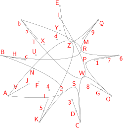
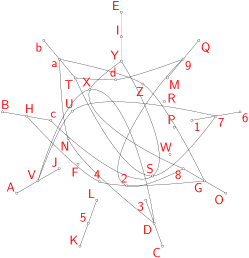
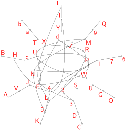
Figure 13: 39-39-06 OML dual to itself

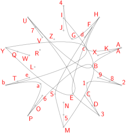
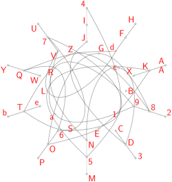
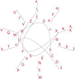
Figure 14: 40-40-34 OML dual to itself

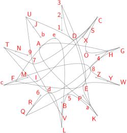
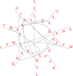
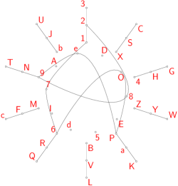
Figure 15: 40-40-38 OML dual to itself

If required—and if possible—atoms of independent blocks are permuted so that the visited atom becomes the first/outermost atom (if the block is visited twice, then visited atom is placed in the middle).

In most cases we can find a second cycle that begins and ends on the same independent block, but not in the same atom; besides, these cycles usually do not visit all independent blocks. This can be seen in all our examples: the third figure of Fig. 12 and the second figures of Figs. 13, 14 and 15. Such cycles form the second level of our layout (again, if required and if possible, atoms of independent blocks are permuted so that connecting blocks visit their second/middle atoms).

The remaining blocks are contained in the third level. In some cases they again form a cycle: the third figures of Figs. 14 and 15 (in fact, in these two examples the second and third cycles can be regarded as a single cycle, but we broke that cycle when the independent block in which it began was visited for the second time). But usually the third level contains two or even more unconnected sequences of blocks. Namely, some blocks connect one atom of some independent block and two free atoms, that is, there are some blocks that do not connect two independent blocks: the fourth figure of Fig. 12 and the third figure of Fig. 13.

The previously described parts of our algorithm are implemented in the C$++$ programming language using the Boost Graph library. Siek and Quan Lee (01) The program for the final graph layout (including the calculation of the atoms’ coordinates and drawing of the graph) is written in the Asymptote Hammerlindl et al. (08) vector graphics language based on Donald Knuth’s METAFONT.

VIII Conclusions

In this paper, we found a correct way to establish a correlation between a lattice description and a Hilbert space description of quantum systems as well as their preparation, handling, and measurement. Our description also allows for a straightforward reconstruction of the quantum formalism from empirically justified axioms. In Sec. III we explain how this can be done and why the previous descriptions from the literature were wrong. Essentially they were wrong because they were based on Greechie diagrams that handle only orthogonalities between Hilbert space subspaces and have no way to describe conditions and equations that have to be satisfied in any Hilbert space or any Hilbert lattice quantum formalism and that involve detailed relations between non-orthogonal subspaces.

We describe several families of equations and other conditions that must hold in every Hilbert lattice in Sec. II. We made use of correspondences between graphs and lattices, which in turn correspond to Hilbert space subspaces, in order to visualize and study 3-dim quantum setups in Sections III–VII. In particular, we found and investigated MMP hypergraphs (see Def. III.1) with equal numbers of vertices and edges, which correspond to bipartite graphs (Sec. V). Separately, we studied Greechie diagrams used in the literature to represent Kochen-Specker and other quantum setups (Secs. V and IV) to see which Hilbert lattice properties hold and which do not hold in them.

In Sec. III we developed a new graphical representation of the known KS setups by means of MMP hypergraphs (see Figs. 3, 4, 8, and 6) to visualize their properties. Then, using our algorithms and programs, we showed, in particular in Eq. (36) and Fig. 8, that Greechie diagrams cannot represent KS setups because they are not subalgebras of a Hilbert lattice. This is obvious from the fact that in a Greechie diagram, the join of nonorthogonal atoms (lines) $a$ and $q$ (in Fig. 8) is the whole space (1), while in a Hilbert space, it is a plane $a+q$. Therefore, if we wanted to have a lattice representation of KS setups, we should add lattice elements missing in Greechie diagrams as shown in Fig. 8. This provides us with a new type of lattices (MMPL) that include all relations—between both orthogonal and non-orthogonal elements—needed for a lattice description of a considered quantum system. We define MMPL by Def. III.2. However, a detailed elaboration of such a representation is outside of the scope of the present paper.

Application of such an approach is in any case computationally unfeasible for the time being, and therefore we consider non-quantum setups to narrow down classes of lattices that we can use to obtain complex setups in the future and in particular KS setups.

The Kochen-Specker theorem claims that there are quantum experimental setups that cannot be given a classical rendering. Its proof was based on setups (KS setups) that were considered quantum and to which it was impossible to ascribe classical 0-1 values. A number of authors have represented KS setups or indeed any spin-1 experimental setup by means of Greechie lattices.Hultgren, III and Shimony (1977); Hultgren, III (1974); Svozil and Tkadlec (1996); Svozil (1998); Tkadlec (1998, 2000, 2001); Smith (2003); Foulis (1999) However, in Sec. III we proved that no known 3-dimensional KS setup represented by Greechie/Hasse diagrams, in particular, Kochen-Specker’s, Bub’s, Conway-Kochen’s, and Peres’ pass the equations that hold in every Hilbert space. These KS setups themselves do, of course, pass these equations in the Hilbert space itself.

A Hilbert space description of such systems is ortho-isomorphic to a Hilbert lattice (Th. II.2). Beltrametti and Cassinelli (1981) An OML equipped with additional properties described in Sec. II such as admitting strong sets of states and Mayet vector states, atomicity, the superposition principle, the orthoarguesian property, etc., is easier to handle in the lattice theory than in the original Hilbert space. This is because, e.g., Peres’ KS design, shown in Fig. 4, has 40 triples of mutually orthogonal vectors. The majority of the vectors are orthogonal to vectors from other triples and rotated at various angles in space with respect to every other. We would have to extract this vector edifice from the Schrödinger equations describing the deflections of a spin-1 system in electric and magnetic fields. Lattices, as opposed to such a standard Hilbert space approach, are easier to handle, but even they are too demanding at present.

Therefore it is viable to approach the problem from the other end, to see whether we can generate lattices that would admit neither quantum nor classical interpretation from the very start (see Subsec. refsubsec:semi). Such finding of properties and lattices that are not sufficient for a full i description of a quantum system (e.g., the aforementioned description by means of Greechie diagrams) is likely to enable us to achieve, eventually, a complete lattice description (with superposition included) of quantum experiments.

Here we stress that the superposition we refer to above and in Theorem II.13 and Corollary II.13.1 is a superposition of vectors contained in 1-dim Hilbert space subspaces. As opposed to this, when we look at all possible superpositions of two vectors they span a plane in a 3-dim Hilbert space. That is trivial in the sense that for some definite constants we can always find a value that a superposition of two vectors has in particular direction, but is nontrivial in the sense that for bigger lattices we can find a superposition for vectors for which only mutual orthogonalities are known.

Another reason for a “semi-quantum approach” is that there exist several methods of finding and generating new properties and equations in the theory of OMLs and Hilbert lattices based on the lattices that do not admit some states or other properties. The most relevant here is a method of generating the Mayet-Godowski equations (Def. II.8) using lattices that do not admit strong sets of states.Pavičić and Megill (2007); Megill and Pavičić (2010) Based on all that together with several previous results based on lattices admitting only one state, Shultz (1974); Pták (1987); Weber (1994); Navara (2008) in Sec. II we formulated the following theorem:

Theorem II.13 [Semi-quantum lattice algorithms] There exist algorithms that generate finite sequences of OMLs that admit superposition, real-valued states, and a vector state given by Eq. (17) but do not admit other conditions that have to be satisfied by every Hilbert lattice, in particular equations like orthoarguesian and Godowski ones (Subsection II.2). As a consequence of violating Godowski equations, these OMLs do not admit strong sets of states.

Such a choice is determined by our recent finding that OMLs with equal number of atoms and blocks possess and lack properties stated in the theorem. They all satisfy the superposition principle and therefore do not admit classical interpretation, they all admit real-valued states, and they all admit a vector state which, when applied to Hilbert lattices, select those over which a field (real, for the time being) can be defined. They admit neither strong sets of states nor orthoarguesian properties, and this makes them non-quantum but suitable for generation of quantum properties such as Mayet-Godowski equations.Megill and Pavičić (2010) We generate them by means of novel algorithms which first generate bipartite graphs (Sec. V) and then convert them into hypergraphs that correspond to OMLs with equal numbers of atoms and blocks as described in Sec. V. These results substantiate the following corollary of Theorem II.13:

Corollary II.13.1 [Semi-quantum lattices] There exists a class of OMLs that admit superposition, real-valued states, and a vector state but do not admit other conditions that have to be satisfied by every Hilbert lattice.

To verify these and find new properties of lattices with equal number of atoms and blocks we had to generate a significant number of them. Towards that goal we developed several algorithms for generating and verifying properties on them as well as for their graphical representations, in Secs. V, VI, and VII, respectively.

The generation was performed by representing lattices as graphs then applying an extended algorithm that exhaustively determines all the associated graphs.

As a final note, we point out that in Sec. III (antepenultimate paragraph) we obtained an important “by-product” in the field of Hilbert lattice equations while we were checking whether $n$OA equations (34) pass Peres’ OML that corresponds to Peres’ MMP hypergraph shown in Fig. 4. In Ref. Megill and Pavičić, 2000, we found the new infinite class of generalized orthoarguesian equations of Theorem II.11, but at the time the computing power of available clusters were only sufficient to find lattices in which the equations up to 4OA would pass and a 5OA fail. In Ref. Pavičić and Megill, 2007 we generated lattices in which 6OA failed and OAs up to 5OA passed. Such examples are important because they prove that the equations form a successively stronger sequence at least up to those orders. In Ref. Megill and Pavičić, 2000, we proved that all individual orthoarguesian equations previously found (by other authors) were equivalent to either 3OA or 4OA. When we found our $n$OA, it was unknown whether the same might occur with $n$OA at the 6OA level.Mayet (2007) Our result (the aforementioned passing of 3OA through 6OA and failure of 7OA in Peres’ lattice) dispels any doubt. It was serendipitous that we obtained this result in this way, because no present-day supercomputer is capable of generating 7OA examples by brute force—at least not with our present algorithms.