The Mystery of the Shape Parameter IV

Abstract. This is the fourth paper of our study of the shape parameter c contained in the famous multiquadrics $(-1)^{\lceil\beta\rceil}(c^{2}+\|x\|^{2})^{\beta},\ \beta>0$, and the inverse multiquadrics $(c^{2}+\|x\|^{2})^{\beta},\ \beta<0$. The theoretical ground is the same as that of [10]. However we extend the space of interpolated functions to a more general one. This leads to a totally different set of criteria of choosing c.

keywords: radial basis function, multiquadric, shape parameter, interpolation.

1 Introduction

Again, we are going to adopt the radial function

$$h(x):=\Gamma(-\frac{\beta}{2})(c^{2}+|x|^{2})^{\frac{\beta}{2}},\ \beta\in R\backslash 2N_{\geq 0},\ c>0$$ (1)

, where $|x|$ is the Euclidean norm of $x$ in $R^{n},\ \Gamma$ is the classical gamma function, and $c,\beta$ are constants. This definition looks more complicated than the ones mentioned in the abstract. However it will simplify the Fourier transform of $h$ and our analysis of some useful results.

In order to make this paper more readable, we review some basic ingredients mentioned in the previous papers, at the cost of wasting a few pages.

For any interpolated function $f$, our interpolating function will be of the form

$$s(x):=\sum_{i=1}^{N}c_{i}h(x-x_{i})+p(x)$$ (2)

where $p(x)\in P_{m-1}$, the space of polynomials of degree less than or equal to $m-1$ in $R^{n},X=\{x_{1},\cdots,x_{N}\}$ is the set of centers(interpolation points). For $m=0,\ P_{m-1}:=\{0\}$. We require that $s(\cdot)$ interpolate $f(\cdot)$ at data points $(x_{1},f(x_{1})),\cdots,(x_{N},f(x_{N}))$. This results in a linear system of the form

$$\sum_{i=1}^{N}c_{i}h(x_{j}-x_{i})+\sum_{i=1}^{Q}b_{i}p_{i}(x_{j})=f(x_{j}) ,j=1,\cdots,N$$

$$\sum_{i=1}^{N}c_{i}p_{j}(x_{i})=0 ,j=1,\cdots,Q$$

to be solved, where $\{p_{1},\cdots,p_{Q}\}$ is a basis of $P_{m-1}$.

This linear system is solvable because $h(x)$ is conditionally positive definite(c.p.d.) of order $m=max\{\lceil\frac{\beta}{2}\rceil,0\}$ where $\lceil\frac{\beta}{2}\rceil\}$ denotes the smallest integer greater than or equal to $\frac{\beta}{2}$.

Besides the linear system, another important object is the function space. Each function of the form (1) induces a function space called native space denoted by ${\cal C}_{h,m}(R^{n})$, abbreviated as ${\cal C}_{h,m}$, where $m$ denotes its order of conditional positive definiteness. For each member $f$ of ${\cal C}_{h,m}$ there is a seminorm $\|f\|_{h}$, called the $h$-norm of $f$. The definition and characterization of the native space can be found in [4], [5], [7], [11], [12] and [14]. In this paper all interpolated functions belong to the native space.

Although our interpolated functions are defined in the entire $R^{n}$, interpolation will occur in a simplex. The definition of simplex can be found in [3]. A 1-simplex is a line segment, a 2-simplex is a triangle, and a 3-simplex is a tetrahedron with four vertices.

Let $T_{n}$ be an n-simplex in $R^{n}$ and $v_{i},\ 1\leq i\leq n+1$ be its vertices. Then any point $x\in T_{n}$ can be written as convex combination of the vertices:

$$x=\sum_{i=1}^{n+1}c_{i}v_{i},\ \sum_{i=1}^{n+1}c_{i}=1,\ c_{i}\geq 0.$$

The numbers $c_{1},\cdots,c_{n+1}$ are called the barycentric coordinates of $x$. For any n-simplex $T_{n}$, the evenly spaced points of degree $l$ are those points whose barycentric coordinates are of the form

$$(\frac{k_{1}}{l},\frac{k_{2}}{l},\cdots,\frac{k_{n+1}}{l}),\ k_{i}\ nonnegative\ integers\ with\ \sum_{i=1}^{n+1}k_{i}=l.$$

It’s easily seen that the number of evenly spaced points of degree $l$ in $T_{n}$ is exactly

$$N=dimP_{l}^{n}=\left(\begin{array}[]{c}n+l\\ n\par\par\end{array}\right)$$

where $P_{l}^{n}$ denotes the space of polynomials of degree not exceeding $l$ in n variables. Moreover, such points form a determining set for $P_{l}^{n}$, as is shown in [2].

In this paper the evaluation argument $x$ will be a point in an n-simplex, and the set $X$ of centers will be the evenly spaced points in that n-simplex.

2 Fundamental Theory

Before introducing the main theorem, we need to define two constants.

Definition 2.1

Let $n$ and $\beta$ be as in (1). The numbers $\rho$ and $\Delta_{0}$ are defined as follows.

• Suppose $\beta<n-3$. Let $s=\lceil\frac{n-\beta-3}{2}\rceil$. Then

  • if $\beta<0,\ \rho=\frac{3+s}{3}\ and\ \Delta_{0}=\frac{(2+s)(1+s)\cdots 3}{\rho^{2}};$

  • if $\beta>0,\ \rho=1+\frac{s}{2\lceil\frac{\beta}{2}\rceil+3}\ and\ \Delta_{0}=\frac{(2m+2+s)(2m+1+s)\cdots(2m+3)}{\rho^{2m+2}}$
    where $m=\lceil\frac{\beta}{2}\rceil$.

• Suppose $n-3\leq\beta<n-1$. Then $\rho=1$ and $\Delta_{0}=1$.

• Suppose $\beta\geq n-1$. Let $s=-\lceil\frac{n-\beta-3}{2}\rceil$. Then

  $$\rho=1\ and\ \Delta_{0}=\frac{1}{(2m+2)(2m+1)\cdots(2m-s+3)}\ where\ m=\lceil\frac{\beta}{2}\rceil.$$

The following theorem is the cornerstone of our theory. We cite it directly from [6] with a slight modification to make it easier to understand.

Theorem 2.2

Let $h$ be as in (1). For any positive number $b_{0}$, let $C=\max\left\{\frac{2}{3b_{0}},8\rho\right\}$ and $\delta_{0}=\frac{1}{3C}$. For any n-simplex $Q$ of diameter $r$ satisfying $\frac{1}{3C}\leq r\leq\frac{2}{3C}$(note that $\frac{2}{3C}\leq b_{0}$), if $f\in{\cal C}_{h,m}$,

$$|f(x)-s(x)|\leq 2^{\frac{n+\beta-7}{4}}\pi^{\frac{n-1}{4}}\sqrt{n\alpha_{n}}c^{\frac{\beta}{2}-l}\sqrt{\Delta_{0}}\sqrt{3C}\sqrt{\delta}(\lambda^{\prime})^{\frac{1}{\delta}}\|f\|_{h}$$ (4)

holds for all $x\in Q$ and $0<\delta<\delta_{0}$, where $s(x)$ is defined as in (2) with $x_{1},\cdots,x_{N}$ the evenly spaced points of degree $l$ in $Q$ satisfying $\frac{1}{3C\delta}\leq l\leq\frac{2}{3C\delta}$. The constant $\alpha_{n}$ denotes the volume of the unit ball in $R^{n}$, and $0<\lambda^{\prime}<1$ is given by

$$\lambda^{\prime}=\left(\frac{2}{3}\right)^{\frac{1}{3C}}$$

which only in some cases mildly depends on the dimension n.

Remark:(a)Note that the right-hand side of (4) approaches zero as $\delta\rightarrow 0^{+}$. This is the key to understanding Theorem2.2. The number $\delta$ is in spirit equivalent to the well-known fill-distance. Although the centers $x_{1},\cdots,x_{N}$ are not purely scattered, the shape of the simplex is controlled by us. Hence the distribution of the centers is practically quite flexible. (b)In (4) the shape parameter c plays a crucial role and greatly influences the error bound. This provides us with a theoretical ground of choosing the optimal c. However we need further work before presenting useful criteria.

In this paper all interpolated functions belong to a kind of space defined as follows.

Definition 2.3

For any positive number $\sigma$,

$$E_{\sigma}:=\left\{f\in L^{2}(R^{n}):\ \int|\hat{f}(\xi)|^{2}e^{\frac{|\xi|^{2}}{\sigma}}d\xi<\infty\right\}$$

where $\hat{f}$ denotes the Fourier transform of $f$. For each $f\in E_{\sigma}$, its norm is

$$\|f\|_{E_{\sigma}}:=\left\{\int|\hat{f}(\xi)|^{2}e^{\frac{|\xi|^{2}}{\sigma}}d\xi\right\}^{1/2}$$

.

The following lemma is cited from [9].

Lemma 2.4

Let $h$ be as in (1). For any $\sigma>0$, if $\beta<0$, $|n+\beta|\geq 1$ and $n+\beta+1\geq 0$, then $E_{\sigma}\subseteq{\cal C}_{h,m}(R^{n})$ and for any $f\in E_{\sigma}$, the seminorm $\|f\|_{h}$ of $f$ satisfies

$$\|f\|_{h}\leq 2^{-n-\frac{1+\beta}{4}}\pi^{-n-\frac{1}{4}}c^{\frac{1-n-\beta}{4}}\left\{(\xi^{*})^{\frac{n+\beta+1}{2}}e^{c\xi^{*}-\frac{(\xi^{*})^{2}}{\sigma}}\right\}^{1/2}\|f\|_{E_{\sigma}}$$

where

$$\xi^{*}:=\frac{c\sigma+\sqrt{c^{2}\sigma^{2}+4\sigma(n+\beta+1)}}{4}$$

.

Corollary 2.5

Under the conditions of Theorem2.2, if $f\in E_{\sigma},\ \beta<0,\ |n+\beta|\geq 1$ and $n+\beta+1\geq 0$, (4) can be transformed into

$$|f(x)-s(x)|\leq 2^{-\frac{3n}{4}-2}\pi^{-\frac{3}{4}n-\frac{1}{2}}\sqrt{n\alpha_{n}}\sqrt{\Delta_{0}}\sqrt{3C}c^{\frac{\beta-n+1-4l}{4}}\left\{(\xi^{*})^{\frac{n+\beta+1}{2}}e^{c\xi^{*}-\frac{(\xi^{*})^{2}}{\sigma}}\right\}^{1/2}\sqrt{\delta}(\lambda^{\prime})^{\frac{1}{\delta}}\|f\|_{E_{\sigma}}$$ (5)

where

$$\xi^{*}:=\frac{c\sigma+\sqrt{c^{2}\sigma^{2}+4\sigma(n+\beta+1)}}{4}$$

.

Proof. This is an immediate result of Theorem2.2 and Lemma2.4.                                             $\sharp$

Note that Corollary2.5 covers the very useful case $\beta=-1,\ n\geq 2$. However the case $\beta=-1,\ n=1$ is excluded. For this case we need a different approach.

Lemma 2.6

Let $\sigma>0,\ \beta=-1$ and $n=1$. For any $f\in E_{\sigma}$,

$$\|f\|_{h}\leq 2^{-(n+\frac{1}{4})}\pi^{-1}\left\{\frac{1}{ln2}+2\sqrt{3}M(c)\right\}^{1/2}\|f\|_{E_{\sigma}}$$

where $M(c):=e^{1-\frac{1}{c^{2}\sigma}}$ if $c\leq\frac{2}{\sqrt{3\sigma}}$ and $M(c):=g(\frac{c\sigma+\sqrt{c^{2}\sigma^{2}+4\sigma}}{4})$ if $c>\frac{2}{\sqrt{3\sigma}}$, where $g(\xi):=\sqrt{c\xi}e^{c\xi-\frac{\xi^{2}}{\sigma}}$.

Proof. This is just Theorem2.5 of [9].                                                                               $\sharp$

Corollary 2.7

Let $\sigma>0,\ \beta=-1$ and $n=1$. Under the conditions of Theorem2.2, if $f\in E_{\sigma}$, (4) can be transformed into

$$|f(x)-s(x)|\leq 2^{\frac{\beta-3n}{4}-2}\pi^{\frac{n-5}{4}}\sqrt{n\alpha_{n}}\sqrt{\Delta_{0}}\sqrt{3C}c^{\frac{\beta}{2}-l}\left\{\frac{1}{ln2}+2\sqrt{3}M(c)\right\}^{1/2}\sqrt{\delta}(\lambda^{\prime})^{\frac{1}{\delta}}\|f\|_{E_{\sigma}}$$ (6)

where $M(c)$ is defined as in Lemma2.6.

Proof. This is an immediate result of Theorem2.2 and Lemma2.6.                                           $\sharp$

Now we have dealt with the most useful cases for $\beta<0$. The next step is to treat $\beta>0$.

Lemma 2.8

Let $\sigma>0,\ \beta>0$ and $n\geq 1$. For any $f\in E_{\sigma}$,

$$\|f\|_{h}\leq d_{0}c^{\frac{1-\beta-n}{4}}\left\{\frac{(\xi^{*})^{\frac{1+\beta+n}{2}}e^{c\xi^{*}}}{e^{\frac{(\xi^{*})^{2}}{\sigma}}}\right\}^{1/2}\|f\|_{E_{\sigma}}$$

where $\xi^{*}=\frac{c\sigma+\sqrt{c^{2}\sigma^{2}+4\sigma(1+\beta+n)}}{4}$ and $d_{0}$ is a constant depending on $n,\ \beta$ only.

Proof. This is just Theorem2.8 of [9].                                                                              $\sharp$

Corollary 2.9

Let $\sigma>0,\ \beta>0$ and $n\geq 1$. If $f\in E_{\sigma}$, (4) can be transformed into

$$|f(x)-s(x)|\leq 2^{\frac{n+\beta-7}{4}}\pi^{\frac{n-1}{4}}\sqrt{n\alpha_{n}}\sqrt{\Delta_{0}}\sqrt{3C}d_{0}c^{\frac{1+\beta-n-4l}{4}}\left\{\frac{(\xi^{*})^{\frac{1+\beta+n}{2}}e^{c\xi^{*}}}{e^{\frac{(\xi^{*})^{2}}{\sigma}}}\right\}^{1/2}\sqrt{\delta}(\lambda^{\prime})^{\frac{1}{\delta}}\|f\|_{E_{\sigma}}$$ (7)

where $d_{0},\ \xi^{*}$ are as in Lemma2.8.

Proof. This is an immediate result of Theorem2.2 and Lemma2.8.                                         $\sharp$

3 Criteria of Choosing c

Note that in (5),(6) and (7), there is a main function of c. As in [9], let’s call this function the MN function, denoted by $MN(c)$, and its graph the MN curve. The optimal choice of c is then the number minimizing $MN(c)$. However, unlike [9], the range of c is the entire interval $(0,\infty)$, rather than a proper subset of $(0,\infty)$.

We now begin our criteria.

Case1. $\beta<0,\ |n+\beta|\geq 1$ and $n+\beta+1\geq 0$ Let $f\in E_{\sigma}$ and $h$ be as in (1). Under the conditions of Theorem2.2, for any fixed $\delta$ satisfying $0<\delta<\delta_{0}$, the optimal value of c in $(0,\infty)$ is the number minimizing

$$MN(c):=c^{\frac{\beta-n+1-4l}{4}}\left\{(\xi^{*})^{\frac{n+\beta+1}{2}}e^{c\xi^{*}-\frac{(\xi^{*})^{2}}{\sigma}}\right\}^{1/2}$$

where

$$\xi^{*}=\frac{c\sigma+\sqrt{c^{2}\sigma^{2}+4\sigma(n+\beta+1)}}{4}$$

.

Reason: This is a direct consequence of (5).                                                                       $\sharp$

Remark:(a)It’s easily seen that $MN(c)\rightarrow\infty$ as $c\rightarrow\infty$. Also, if $n+\beta+1>0,\ MN(c)\rightarrow\infty$ as $c\rightarrow 0^{+}$. (b)Case1 covers the frequently seen case $\beta=-1,\ n\geq 2$. (c)The number c minimizing $MN(c)$ can be easily found by Mathematica or Matlab.

Numerical Results:

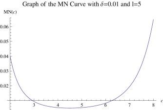
Figure 1: Here $n=2,\beta=-1,\sigma=1$ and $b_{0}=1$.

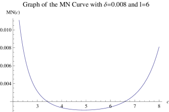
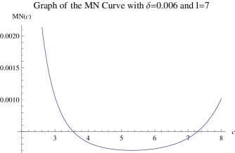
Figure 2: Here $n=2,\beta=-1,\sigma=1$ and $b_{0}=1$.

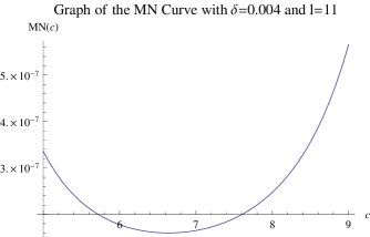
Figure 3: Here $n=2,\beta=-1,\sigma=1$ and $b_{0}=1$.

Figure 4: Here $n=2,\beta=-1,\sigma=1$ and $b_{0}=1$.

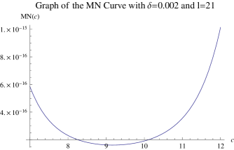
Figure 5: Here $n=2,\beta=-1,\sigma=1$ and $b_{0}=1$.

Case2. $\beta=-1$ and $n=1$ Let $f\in E_{\sigma}$ and $h$ be as in (1). Under the conditions of Theorem2.2, for any fixed $\delta$ satisfying $0<\delta<\delta_{0}$, the optimal value of c in $(0,\infty)$ is the number minimizing

$$MN(c):=c^{\frac{\beta}{2}-l}\left\{\frac{1}{ln2}+2\sqrt{3}M(c)\right\}^{1/2}$$

where

$$M(c):=\left\{\begin{array}[]{ll}e^{1-\frac{1}{c^{2}\sigma}}&\mbox{if $0<c\leq\frac{2}{\sqrt{3\sigma}}$,}\\ g(\frac{c\sigma+\sqrt{c^{2}\sigma^{2}+4\sigma}}{4})&\mbox{if $\frac{2}{\sqrt{3\sigma}}<c$}\par\end{array}\right.$$

, $g$ being defined by $g(\xi):=\sqrt{c\xi}e^{c\xi-\frac{\xi^{2}}{\sigma}}$.

Reason: This is a direct result of (6).                                                                               $\sharp$

Remark: Note that $MN(c)\rightarrow\infty$ both as $c\rightarrow\infty$ and $c\rightarrow 0^{+}$. Now let’s see some numerical examples.

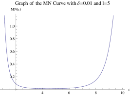
Figure 6: Here $n=1,\beta=-1,\sigma=1$ and $b_{0}=1$.

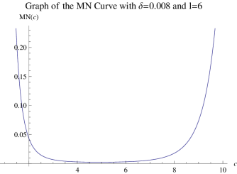
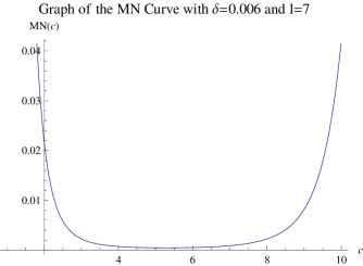
Figure 7: Here $n=1,\beta=-1,\sigma=1$ and $b_{0}=1$.

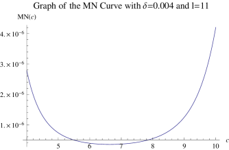
Figure 8: Here $n=1,\beta=-1,\sigma=1$ and $b_{0}=1$.

Figure 9: Here $n=1,\beta=-1,\sigma=1$ and $b_{0}=1$.

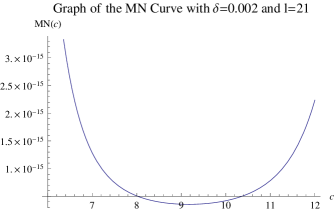
Figure 10: Here $n=1,\beta=-1,\sigma=1$ and $b_{0}=1$.

Case3. $\beta>0$ and $n\geq 1$ Let $f\in E_{\sigma}$ and $h$ be as in (1). Under the conditions of Theorem2.2, for any fixed $\delta$ satisfying $0<\delta<\delta_{0}$, the optimal value of c in $(0,\infty)$ is the number minimizing

$$MN(c):=c^{\frac{1+\beta-n-4l}{4}}\left\{\frac{(\xi^{*})^{\frac{1+\beta+n}{2}}e^{c\xi^{*}}}{e^{\frac{(\xi^{*})^{2}}{\sigma}}}\right\}^{1/2}$$

, where

$$\xi^{*}=\frac{c\sigma+\sqrt{c^{2}\sigma^{2}+4\sigma(1+\beta+n)}}{4}$$

.

Reason: This follows from (7).                                                                                        $\sharp$

Remark: By observing that

$$c\xi^{*}-\frac{(\xi^{*})^{2}}{\sigma}=\frac{1}{16}\left[2c^{2}\sigma+2c\sqrt{c^{2}\sigma^{2}+4\sigma(n+\beta+1)}-(4n+\beta+1)\right]$$

, we can easily obtain useful results as follows. (a)If $1+\beta-n-4l>0$, $\lim_{c\rightarrow 0^{+}}MN(c)=0$. (b)If $1+\beta-n-4l<0,\ \lim_{c\rightarrow 0^{+}}MN(c)=\infty$. (c)If $1+\beta-n-4l=0,\ \lim_{c\rightarrow 0^{+}}MN(c)$ is a finite positive number. (d)$\lim_{c\rightarrow\infty}MN(c)=\infty$.

Numerical Results: For simplicity, we offer results for $n=1$ only. In fact for $n\geq 1$ similar results can be presented without slight difficulty.

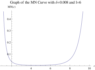
Figure 11: Here $n=1,\beta=1,\sigma=1$ and $b_{0}=1$.

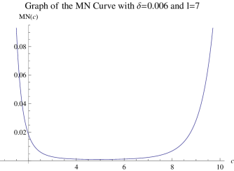
Figure 12: Here $n=1,\beta=1,\sigma=1$ and $b_{0}=1$.

Figure 13: Here $n=1,\beta=1,\sigma=1$ and $b_{0}=1$.

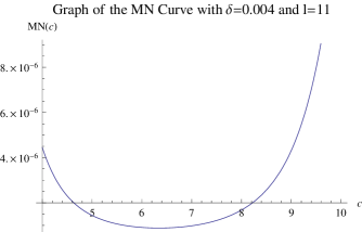
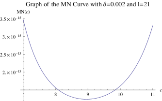
Figure 14: Here $n=1,\beta=1,\sigma=1$ and $b_{0}=1$.

Figure 15: Here $n=1,\beta=1,\sigma=1$ and $b_{0}=1$.

References

[1]Abramowitz and Segun,
Handbook of Mathematical Functions,
Dover Publications, INC., New York.
[2]L.P. Bos,
Bounding the Lebesgue function for Lagrange interpolation in a simplex,
J. Approx. Theory, 38(1983)43-59.
[3]W. Fleming,
Functions of Several Variables, Second Edition,
Springer-Verlag, 1977.
[4]L.T. Luh,
The Equivalence Theory of Native Spaces,
Approx. Theory Appl. (2001), 17:1, 76-96.
[5]L.T. Luh,
The Embedding Theory of Native Spaces,
Approx. Theory Appl. (2001), 17:4, 90-104.
[6]L.T. Luh,
An Improved Error Bound for Multiquadric Interpolation,
Inter. J. Numeric. Methods Appl. Vol. 1, No.2, pp. 101-120, 2009.
[7]L.T. Luh,
On Wu and Schaback’s Error Bound,
Inter. J. Numeric. Methods Appl. Vol. 1, No2, pp. 155-174, 2009.
[8]L.T. Luh,