Quantum flavor oscillations extended to the Dirac theory

Abstract

Flavor oscillations by itself and its coupling with chiral oscillations and/or spin-flipping are the most relevant quantum phenomena of neutrino physics. This report deals with the quantum theory of flavor oscillations in vacuum, extended to fermionic particles in the several subtle aspects of the first quantization and second quantization theories. At first, the basic controversies regarding quantum-mechanical derivations of the flavor conversion formulas are reviewed based on the internal wave packet (IWP) framework. In this scenario, the use of the Dirac equation is required for a satisfactory evolution of fermionic mass-eigenstates since in the standard treatment of oscillations the mass-eigenstates are implicitly assumed to be scalars and, consequently, the spinorial form of neutrino wave functions is not included in the calculations. Within first quantized theories, besides flavor oscillations, chiral oscillations automatically appear when we set the dynamic equations for a fermionic Dirac-type particle. It is also observed that there is no constraint between chiral oscillations, when it takes place in vacuum, and the process of spin-flipping related to the helicity quantum number, which does not take place in vacuum. The left-handed chiral nature of created and detected neutrinos can be implemented in the first quantized Dirac theory in presence of mixing; the probability loss due to the changing of initially left-handed neutrinos to the undetected right-handed neutrinos can be obtained in analytic form. These modifications introduce correction factors proportional to $m_{\nu}^{\mbox{\tiny$2$}}/E_{\nu}^{\mbox{\tiny$2$}}$ that are very difficult to be quantified by the current phenomenological analysis. All these effects can also be identified when the non-minimal coupling with an external (electro)magnetic field in the neutrino interacting Lagrangian is taken into account. In the context of a causal relativistic theory of a free particle, one of the two effects should be present in flavor oscillations: (a) rapid oscillations or (b) initial flavor violation. Concerning second quantized approaches, a simple second quantized treatment exhibits a tiny but inevitable initial flavor violation without the possibility of rapid oscillations. Such effect is a consequence of an intrinsically indefinite but approximately well defined neutrino flavor. Within a realistic calculation in pion decay, including the quantum field treatment of the creation process with finite decay width, it is possible to quantify such violation. The violation effects are shown to be much larger than loop induced lepton flavor violation processes, already present in the standard model in the presence of massive neutrinos with mixing. For the implicitly assumed fermionic nature of the Dirac theory, the conclusions of this report lead to lessons concerning flavor mixing, chiral oscillations, interference between positive and negative frequency components of Dirac equation solutions, and the field formulation of quantum oscillations.

I Introduction

Particle mixing and flavor oscillations Gel55 ; Pic55 ; Gri69 ; Bil76 ; Fri76 continue to stimulate interesting and sometimes fascinating discussions on the many subtleties of quantum mechanics involved in oscillation phenomena Zra98 ; akhmedov:paradoxes ; glashow:no . The flavor mixing models Nir03 , the quantum field prescriptions Kob82 ; Bla95 ; Beu03 ; Giu02 ; GiuBla ; Bla03 ; akhmedov:qft and, generically, the quantum mechanics of oscillation phenomena Giunti:91 ; Ber08B ; Ber08A ; Vog04 ; Giu98 ; Ber05 ; Akh10 have been extensively studied in the last years. In particular, the properties of neutrinos Zub98 ; Alb03 obtained in all of these frameworks have become the subject of an increasing number of theoretical constructions. Notwithstanding the exceptional ferment in this field, the numerous conceptual difficulties in describing accurately the particle mixing and oscillations have renewed the interest in understanding the derivation of the flavor conversion probability formulas and in overcoming the main physical inconsistencies hidden in the standard theoretical approaches.

The flavor oscillation analysis have been supported by compelling experimental evidences which have continuously ratified that neutrinos undergo flavor oscillations in vacuum and in matter. One can focus, for instance, on the outstanding results of the Super-Kamiokande atmospheric neutrino experiment Fuk02 , in which a significant up-down asymmetry of the high-energy muon events was observed, the results of the SNO solar neutrino experiment Ahm02 ; Ban03 , in which a direct evidence for the transition of the solar electron neutrinos into other flavors was obtained, and also the results of the KamLAND experiment Egu03 that confirmed that the disappearance of solar electron neutrinos is mainly due to oscillations among active neutrinos and not due to other types of neutrino conversion mechanisms Guz02 ; Bar02B . The experimental data could be completely interpreted and understood in terms of three neutrino flavors, with the exception of the LSND anomaly Ban03 ; Ana98 ; Agu01 . Such anomaly, although not confirmed by the MiniBoone experiment Agu07 ; miniboone:prl09 , led to speculations of the existence of (at least) a fourth light neutrino flavor which had to be inert. The presence of such light sterile neutrinos is largely excluded by the oscillation data minos:10 ; miniboone:sterile but depending on their mass scale it may influence certain astrophysical and cosmological phenomena ranging from the thermal evolution of the Universe wmap:10 to supernova explosion, pulsar kicks and even a significant part of dark matter kusenko:09 . On the other hand, the hypothesis of mixing between known neutrino species (electron, muon and tau) and higher mass neutrinos has much stronger theoretical motivation since it may account for the lightness of the active neutrinos through the seesaw mechanism Gel79 ; Ma:prl98 and also account for the matter and antimatter asymmetry of the Universe through the mechanism of leptogenesis leptog . The observation of such mixing at low energies, however, could be extremely difficult.

In parallel, the neutrino spin-flipping attributed to some dynamic external Oli90 interacting process, which comes from the non-minimal coupling of a magnetic moment with an external electromagnetic field Vol81 , was formerly supposed to be a relevant effect in the context of the solar-neutrino puzzle. As a consequence of a non-vanishing magnetic moment interacting with an external electromagnetic field, left-handed neutrinos could change their helicity (to right-handed)Bar96 . The effects on flavor oscillations due to external magnetic interactions in a kind of chirality-preserving phenomenon were also studied Oli96 but they lack a full detailed theoretical analysis. It was partially provided by some recent theoretical studies where the Dirac/Majorana characteristic of neutrinos becomes relevant Ber08A ; Dvo09 ; Dvo02 ; Bla09 . Only for ultra-relativistic (UR) neutrinos, however, changing helicity approximately means changing chirality. One of our goals is to demonstrate that, in the context of oscillation phenomena and in the framework of a first quantized theory, the small differences between the concepts of chirality and helicity, which had been interpreted as representing the same physical quantities for massless particles Oli90 ; Vol81 ; Bar96 ; Oli96 ; Kim93 ; DeL98 ; Dvo02 , can be quantified for massive particles. It raises the possibility that chirality coupled to flavor oscillations could lead to some small modifications to the standard flavor conversion formula Ber05 .

On the theoretical background, under the point of view of a first quantized theory, the treatment of the flavor oscillation phenomena in terms of the intermediate wave packet (IWP) approach Kay81 eliminates the most controversial points arising with the standard plane-wave formalism Kay89 ; Kay04 . However, a common argument against the IWPs is that oscillating neutrinos are neither prepared nor observed Beu03 . This point was partially clarified by Giunti Giu02 who suggested a solution in terms of an improved version of the IWP model where the wave packet (WP) of the oscillating particle is explicitly computed with field-theoretical methods by means of the external wave packet (EWP) approach Kob82 ; Beu03 .

Such approach, in contrast to IWP approaches, became the customary way to avoid the ambiguities involving the question on how neutrinos are created and detected. According to Ref. Beu03 , the IWP treatments are the simpler first quantized ones treating the propagation of neutrinos as free localized wave packets. In contrast, EWP approaches consider localized wave packets for the sources and detection particles while the neutrinos were considered intermediate virtual particles.

On the other hand, another classification scheme can be used do classify the various existing treatments considering a more physical criterion irrespective of the use of wave packets. It refers to the descriptions of neutrino oscillations that (A) include explicitly the interactions responsible for the mixing and those (B) that only treat the propagation of neutrinos, i. e., the mixing is an ad hoc ingredient. A more subtle aspect in between would be the (explicit or phenomenologically modeled) consideration of the production (and detection) process(es). In general, the IWP approaches are of type (B). The EWP approaches are of type (A). The Blasone and Vitiello approach Bla95 , although in the quantum field theory (QFT), is of type (B) since mixing is introduced without explicitly including the interaction responsible for it. The type (B) approaches have the virtue that they can be formulated in a way in which total oscillation probability in time is always conserved and normalized to unity DeL04 ; Bla95 ; Ber04 ; Ber04B ; ccn:no12 . This feature will be present in all first quantized approaches treated here (sections II and  III) and in a second quantized version (section V.1). If different observables are considered, or a modeling of the details of the production and detection processes is attempted, further normalization is necessary Giunti:91 ; Giu98 ; BlasoneP:03 . In such cases, the oscillating observable might differ from the oscillation probability. On the other hand, type (A) approaches tend to be more realistic and can account for the production and detection processes giving experimentally observable oscillation probabilities Cardall.00 . Of course, they are essential to the investigation of how neutrinos are produced and detected Kie96 ; Kie97 ; Dolgov . To rigorously derive a flavor/chiral conversion formula for fermionic particles (non-minimally coupled to an external magnetic field), we avoid the field theoretical methods in the preliminary investigation. As we are initially interested in the Dirac equation properties, as a first analysis, the IWP framework is a suitable simplification for the understanding of the physical aspects concerning the oscillation phenomena.

In section II of this manuscript, the spatial localization is included in the formulation of flavor oscillations. Quite generally, the analytical description of the dynamical evolution of a mass-eigenstate do not involve the wave packet limitations. In particular, the analytical properties of gaussian distributions Giu98 ; Giu02 enable us to quantify the first and the second order corrections to the oscillating behavior of propagating particles. We assume sharply peaked momentum distributions and then we approximate the mass-eigenstate energy in order to analytically obtain the expressions for the wave packet time evolution and for the flavor oscillation probability. In the IWP approach a consistent energy expansion is taken up to the second order term in the wave packet parameter $\sigma_{\mbox{\tiny$i$}}\sim(a\,E_{\mbox{\tiny$i$}})^{-1}$, that satisfies $\sigma_{\mbox{\tiny$i$}}\ll 1$ for sharply peaked momentum distributions. The wave packet spreading as well as the loss of coherence between the propagating wave packets are quantified in both non-relativistic (NR) and ultra-relativistic (UR) propagation regimes. Thus, the preliminary step of our study consists in a self-consistent approximation to the mass-eigenstate energy in order to analytically obtain the expressions for the wave packet time evolution and for the flavor oscillation probability. We also identify an additional time-dependent phase which changes the standard oscillating character of the flavor conversion formula.

The extension to the Dirac theory is introduced in section III, where spin and relativistic completeness are included into the flavor oscillation formulation. This section is concerned with the analytical derivation of a flavor conversion formula where the fermionic instead of the scalar character of a propagating mass-eigenstate is assumed. To that end we shall use the Dirac equation as the evolution equation for the mass-eigenstates and show that the Dirac formalism is useful and essential in keeping clear many of the conceptual aspects of quantum oscillation phenomena that naturally arise in a relativistic spin one-half particle theory. More particularly, we show that a superposition of both positive and negative frequency solutions of the Dirac equation is often a necessary condition to correctly describe the time evolution of the mass-eigenstate wave packets. We give, for strictly peaked momentum distributions and UR particles, an analytic expression for the Dirac flavor conversion probability. A modified formula for the conversion probability is shown and an additional rapid oscillation term, coming from the interference between the positive and negative frequency contributions, is found. To completely disentangle the influence of the initial wave packet to the phenomenon, an analysis independent of the initial wave packet is conducted through the calculation of the Dirac time evolution kernel in the presence of flavor mixing. The properties of completeness and causality are briefly analyzed. An analogous calculation is performed for relativistic spin zero particles to show that rapid oscillations are indeed a consequence of the presence of positive and negative frequency solutions (completeness) for relativistic wave equations and not of the spin degree of freedom itself. Within first quantized Dirac theory, we also establish the inextricable relationship between two phenomena: initial flavor violation and rapid oscillations.

Further consequences of spin structure and relativistic completeness, such as chiral oscillations, are discussed in section IV. Chiral oscillations naturally enter the discussion of neutrino oscillations because neutrinos are produced and detected through weak interactions that are chiral in nature, more specifically, left-handed in chirality. It is shown that the inclusion of chiral oscillation effects, together with the time-evolution of spinorial wave packets for the mass-eigenstates, can modify the flavor conversion probability formula. In particular, the probability loss due to the conversion of left-handed to right-handed neutrinos is calculated. The differences between the dynamics of chirality and helicity for a neutrino non-minimally coupled to an external (electro)magnetic field are expressed in terms of the equation of the motion of the correspondent operators $\gamma^{\mbox{\tiny$5$}}$ and $h$, respectively. In particular, the oscillating effects can be explained as an implication of the zitterbewegung (ZBW) phenomenon that emerges when the Dirac equation solution is used for describing the time evolution of a wave packet Ber04 . Due to this tenuous relation between ZBW and chiral oscillations, the question to be analyzed in this section concerns with the immediate description of chiral oscillations in terms of the ZBW motion, i. e., we shall demonstrate that, in fact, chiral oscillations are coupled with the ZBW motion so that they cannot exist independently of each other. It provides the interpretation of chiral oscillations as very rapid oscillations in position along the direction of motion, i.e., longitudinal to the momentum of the particle. In a subsequent step, we report about a further class of static properties of neutrinos, namely, the (electro)magnetic moment associated to the Lagrangian with non-minimal coupling. It allows the comparison between the dynamics of chiral oscillations and the dynamics of spin-flipping in the presence of an external magnetic field. It is also verified how the interaction with an external (electro)magnetic field can modify the neutrino flavor oscillation formula Ber04B . To summarize, the basic idea is thus to quantify the modifications that appear in the flavor-chirality conversion formula, previously obtained for free propagating particles in vacuum Ber05 , when an external magnetic field can affect chiral oscillations.

In section V we finally analyze the inclusion of some aspects of field quantization into the description. Firstly, a simple second quantized description of the flavor oscillation phenomenon is devised based on free second quantized Dirac theory. There is no interference term between positive and negative components, but it still gives simple normalized oscillation probabilities. We also review the central issue distinguishing the general IWP and EWP Beu03 ; Giu93 approaches: despite its direct unobservability, is the intermediate neutrino a real (on-shell) particle propagating freely? The answer is affirmative except for the possibility of contribution of the antineutrino component in the propagation of virtual neutrinos which, nevertheless, is very small ccn:no12 . Thus IWP description is a good approximation of the oscillation phenomenon ccn:no12 ; Gri96 . We also compare the distinct approach of Blasone and Vitiello Bla95 with the first quantized description of neutrino oscillations.

We have also considered that a central issue of the phenomenon of flavor oscillations discussed along our manuscript is: how the coherent superposition of mass-eigenstate neutrinos, i. e., the flavor state, is created and detected Dolgov ; Kie97 ; Ric93 ? To answer such question, it is necessary to explicitly consider the interactions responsible for creation and/or detection. Our contribution to such a fruitful discussion is a detailed calculation of the creation probability of the neutrino produced through pion decay performed using the full (perturbative) QFT formalism at tree level, with explicit inclusion of pion localization. As a result, it is possible to study how the localization properties of neutrinos follows from the parent particle (pion) that decays. The calculation then provides the missing ingredients to quantify the new effect of intrinsic neutrino flavor violation ccn:intrinsic . Such effect is already present in first quantized formulations and it is manifested as an initial flavor violation or flavor indefinition but its presence was not mandatory and its magnitude could not be calculated a priori DeL04 . Moreover, we can show that the coherent creation of neutrino flavor states follows from the common negligible contribution of neutrino masses to their creation probabilities. At the same time, in the strict sense, we can also conclude that neutrino flavor is only an approximately well defined concept.

The manuscript is structured in order to allow the reader to recognize the origin of each novel ingredient that can be included in the description of the quantum flavor oscillation phenomenon for neutrinos. We draw our conclusions in section VI.

II Inclusion of spatial localization

This section deals with the quantum-mechanical derivation of the oscillation formula, as well as the inclusion of spatial localization through the IWP framework, as it has been extensively discussed in the literature Kay89 ; Kay04 ; Zra98 ; Beu03 . Our main contribution concerns the identification, through analytical expressions, of secondary effects coupled with the wave packet decoherence, which introduce small modifications to the oscillation pattern. In particular, a preliminary discussion introducing the possibility of initial flavor violation and the respective consequences at neutrino creation/propagation/detection, is contextualized in the IWP framework.

Associating a plane wave with each mass-eigenstate Kay89 ; Kay04 is certainly the simplest and probably the most intuitive way to describe the interference phenomenon that gives rise to flavor oscillations in terms of an oscillation length and an oscillation probability. For oscillations between two different neutrino flavors that we will choose to be ${\nu_{e}}$ and ${\nu_{\mu}}$ by convenience, the probability for flavor transition is usually expressed in terms of the mixing angle $\theta$ and of the relative phase $\Delta\Phi$ by

$$\mathcal{P}(\bm{{\nu_{e}}}\rightarrow\bm{{\nu_{\mu}}})=\sin^{\mbox{\tiny$2$}}(2\theta)\,\sin^{\mbox{\tiny$2$}}\left[\frac{\Delta\Phi}{2}\right]$$ (1)

where the Lorentz invariant phase difference,

$$\Delta\Phi=\Delta\,(E\,T-p\,L),$$ (2)

sets that initial pure flavor states are modified with time and distance. The mass-eigenstate phase difference $\Delta\Phi$ is then conventionally evaluated by setting $\Delta T=\Delta L=0$ and considering, for ultra-relativistic (UR) particles, $T\approx L$ and $p_{\mbox{\tiny$1$},\mbox{\tiny$2$}}\approx E_{\mbox{\tiny$1$},\mbox{\tiny$2$}}$, i. e.

$$\Delta\Phi=T\,\Delta E-L\,\Delta p\approx L\,\left(\Delta E-\Delta p\right)\approx\frac{\Delta m^{\mbox{\tiny$2$}}}{2\bar{p}}\,L.$$ (3)

One thus gets the well-known expression Kay04

$$\mathcal{P}(\bm{{\nu_{e}}}\rightarrow\bm{{\nu_{\mu}}};L)=\sin^{\mbox{\tiny$2$}}(2\theta)\sin^{\mbox{\tiny$2$}}\left[\frac{\Delta m^{\mbox{\tiny$2$}}}{4\bar{p}}\,L\right].$$ (4)

Considering the plane wave approach, controversial points arises even in the derivation of formulas containing extra factors in the oscillation length Fie03 ; Giu01 ; Tak01 . In particular, the extra factor of two in particle oscillation phases was discussed and refuted in the context of theory and phenomenology of neutral meson-antimeson oscillations Bil05CC . In addition, the simplified view of using wave packets (WPs) allows us to understand the origin of these extra factors. It is implicitly assumed that at creation the flavor state is unique even up to the phase at all points and times of creation. In the wave packet treatment, at time $T$ and at a fixed position in the overlapping region, one experiences the interference between space points whose separation at creation is given by $\Delta v\,T$ and this implies that an additional initial phase is automatically included in the wave packet formalism Giu98 ; DeL04 . The final result contains the difference of phase given in Eq. (3). We do not intend here to re-discuss the many controversies in the plane wave derivations of the oscillation probability formula. We only remark that an approach strictly considering plane waves leads to conceptual difficulties and fails to explain fundamental aspects of particle oscillations, such as localization and coherence length. Wave packets eliminate some of these problems Kay81 . In fact, the use of wave packets for propagating mass-eigenstates (IWP model) guarantees the existence of a coherence length, avoids the ambiguous approximations in the plane wave derivation of the phase difference and, under particular conditions of minimal loss of coherence, recovers the oscillation probability given in Eq. (4). Moreover, the coherence necessary for neutrino oscillations depends crucially on localization aspects of the particles involved in the production of neutrinos Kay81 . This point of view can be supported by quantum field theory (QFT) arguments as well Gri96 ; Giu02 .

In practice, the loss of coherence is only relevant for neutrinos traveling cosmological distances farzan:cosmic . At the same time, it is not easy to determine the size of the wave packets at creation and it is not clear whether it makes sense to consider a unique time of creation Ric93 ; DeL04 . It configures a common argument against the IWP formalism, i. e., oscillating neutrinos are neither prepared nor observed. Consequently, it would be more convenient to write a transition probability between the observable particles involved in the production and detection process. This point of view characterizes the so-called EWP approach Giu02 ; Beu03 . The oscillating particle, described as an internal line of a Feynman diagram by a relativistic mixed scalar propagator, propagates between the source and target (external) particles represented by wave packets. The function which represents the overlap of the incoming and outgoing wave packets in the EWP model corresponds to the wave function of the propagating mass-eigenstate in the IWP formalism. Remarkably, it could be shown that the probability densities for UR stable oscillating particles in both frameworks are mathematically equivalent Beu03 . However, the IWP picture brings up a problem, as the overlap function takes into account not only the properties of the source, but also of the detector. This is unusual for a wave packet interpretation and not satisfying for causality Beu03 . This point was clarified by Giunti Giu02 who evaluates the problem by proposing an improved version of the IWP model where the wave packet of the oscillating particle is explicitly computed with field-theoretical methods in terms of external wave packets. Despite of not being applied in a completely free way, the (intermediate) wave packet treatment commonly simplifies the discussion of some physical aspects associated to the oscillation phenomena DeL04 ; Tak01 . Thus, it makes sense, as a preliminary investigation, to consider a wave packet associated with the propagating particle.

II.1 The IWP framework

The main aspects of oscillation phenomena can be understood by studying the two flavor problem. In this case, by associating the wave packets $\phi_{\mbox{\tiny$1$}}$ and $\phi_{\mbox{\tiny$2$}}$ to mass-eigenstates $\bm{\nu_{\mbox{\tiny$1$}}}$ and $\bm{\nu_{\mbox{\tiny$2$}}}$, flavor wave packets can be described by the ${\nu_{e}}$ – like state vector

$$\Phi\mbox{\footnotesize$(\bm{x},t)$} = \phi_{\mbox{\tiny$1$}}\mbox{\footnotesize$(\bm{x},t)$}\cos{\theta}\,\mbox{\boldmath$\nu_{\mbox{\tiny$1$}}$}+\phi_{\mbox{\tiny$2$}}\mbox{\footnotesize$(\bm{x},t)$}\sin{\theta}\,\mbox{\boldmath$\nu_{\mbox{\tiny$2$}}$}$$ (5)

$$= \left[\phi_{\mbox{\tiny$1$}}\mbox{\footnotesize$(\bm{x},t)$}\cos^{\mbox{\tiny$2$}}{\theta}+\phi_{\mbox{\tiny$2$}}\mbox{\footnotesize$(\bm{x},t)$}\sin^{\mbox{\tiny$2$}}{\theta}\right]\,\bm{{\nu_{e}}}+\left[\phi_{\mbox{\tiny$2$}}\mbox{\footnotesize$(\bm{x},t)$}-\phi_{\mbox{\tiny$1$}}\mbox{\footnotesize$(\bm{x},t)$}\right]\cos{\theta}\sin{\theta}\,\bm{{\nu_{\mu}}}$$

$$= \phi_{{\nu_{e}}}\mbox{\footnotesize$(\bm{x},t;\theta)$}\,\bm{{\nu_{e}}}+\phi_{{\nu_{\mu}}}\mbox{\footnotesize$(\bm{x},t;\theta)$}\,\bm{{\nu_{\mu}}},$$

where $\bm{{\nu_{e}}}$ and $\bm{{\nu_{\mu}}}$ are flavor states that are related to mass-eigenstates $\nu_{\mbox{\tiny$1$}}$ and $\nu_{\mbox{\tiny$2$}}$ by the mixing relation

$$\begin{pmatrix}\bm{{\nu_{e}}}\cr\bm{{\nu_{\mu}}}\end{pmatrix}=\begin{pmatrix}\phantom{-}\cos\theta&\sin\theta\cr-\sin\theta&\cos\theta\end{pmatrix}\begin{pmatrix}\bm{\nu_{1}}\cr\bm{\nu_{2}}\end{pmatrix}\,.$$ (6)

The mixing relation (6) can be also written

$$\bm{\nu_{\alpha}}=U_{\alpha i}\bm{\nu_{i}}\,,~{}~{}\alpha=e,\mu,~{}~{}i=1,2\,,$$ (7)

where the mixing matrix $U$ can be easily extracted.

It is important do emphasize that $\phi_{1}(\bm{x},t)$ and $\phi_{2}(\bm{x},t)$ are usual normalizable wave functions, normalized to unity, while $\phi_{{\nu_{e}}}(\bm{x},t;\theta)$ and $\phi_{{\nu_{\mu}}}(\bm{x},t;\theta)$ are not normalizable wave functions because of their time dependent norms (flavor oscillation). What is normalizable, as we will see, is the total probability over all flavors,

$$\int\!d^{3}\bm{x}\Big{[}|\phi_{{\nu_{e}}}\mbox{\footnotesize$(\bm{x},t;\theta)$}|^{2}+|\phi_{{\nu_{\mu}}}\mbox{\footnotesize$(\bm{x},t;\theta)$}|^{2}\Big{]}=1\,,$$

which is automatic, with $U$ in Eq. (7) being unitary, once $\phi_{\mbox{\tiny$1$}}$ and $\phi_{\mbox{\tiny$2$}}$ are normalized to unity,

$$\int\!d^{3}\bm{x}\,|\phi_{\mbox{\tiny$1$}}\mbox{\footnotesize$(\bm{x},t)$}|^{2}=1\,,\qquad\int\!d^{3}\bm{x}\,|\phi_{\mbox{\tiny$2$}}\mbox{\footnotesize$(\bm{x},t)$}|^{2}=1\,.$$

We should remark that, in general IWP treatments, automatic normalization of total probability is not guaranteed if the detection process is modeled by detection wave packets as in Refs. Giunti:91 ; Giu98 , i.e., a further normalization procedure is necessary. Therefore, within IWP treatments, we will not model the detection process and only consider idealized measurements that are consistent with the above normalization conditions.

In addition to the restriction to two families, substantial mathematical simplifications result from the assumption that the space dependence of wave functions is one-dimensional ($\mbox{\footnotesize$(\bm{x},t)$}\rightarrow\mbox{\footnotesize$(z,t)$}$). Therefore, we shall use these simplifications to calculate the oscillation probabilities. The complementary effects of a $3$-dimensional analysis are well explored in Ref. Beu03 . The probability of finding a flavor state $\bm{{\nu_{\mu}}}$ at the instant $t$ is equal to the integrated squared modulus of the $\bm{{\nu_{\mu}}}$ coefficient

$$\mathcal{P}(\bm{{\nu_{e}}}\rightarrow\bm{{\nu_{\mu}}};t)=\int_{{}_{\mbox{\tiny$-\infty$}}}^{{}^{\mbox{\tiny$+\infty$}}}dz\,\left|\phi_{{\nu_{\mu}}}\right|^{\mbox{\tiny$2$}}=\frac{\sin^{\mbox{\tiny$2$}}{(2\theta)}}{2}\left\{\,1-\mbox{\sc Int}\mbox{\footnotesize$(t)$}\,\right\},$$ (8)

where Int$(t)$ represents the mass-eigenstate interference term given by

$$\mbox{\sc Int}\mbox{\footnotesize$(t)$}=\mathrm{Re}\left[\,\int_{{}_{\mbox{\tiny$-\infty$}}}^{{}^{\mbox{\tiny$+\infty$}}}dz\,\phi^{\dagger}_{\mbox{\tiny$1$}}\mbox{\footnotesize$(z,t)$}\,\phi_{\mbox{\tiny$2$}}\mbox{\footnotesize$(z,t)$}\,\right].\,$$ (9)

For mass-eigenstate wave packets given by

$$\phi_{\mbox{\tiny$i$}}(z,0)=\left(\frac{2}{\pi a^{\mbox{\tiny$2$}}}\right)^{\frac{1}{4}}\exp{\left[-\frac{z^{\mbox{\tiny$2$}}}{a^{\mbox{\tiny$2$}}}\right]}\exp{[ip_{\mbox{\tiny$i$}}\,z]},$$ (10)

at time $t=0$, where $i=1,\,2$, the corresponding time evolution is given by

$$\phi_{\mbox{\tiny$i$}}\mbox{\footnotesize$(z,t)$}=\int_{{}_{\mbox{\tiny$-\infty$}}}^{{}^{\mbox{\tiny$+\infty$}}}\frac{dp_{\mbox{\tiny$z$}}}{2\pi}\,\varphi(p_{\mbox{\tiny$z$}}\mbox{\tiny$-$}p_{\mbox{\tiny$i$}})\exp{\left[-i\,E^{(\mbox{\tiny$i$})}_{p_{\mbox{\tiny$z$}}}\,t+i\,p_{\mbox{\tiny$z$}}\,z\right]},$$ (11)

where $E^{(\mbox{\tiny$i$})}_{p_{\mbox{\tiny$z$}}}=\left(p_{\mbox{\tiny$z$}}^{\mbox{\tiny$2$}}+m_{\mbox{\tiny$i$}}^{\mbox{\tiny$2$}}\right)^{\frac{1}{2}}$ and $\varphi(p_{\mbox{\tiny$z$}}\mbox{\tiny$-$}p_{\mbox{\tiny$i$}})=\left(2\pi a^{\mbox{\tiny$2$}}\right)^{\frac{1}{4}}\exp{\left[-\frac{(p_{\mbox{\tiny$z$}}\mbox{\tiny$-$}p_{\mbox{\tiny$i$}})^{\mbox{\tiny$2$}}\,a^{\mbox{\tiny$2$}}}{4}\right]}.$ To obtain the oscillation probability, we can calculate the interference term Int$(t)$ by integrating

$$\int_{{}_{\mbox{\tiny$-\infty$}}}^{{}^{\mbox{\tiny$+\infty$}}}\frac{dp_{z}}{2\pi}\,\varphi(p_{z}\mbox{\tiny$-$}p_{1})\varphi(p_{z}\mbox{\tiny$-$}p_{2})\exp{[-i\,\Delta E_{p_{z}}\,t]}=$$ (12)

$$\exp{\left[\frac{\mbox{\tiny$-$}(a\,\Delta{p})^{\mbox{\tiny$2$}}}{8}\right]}\int_{{}_{\mbox{\tiny$-\infty$}}}^{{}^{\mbox{\tiny$+\infty$}}}\frac{dp_{z}}{2\pi}\,\varphi^{\mbox{\tiny$2$}}(p_{z}\mbox{\tiny$-$}p_{\mbox{\tiny$0$}})\exp{[-i\,\Delta E_{p_{z}}\,t]},~{}~{}~{}$$

where we have changed the $z$-integration into a $p_{\mbox{\tiny$z$}}$-integration and introduced the quantities $\Delta p\equiv p_{\mbox{\tiny$1$}}\mbox{\tiny$-$}p_{\mbox{\tiny$2$}},\,\,p_{\mbox{\tiny$0$}}\equiv\frac{1}{2}(p_{\mbox{\tiny$1$}}+p_{\mbox{\tiny$2$}})$ and $\Delta E_{p_{\mbox{\tiny$z$}}}\equiv E^{(\mbox{\tiny$1$})}_{p_{\mbox{\tiny$z$}}}\mbox{\tiny$-$}E^{(\mbox{\tiny$2$})}_{p_{\mbox{\tiny$z$}}}$. The oscillation term is bounded by the exponential function $\exp[-(a\,\Delta p)^{2}/8]$ at any instant of time. Under this condition we would never observe a pure flavor state. Moreover, oscillations are considerably suppressed if $a\,\Delta p>1$. Hence, a necessary condition to observe oscillations is that $a\,\Delta p\ll 1$. This constraint can also be expressed by $\delta p\gg\Delta p$ where $\delta p$ is the momentum uncertainty of the particle. The overlap between the momentum distributions is indeed relevant only for $\delta p\gg\Delta p$. Strictly speaking, we are assuming that the oscillation length ($\pi\frac{4\bar{E}}{\Delta m^{\mbox{\tiny$2$}}_{\mbox{\tiny$i$}\mbox{\tiny$j$}}}$) is sufficiently larger than the wave packet width. It simply says that the wave packet must not extend as wide as the oscillation length, otherwise the oscillations are washed out Kay81 ; Gri96 ; Gri99 .

Turning back to Eq. (12), without loss of generality, we can assume

$$\mbox{\sc Int}\mbox{\footnotesize$(t)$}=\mathrm{Re}\left\{\int_{{}_{\mbox{\tiny$-\infty$}}}^{{}^{\mbox{\tiny$+\infty$}}}\frac{dp_{\mbox{\tiny$z$}}}{2\pi}\,\varphi^{\mbox{\tiny$2$}}(p_{\mbox{\tiny$z$}}\mbox{\tiny$-$}p_{\mbox{\tiny$0$}})\exp{[-i\,\Delta E_{p_{\mbox{\tiny$z$}}}\,t]}\right\}.$$ (13)

This equation is often obtained by assuming two mass-eigenstate wave packets described by the same momentum distribution centered around the average momentum $\bar{p}=p_{\mbox{\tiny$0$}}$. This hypothesis also guarantees instantaneous creation of a pure flavor state $\bm{{\nu_{e}}}$ at $t=0$ DeL04 . In fact, for $\phi_{\mbox{\tiny$1$}}(z,0)=\phi_{\mbox{\tiny$2$}}(z,0)$, we get, from Eq. (5),

$$\phi_{{\nu_{e}}}(z,0,\theta)=\phi_{1}(z,0)=\phi_{2}(z,0)=\left(\frac{2}{\pi a^{\mbox{\tiny$2$}}}\right)^{\frac{1}{4}}\exp{\left[-\frac{z^{\mbox{\tiny$2$}}}{a^{\mbox{\tiny$2$}}}\right]}\exp{[ip_{\mbox{\tiny$0$}}\,z]}$$ (14)

and $\phi_{{\nu_{\mu}}}(z,0,\theta)=0$. Therefore, in what follows, we shall use this simplification.

II.1.1 Spatial localization versus temporal average

The flavor conversion probability from flavor ${\nu_{e}}$ to ${\nu_{\mu}}$ is basically the squared modulus of the probability amplitude $\phi_{{\nu_{\mu}}}(\bm{x},t)$ of the state in Eq. (5), with its initial localization properties determined by $\phi_{{\nu_{e}}}(\bm{x},0)$, integrated over all space. The probability thus depends on time. But in a real experiment, time $t$ is not a measurable variable; just the distance $L$ between the source and the detector is known. To rewrite $P(t)$ as $P(L)$, the formula $L=\upsilon t$ describing the trajectory of a free classical particle is, sometimes, inadvertently invoked. To clarify this point, let us calculate the probability of the beam of particles, produced at $|\bm{x}|=0$, to reach a physical detector of volume $V$, at average distance $|\bm{x}|=L$, by integrating the corresponding current density of probability $\mathbf{j}(\bm{x},t)$ over the surface $\partial V$ enclosing the detector and integrating over the time of observation from $t_{1}$ to $t_{2}$, as

$$\mathcal{P}(t_{\mbox{\tiny$1$}}<t<t_{\mbox{\tiny$2$}})=-\int^{{}^{t_{\mbox{\tiny$2$}}}}_{{}_{t_{\mbox{\tiny$1$}}}}dt\,\int_{\partial V}\mbox{d}\mathbf{S}\cdot\mathbf{j}(\bm{x},t),$$ (15)

where the minus sign arises because we want to quantify the flux entering $V$ but $\mbox{d}\mathbf{S}$ points outwards the surface $\partial V$. This procedure, although straightforward and natural, is not generally adopted and more complicated methods are used instead. The reason for the rejection of Eq. (15) is very simple: there is a difficulty in defining correctly the probability current density $\mathbf{j}_{e,\mu}(\bm{x},t)$, for flavor defined neutrino states ${\nu_{e}}$ or ${\nu_{\mu}}$. Indeed, such neutrino states have undefined masses, and in general it is not possible to define conserved currents for them Zra98 . Nevertheless, it is possible to define an approximately conserved current $\mathbf{j}_{e,\mu}(\bm{x},t)$ that obeys

$$\frac{\partial}{\partial t}|\phi_{e,\mu}(\bm{x},t)|^{2}+\nabla{\cdot}\mathbf{j}_{e,\mu}(\bm{x},t)\approx 0\,,$$ (16)

where we simplified the notation by using $\phi_{e,\mu}(\bm{x},t)\equiv\phi_{{\nu_{e}},{\nu_{\mu}}}(\bm{x},t)$. The terms violating this conservation are proportional to the neutrino mass differences and can be neglected locally. The explicit construction for wave functions satisfying the NR Schroedinger equation can be found in Ref. Zra98 . One can show that the results remain valid for Dirac fermions and spinless particles if $|\phi_{e,\mu}(\bm{x},t)|^{2}$ is replaced by the corresponding probability or flavor charge density [see Eq. (161)].

A typical experiment which tries to observe particle oscillations between two flavors, assumed generically to be the flavors ${\nu_{e}}$ and ${\nu_{\mu}}$, measures the flux of ${\nu_{\mu}}$ particles in the detector localized at some distance $L$ from the source which produces particles of flavor ${\nu_{e}}$. The time of the measurements is not known. Usually typical experiments last hours, days or even years (like the observation of solar neutrinos). So the most appropriate way to find the probability (or number of particles) to cross the (theoretically) closed surface $\partial V$ of the detector is to integrate the probability current density over the surface and integrate the result once more over the duration of the measurements. To that end, we make use of the conservation law for the total current, for two flavors ${\nu_{e}}$ and ${\nu_{\mu}}$,

$$\frac{\partial}{\partial t}\left(|\phi_{e}(\bm{x},t)|^{\mbox{\tiny$2$}}+|\phi_{\mu}(\bm{x},t)|^{\mbox{\tiny$2$}}\right)+\mathbf{\nabla}\cdot\left(\mathbf{j}_{e}(\bm{x},t)+\mathbf{j}_{\mu}(\bm{x},t)\right)=0,$$ (17)

Notice Eq. (17) is exact since $\mathbf{j}_{e}+\mathbf{j}_{\mu}=\mathbf{j}_{1}+\mathbf{j}_{2}$, despite Eq. (16) approximate nature. Making use of the Gauss theorem and Eq. (17), we get for the sum of probabilities of Eq. (15), with flavors ${\nu_{e}}$ and ${\nu_{\mu}}$,

$$\mathcal{P}_{{\nu_{e}}+{\nu_{\mu}}}(t_{\mbox{\tiny$1$}}<t<t_{\mbox{\tiny$2$}}) \equiv \mathcal{P}_{{\nu_{e}}}(t_{\mbox{\tiny$1$}}<t<t_{\mbox{\tiny$2$}})+\mathcal{P}_{{\nu_{\mu}}}(t_{\mbox{\tiny$1$}}<t<t_{\mbox{\tiny$2$}})$$ (18)

$$= \int^{{}^{t_{\mbox{\tiny$2$}}}}_{{}_{t_{\mbox{\tiny$1$}}}}\!dt\,\frac{\partial}{\partial t}\int_{V}d^{3}\!\bm{x}\left(|\phi_{e}(\bm{x},t)|^{\mbox{\tiny$2$}}+|\phi_{\mu}(\bm{x},t)|^{\mbox{\tiny$2$}}\right)$$ (19)

$$= \int_{V}d^{3}\!\bm{x}\big{(}|\phi_{e}(\bm{x},t)|^{\mbox{\tiny$2$}}+|\phi_{\mu}(\bm{x},t)|^{\mbox{\tiny$2$}}\big{)}\big{|}_{t_{2}}-\int_{V}d^{3}\!\bm{x}\big{(}|\phi_{e}(\bm{x},t)|^{\mbox{\tiny$2$}}+|\phi_{\mu}(\bm{x},t)|^{\mbox{\tiny$2$}}\big{)}\big{|}_{t_{1}},~{}\quad$$ (20)

where $\phi_{e,\mu}(\bm{x},t)$ correspond to the same scalar wave function considered in Eq. (5). However, it is a fact that the above spatial integration in the volume $V$ is bounded by the extension of the detector and, essentially, by the position and localization of the wave packet. If we consider $t_{1}\approx 0$ to be the creation time, the last integral gives zero, and the first integral results in a value different from zero only when $t\sim t_{\mbox{\tiny$2$}}\sim L/\upsilon$, where $L$ is the source-detector distance and $\upsilon$ is the average velocity. The above probability expressions could thus be written as

$$\mathcal{P}_{{\nu_{e}}+{\nu_{\mu}}}(t_{\mbox{\tiny$1$}}<t<t_{\mbox{\tiny$2$}})=\mathcal{P}_{{\nu_{e}}+{\nu_{\mu}}}(t_{\mbox{\tiny$2$}}\sim T\sim L/\upsilon)=\int_{V}d^{3}\!\bm{x}\big{(}|\phi_{e}(\bm{x},L/\upsilon)|^{\mbox{\tiny$2$}}+|\phi_{\mu}(\bm{x},L/\upsilon)|^{\mbox{\tiny$2$}}\big{)}\,.~{}\quad$$ (21)

In one-dimension analysis, considering appropriate cylindrical surfaces, we have

$$\int_{\partial A}\mbox{d}\mathbf{S}\cdot\mathbf{j}(\bm{x},t)\equiv J(z,t),$$ (22)

and the continuity equation is reduced to

$$\left[\frac{d}{dt}\int^{{}^{+\infty}}_{{}_{-\infty}}\!\!dz\left(|\phi_{e}(z,t)|^{\mbox{\tiny$2$}}+|\phi_{\mu}(z,t)|^{\mbox{\tiny$2$}}\right)\right]+\big{(}J_{e}(z,t)+J_{\mu}(z,t)\big{)}\Big{|}^{{}^{z=+\infty}}_{{}_{z=-\infty}}=0,$$ (23)

so that, from approximate conservation of the flavor current (16) over distances and time scales much smaller than the oscillation length,

$$\mathcal{P}_{{\nu_{e}},{\nu_{\mu}}}(z=L,t_{\mbox{\tiny$2$}}\!\sim\!T\!\sim\!L/\upsilon)=\mathcal{P}_{{\nu_{e}},{\nu_{\mu}}}(t\!\sim\!L/\upsilon)=\int^{{}^{+\infty}}_{{}_{-\infty}}\!\!dz\left|\phi_{e,\mu}(z,L/\upsilon;\theta)\right|^{\mbox{\tiny$2$}}\equiv\int\!dt\,J_{e,\mu}(L,t),$$ (24)

where the $z$-integration has been extended from $-\infty$ to $+\infty$ because we are assuming the detector extension $D$ is much larger than the wave packet width $a$, i. e., $D\gg a$ .

In the literature, the change of variables $\int dz\longrightarrow\int dt\,\upsilon$ is frequently noticed. For the spatial integration of the above expression, it is mathematically acceptable when $z\sim\upsilon\,t$ in one-dimension analysis, i. e.,

$$\mathcal{P}_{{\nu_{e}},{\nu_{\mu}}}(t\sim L/\upsilon)=\int^{{}^{+\infty}}_{{}_{-\infty}}\!\!dz\left|\phi_{e,\mu}(z,L/\upsilon;\theta)\right|^{\mbox{\tiny$2$}}\approx\upsilon\int^{{}^{+\infty}}_{{}_{-\infty}}\!\!dt\left|\phi_{e,\mu}(L,t;\theta)\right|^{\mbox{\tiny$2$}}\equiv\int dt\,J_{e,\mu}(L,t)\,.$$ (25)

However, it is important to remark that automatic normalization is only guaranteed for space integration.

To summarize this point, it seems obvious from the above fundamental quantum mechanical calculations that the spatial integration is not in confront with time integration. In fact, the spatial integration just concerns the wave packet localization. When one makes some assertion about the measurements, additional integrations over the measurement time and energy may (or should) be required (in order to obtain time/energy averaged values for $P_{{\nu_{e}},{\nu_{\mu}}}$, and as we have observed, it can be definitely adequate to the analysis here performed.

Another way of reconciling temporal oscillation with spatial oscillation makes use of the usual textbook connection between position and time for a free particle in Quantum Mechanics: the Ehrenfest’s theorem. A free particle can be found to be located at mean position $\langle\bm{x}(t)\rangle=\langle\mathbf{v}\rangle t$ at time $t$ with error given by $\Delta x=\sqrt{\langle(\mathbf{X}-\langle\bm{x}\rangle)^{2}\rangle}$ . For each mass-eigenstate, when dispersion can be neglected, such quantities are well defined and obey

$$\langle\bm{x}_{i}(t)\rangle=\langle\mathbf{v}_{i}\rangle t\,,~{}~{}\Delta x_{i}\approx a_{i}=\text{constant},$$ (26)

for initial position $\langle\bm{x}_{i}(0)\rangle=0$, where $\langle\mathbf{v}_{i}\rangle$ is the group velocity, the expectation value of $\mathbf{v}_{i}=\bm{p}/E_{i}(\bm{p})$ in momentum space. For flavor states, in the regime of total overlap, the mean position should be given by $\bar{\mathbf{v}}t$, where $\bar{\mathbf{v}}$ is the average of $\langle\mathbf{v}_{i}\rangle$, with error no larger than $\max(a_{i})$. When neutrinos are detected after traveling a distance $L$, which is the only experimentally known variable, it is licit to replace $t$ in the formulas by $L/\bar{v}$ with error given by $\max(a_{i})$, as long as such quantity is much smaller than the detector characteristic size $D$.

II.1.2 The analytical approach

Now we turn back to the IWP framework in order to obtain an analytical expression for $\phi_{\mbox{\tiny$i$}}\mbox{\footnotesize$(z,t)$}$. To evaluate the integral in Eq. (11), we firstly rewrite the energy $E^{(\mbox{\tiny$i$})}_{p_{\mbox{\tiny$z$}}}$ as

$$E^{(\mbox{\tiny$i$})}_{p_{\mbox{\tiny$z$}}}=E_{\mbox{\tiny$i$}}\left[1+\frac{p_{\mbox{\tiny$z$}}^{\mbox{\tiny$2$}}\mbox{\tiny$-$}p_{\mbox{\tiny$0$}}^{\mbox{\tiny$2$}}}{E_{\mbox{\tiny$i$}}^{\mbox{\tiny$2$}}}\right]^{\frac{1}{2}}=E_{\mbox{\tiny$i$}}\left[1+\sigma_{\mbox{\tiny$i$}}\left(\sigma_{\mbox{\tiny$i$}}+2\mbox{v}_{\mbox{\tiny$i$}}\right)\right]^{\frac{1}{2}},$$ (27)

where $E_{\mbox{\tiny$i$}}\equiv(m_{\mbox{\tiny$i$}}^{\mbox{\tiny$2$}}+p_{\mbox{\tiny$0$}}^{\mbox{\tiny$2$}})^{\frac{1}{2}}$, $\mbox{v}_{\mbox{\tiny$i$}}\equiv\frac{p_{\mbox{\tiny$0$}}}{E_{\mbox{\tiny$i$}}}$ and $\sigma_{\mbox{\tiny$i$}}\equiv\frac{p_{\mbox{\tiny$z$}}\mbox{\tiny$-$}p_{\mbox{\tiny$0$}}}{E_{\mbox{\tiny$i$}}}$. The use of free gaussian wave packets is frequently assumed in NR quantum mechanics because the calculations can be carried out exactly for these particular functions and, consequently, the main physical aspects can be easily interpreted from the final analytical expressions. The reason lies in the fact that the frequency components of the mass-eigenstate wave packets, $E^{(\mbox{\tiny$i$})}_{p_{\mbox{\tiny$z$}}}=p_{\mbox{\tiny$z$}}^{\mbox{\tiny$2$}}/2m_{\mbox{\tiny$i$}}$, modify the momentum distribution into “generalized” gaussian functions, easily integrated by well-known methods. The term $p_{\mbox{\tiny$z$}}^{\mbox{\tiny$2$}}$ in $E^{(\mbox{\tiny$i$})}_{p_{\mbox{\tiny$z$}}}$ is then responsible for the variation in time of the width of the mass-eigenstate wave packets, the so-called spreading phenomenon.

In relativistic quantum mechanics, however, the frequency components of the mass-eigenstate wave packets, $E^{(\mbox{\tiny$i$})}_{p_{\mbox{\tiny$z$}}}=\sqrt{p_{\mbox{\tiny$z$}}^{\,\mbox{\tiny$2$}}+m_{\mbox{\tiny$i$}}^{\mbox{\tiny$2$}}}$, do not permit an immediate analytic integration. This difficulty, however, may be remedied by assuming a sharply peaked momentum distribution, i. e., $(a\,E_{\mbox{\tiny$i$}})^{-1}\sim\sigma_{\mbox{\tiny$i$}}\ll 1$. Meanwhile, the integral in Eq. (11) can be analytically solved only if we consider terms up to order $\sigma_{\mbox{\tiny$i$}}^{\mbox{\tiny$2$}}$ in the series expansion. In this case, we can conveniently truncate the power series

$$E^{(\mbox{\tiny$i$})}_{p_{\mbox{\tiny$z$}}} = E_{\mbox{\tiny$i$}}\left[1+\sigma_{\mbox{\tiny$i$}}\mbox{v}_{\mbox{\tiny$i$}}+\frac{\sigma_{\mbox{\tiny$i$}}^{\mbox{\tiny$2$}}}{2}\left(1-\mbox{v}_{\mbox{\tiny$i$}}^{\mbox{\tiny$2$}}\right)\right]+\mathcal{O}(\sigma_{\mbox{\tiny$i$}}^{\mbox{\tiny$3$}})$$ (28)

$$\approx E_{\mbox{\tiny$i$}}+p_{\mbox{\tiny$0$}}\sigma_{\mbox{\tiny$i$}}+\frac{m_{\mbox{\tiny$i$}}^{\mbox{\tiny$2$}}}{2E_{\mbox{\tiny$i$}}}\sigma_{\mbox{\tiny$i$}}^{\mbox{\tiny$2$}}$$

and get an analytic expression for the oscillation probability. The zeroth-order term in the previous expansion, $E_{\mbox{\tiny$i$}}$, gives the standard plane-wave oscillation phase. The first-order term, $p_{\mbox{\tiny$0$}}\sigma_{\mbox{\tiny$i$}}$, is responsible for the slippage (loss of overlap) between the mass-eigenstate wave packets due to their different group velocities. It represents a linear correction to the standard oscillation phase DeL04 . Finally, the second-order term, $\frac{m_{\mbox{\tiny$i$}}^{\mbox{\tiny$2$}}}{2E_{\mbox{\tiny$i$}}}\sigma_{\mbox{\tiny$i$}}^{\mbox{\tiny$2$}}$, which is a (quadratic) secondary correction, will give the well-known spreading effects in the time propagation of the wave packet and will be also responsible for an additional phase to be computed in the final calculation.

For gaussian momentum distributions, all the terms discussed above can be analytically quantified. By substituting (28) in Eq. (11) and changing the $p_{\mbox{\tiny$z$}}$-integration into a $\sigma_{\mbox{\tiny$i$}}$-integration, we obtain the explicit form of the mass-eigenstate wave packet time evolution,

$$\phi_{\mbox{\tiny$i$}}\mbox{\footnotesize$(z,t)$} = \left[\frac{2}{\pi\,a^{\mbox{\tiny$2$}}_{\mbox{\tiny$i$}}\mbox{\footnotesize$(t)$}}\right]^{\frac{1}{4}}\exp{\big{[}-i\,(E_{\mbox{\tiny$i$}}\,t-p_{\mbox{\tiny$0$}}\,z+\theta_{\mbox{\tiny$i$}}\mbox{\footnotesize$(t,z)$})\big{]}}\exp{\left[-\frac{(z-\mbox{v}_{\mbox{\tiny$i$}}\,t)^{\mbox{\tiny$2$}}}{a_{\mbox{\tiny$i$}}^{\mbox{\tiny$2$}}\mbox{\footnotesize$(t)$}}\right]},~{}~{}~{}$$ (29)

where

$$\theta_{\mbox{\tiny$i$}}\mbox{\footnotesize$(t,z)$}=\left\{\frac{1}{2}\arctan{\left[\frac{2\,m_{\mbox{\tiny$i$}}^{\mbox{\tiny$2$}}\,t}{a^{\mbox{\tiny$2$}}\,E_{\mbox{\tiny$i$}}^{\mbox{\tiny$3$}}}\right]}-\frac{2\,m_{\mbox{\tiny$i$}}^{\mbox{\tiny$2$}}\,t}{a^{\mbox{\tiny$2$}}\,E_{\mbox{\tiny$i$}}^{\mbox{\tiny$3$}}}\,\frac{(z-\mbox{v}_{\mbox{\tiny$i$}}\,t)^{\mbox{\tiny$2$}}}{a_{\mbox{\tiny$i$}}^{\mbox{\tiny$2$}}\mbox{\footnotesize$(t)$}}\right\}$$ (30)

and

$$a_{\mbox{\tiny$i$}}\mbox{\footnotesize$(t)$}=a\left(1+\frac{4\,m_{\mbox{\tiny$i$}}^{\mbox{\tiny$4$}}}{a^{\mbox{\tiny$4$}}\,E_{\mbox{\tiny$i$}}^{\mbox{\tiny$6$}}}\,t^{\mbox{\tiny$2$}}\right)^{\frac{1}{2}}.$$ (31)

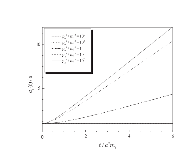
Figure 1: The time-dependence of the wave packet width $a_{\mbox{\tiny$i$}}\mbox{\footnotesize$(t)$}$ is given for different values of the ratio $p_{\mbox{\tiny$0$}}\,/\,m_{\mbox{\tiny$i$}}$. By considering a fixed mass value $m_{\mbox{\tiny$i$}}$, we compare the NR $(p_{\mbox{\tiny$0$}}\ll m_{\mbox{\tiny$i$}})$ and the UR $(p_{\mbox{\tiny$0$}}\gg m_{\mbox{\tiny$i$}})$ propagation regimes. We observe that the spreading is much more relevant in the former case. In the UR limit $(m_{\mbox{\tiny$i$}}=0)$, the wave packet does not spread and $a_{\mbox{\tiny$i$}}\mbox{\footnotesize$(t)$}$ assumes a constant value $a$.

The time-dependent quantities $a_{\mbox{\tiny$i$}}\mbox{\footnotesize$(t)$}$ and $\theta_{\mbox{\tiny$i$}}\mbox{\footnotesize$(t,z)$}$ contain all the physically significant informations which arise from the second-order term in the power series expansion (28). The spreading of the propagating wave packet can be immediately quantified by interpreting $a_{\mbox{\tiny$i$}}\mbox{\footnotesize$(t)$}$ as a time-dependent width, i. e., the spatial localization of the propagating particle is effectively given by $a_{\mbox{\tiny$i$}}\mbox{\footnotesize$(t)$}$ which increases during the time evolution. In the NR propagation regime, $a_{\mbox{\tiny$i$}}\mbox{\footnotesize$(t)$}$ reduces to $a^{\mbox{\tiny$NR$}}{\mbox{\tiny$i$}}\mbox{\footnotesize$(t)$}=a\sqrt{1+\frac{4}{a^{\mbox{\tiny$4$}}m_{s}^{\mbox{\tiny$2$}}}t^{\mbox{\tiny$2$}}}$ Coh77 . For times $t\gg a^{\mbox{\tiny$2$}}m_{\mbox{\tiny$i$}}$ the effective wave packet width $a^{\mbox{\tiny$NR$}}{\mbox{\tiny$i$}}\mbox{\footnotesize$(t)$}$ becomes much larger than the initial width $a$. On the other hand, the wave packet spreading in the UR propagation regime is approximated by $a^{\mbox{\tiny$UR$}}_{\mbox{\tiny$i$}}\mbox{\footnotesize$(t)$}=a\sqrt{1+\frac{4m_{s}^{\mbox{\tiny$4$}}}{a^{\mbox{\tiny$4$}}p_{o}^{\mbox{\tiny$6$}}}t^{\mbox{\tiny$2$}}}\approx a$. The UR spreading is practically negligible if we consider the same time-scale $T$ for both NR and UR cases, i. e., $a^{\mbox{\tiny$UR$}}_{\mbox{\tiny$i$}}\mbox{\footnotesize$(T)$}\ll a^{\mbox{\tiny$NR$}}_{\mbox{\tiny$i$}}\mbox{\footnotesize$(T)$}$. To illustrate this characteristic, we reproduce from Ber04 the time-dependence of $a_{\mbox{\tiny$i$}}\mbox{\footnotesize$(t)$}$ in Fig. 1 where we have assumed a particle with a definite mass value $m_{\mbox{\tiny$i$}}$. By computing the squared modulus of the mass-eigenstate wave function,

$$|\phi_{\mbox{\tiny$i$}}\mbox{\footnotesize$(z,t)$}|^{\mbox{\tiny$2$}}\approx\left(\frac{2}{\pi a^{\mbox{\tiny$2$}}_{\mbox{\tiny$i$}}\mbox{\footnotesize$(t)$}}\right)^{\frac{1}{2}}\exp{\left[-\frac{2(z-\mbox{v}_{\mbox{\tiny$i$}}\,t)^{\mbox{\tiny$2$}}}{a_{\mbox{\tiny$i$}}^{\mbox{\tiny$2$}}\mbox{\footnotesize$(t)$}}\right]},$$ (32)

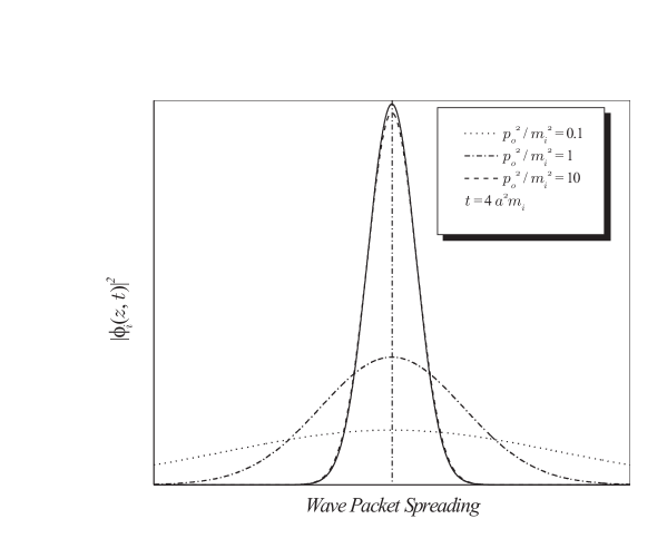
Figure 2: The wave packet spreading in both NR and UR propagation regimes is described at time $t=4a^{\mbox{\tiny$2$}}m_{\mbox{\tiny$i$}}$ in correspondence with Fig. 1. The solid line represent the shape of the wave packet at time $t=0$. In the case of an UR propagation expressed in terms of $\frac{p_{\mbox{\tiny$0$}}^{\mbox{\tiny$2$}}}{m_{\mbox{\tiny$i$}}^{\mbox{\tiny$2$}}}=10$, the spreading is indeed irrelevant.

we reproduce from Ber04 the wave packet spreading in both NR and UR propagation regimes in Fig. 2 which is in correspondence with Fig. 1. It confirms that the wave packet spreading is irrelevant for UR particles.

Returning to Eq. (29), we could interpret another second order effect by observing the time-behavior of the phase $\theta_{\mbox{\tiny$i$}}\mbox{\footnotesize$(t,z)$}$. By taking into account the wave packet localization, we assume that the amplitude of the wave function is relevant in the interval $|z-\mbox{v}_{\mbox{\tiny$i$}}\,t|\leq a_{\mbox{\tiny$i$}}\mbox{\footnotesize$(t)$}$. Due to the $z$-dependence, each wave packet space-point $z$ evolves in time in a different way. If we observe the propagation of the space-point $z=\mbox{v}_{\mbox{\tiny$i$}}\,t$, the increasing function $\theta_{\mbox{\tiny$i$}}\mbox{\footnotesize$(t,\,\mbox{v}_{\mbox{\tiny$i$}}t)$}$ assume values limited by the interval $[0,\frac{\pi}{4}[$. Otherwise, for any other space-point given by $z=\mbox{v}_{\mbox{\tiny$i$}}\,t+K\,a_{\mbox{\tiny$i$}}\mbox{\footnotesize$(t)$}$, $0<|K|\leq 1$, the phase $\theta_{\mbox{\tiny$i$}}\mbox{\footnotesize$(t,z)$}$ does not have a lower limit. We shall show in the next subsection that the presence of a time-dependent phase can modify the oscillation character of the flavor conversion formula. Anyway, the phase $\theta_{\mbox{\tiny$i$}}\mbox{\footnotesize$(t,z)$}$ is not influent on the free mass-eigenstate wave packet propagation as we can see from Eq. (32).

II.1.3 The oscillation probability

By evaluating the integral (13) with the approximation (28) and performing some mathematical manipulations, we obtain a factored expression for the interference term (9),

$$\mbox{\sc Int}\mbox{\footnotesize$(t)$}=\mbox{\sc Dmp}\mbox{\footnotesize$(t)$}\times\mbox{\sc Osc}\mbox{\footnotesize$(t)$},$$ (33)

which contains the damping term

$$\mbox{\sc Dmp}\mbox{\footnotesize$(t)$}=\left[1+\mbox{\sc Sp}^{\mbox{\tiny$2$}}\mbox{\footnotesize$(t)$}\right]^{-\frac{1}{4}}\exp{\left[-\frac{(\Delta\mbox{v}\,t)^{\mbox{\tiny$2$}}}{2a^{\mbox{\tiny$2$}}\left[1+\mbox{\sc Sp}^{\mbox{\tiny$2$}}\mbox{\footnotesize$(t)$}\right]}\right]}$$ (34)

and the oscillation term

Osc$$(t) = \mathrm{Re}\!\left\{\exp{\left[-i\Delta E\,t-i\Theta\mbox{\footnotesize$(t)$}\right]}\right\}$$ (35)

$$= \cos{\left[\Delta E\,t+\Theta\mbox{\footnotesize$(t)$}\right]},$$

where

$$\mbox{\sc Sp}\mbox{\footnotesize$(t)$}=\frac{t}{a^{\mbox{\tiny$2$}}}\Delta\left(\frac{m^{\mbox{\tiny$2$}}}{E^{\mbox{\tiny$3$}}}\right)=\rho\,\frac{\Delta\mbox{v}\,t}{a^{\mbox{\tiny$2$}}\,p_{\mbox{\tiny$0$}}}$$ (36)

and

$$\Theta\mbox{\footnotesize$(t)$}=\left[\mbox{\large$\frac{1}{2}$}\arctan{\left[\mbox{\sc Sp}\mbox{\footnotesize$(t)$}\right]}-\mbox{\large$\frac{a^{\mbox{\tiny$2$}}\,p_{\mbox{\tiny$0$}}^{\mbox{\tiny$2$}}}{2\rho^{\mbox{\tiny$2$}}}$}\frac{\mbox{\sc Sp}^{\mbox{\tiny$3$}}\mbox{\footnotesize$(t)$}}{\left[1+\mbox{\sc Sp}^{\mbox{\tiny$2$}}\mbox{\footnotesize$(t)$}\right]}\right],$$ (37)

with $\rho=1-\left[3+\left(\frac{\Delta E}{\bar{E}}\right)^{\mbox{\tiny$2$}}\right]\frac{p_{\mbox{\tiny$0$}}^{\mbox{\tiny$2$}}}{\bar{E}^{\mbox{\tiny$2$}}}$, $\Delta E=E_{\mbox{\tiny$1$}}-E_{\mbox{\tiny$2$}}$, $\bar{E}=\sqrt{E_{\mbox{\tiny$1$}}\,E_{\mbox{\tiny$2$}}}$ and $\Delta\mbox{v}=\mbox{v}_{1}-\mbox{v}_{2}$. The time-dependent quantities Sp$(t)$ and $\Theta\mbox{\footnotesize$(t)$}$ carry the second-order corrections and, consequently, the spreading effect to the oscillation probability formula. If $\Delta E\ll\bar{E}$, the parameter $\rho$ is limited by the interval $[1,-2]$ and it assumes the zero value when $\frac{p_{\mbox{\tiny$0$}}^{\mbox{\tiny$2$}}}{\bar{E}^{\mbox{\tiny$2$}}}\approx\frac{1}{3}$. Therefore, by considering increasing values of $p_{\mbox{\tiny$0$}}$, from NR (NR) to UR (UR) propagation regimes, and fixing $\frac{\Delta E}{a^{\mbox{\tiny$2$}}\,\bar{E}^{\mbox{\tiny$2$}}}$, the time derivatives of Sp$(t)$ and $\Theta\mbox{\footnotesize$(t)$}$ have their signals inverted when $\frac{p_{\mbox{\tiny$0$}}^{\mbox{\tiny$2$}}}{\bar{E}^{\mbox{\tiny$2$}}}$ reaches the value $\frac{1}{3}$.

The suppression of the oscillating behavior, which is primarily caused by the separation between the mass-eigenstate wave packets, is quantified by the damping term Dmp$(t)$. In order to compare Dmp$(t)$ with the correspondent function without the second-order corrections (without spreading),

$$\mbox{\sc Dmp}_{\mbox{\tiny$WS$}}\mbox{\footnotesize$(t)$}=\exp{\left[-\frac{(\Delta\mbox{v}\,t)^{\mbox{\tiny$2$}}}{2a^{\mbox{\tiny$2$}}}\right]},$$ (38)

we calculate the ratio between Eq. (34) and Eq. (38):

$$\frac{\mbox{\sc Dmp}\mbox{\footnotesize$(t)$}}{\mbox{\sc Dmp}_{\mbox{\tiny$WS$}}\mbox{\footnotesize$(t)$}} = \left[1+\rho^{\mbox{\tiny$2$}}\left(\frac{\Delta E\,t}{a^{\mbox{\tiny$2$}}\,\bar{E}^{\mbox{\tiny$2$}}}\right)^{\mbox{\tiny$2$}}\right]^{-\frac{1}{4}} \exp{\left[\frac{\rho^{\mbox{\tiny$2$}}\,p_{\mbox{\tiny$0$}}^{\mbox{\tiny$2$}}\,\left(\Delta E\,t\right)^{\mbox{\tiny$4$}}}{2\,a^{\mbox{\tiny$6$}}\,\bar{E}^{\mbox{\tiny$8$}}\left[1+\rho^{\mbox{\tiny$2$}}\left(\frac{\Delta E\,t}{a^{\mbox{\tiny$2$}}\,\bar{E}^{\mbox{\tiny$2$}}}\right)^{\mbox{\tiny$2$}}\right]}\right]}.$$ (39)

The NR limit is obtained by setting $\rho^{\mbox{\tiny$2$}}=1$ and $p_{\mbox{\tiny$0$}}=0$ in Eq. (38). In the same way, the UR limit is obtained by setting $\rho^{\mbox{\tiny$2$}}=4$ and $p_{\mbox{\tiny$0$}}=\bar{E}$. Between these limits, the minimal deviation from unity of Eq. (39) occurs when $\frac{p_{\mbox{\tiny$0$}}^{\mbox{\tiny$2$}}}{\bar{E}^{\mbox{\tiny$2$}}}\approx\frac{1}{3}$ ($\rho\approx 0$). Returning to the exponential term of Eq. (34), we observe that the oscillation amplitude is more relevant when $\Delta\mbox{v}\,t\ll a$. It characterizes the regime of minimal loss of coherence where the spatial overlap between the mass-eigenstate wave packets is significant. In such regime, we always have $\frac{\mbox{\sc Dmp}(t)}{\mbox{\sc Dmp}_{\mbox{\tiny$WS$}}(t)}\approx 1$.

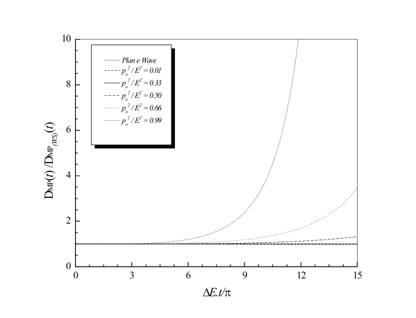
Figure 3: The comparison between the damping behavior with ($\mbox{\sc Dmp}(t)$) and without ($\mbox{\sc Dmp}_{\mbox{\tiny$WS$}}(t)$) the second order corrections for different propagation regimes. In order to have a realistic interpretation of the information carried by the second order corrections we arbitrarily fix $a\,\bar{E}=10$. The second order corrections could be indeed effective for both NR and (ultra)relativistic propagation regimes, however, the oscillations are destroyed much more rapidly in the latter case. If $\frac{p_{o}^{\mbox{\tiny$2$}}}{\bar{E}^{\mbox{\tiny$2$}}}\approx\frac{1}{3}$, the second order corrections are minimal.

We reproduce from Ber04 the Fig. 3 that shows the ratio of Eq. (39) for different propagation regimes, where we have arbitrarily set $a\,\bar{E}=10$. For asymptotic times, the time-dependent term $\mbox{\sc Sp}(t)$ effectively extends the interference between the mass-eigenstate wave packets since

$$\frac{\mbox{\sc Dmp}(t)}{\mbox{\sc Dmp}_{\mbox{\tiny$WS$}}(t)}\stackrel{{\scriptstyle t\rightarrow\infty}}{{\approx}}\frac{a\,\bar{E}}{(\rho\,\Delta E\,t)^{\frac{1}{2}}}\exp{\left[\frac{p_{o}^{\mbox{\tiny$2$}}\left(\Delta E\,t\right)^{\mbox{\tiny$2$}}}{2\,a^{\mbox{\tiny$2$}}\,\bar{E}^{\mbox{\tiny$4$}}}\right]}\gg 1,$$ (40)

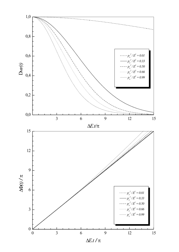
Figure 5: The behavior of the corrected phase $\Delta\Phi\mbox{\footnotesize$(t)$}=\Delta E\,t+\Theta\mbox{\footnotesize$(t)$}$ for different propagation regimes and we observe that the values assumed by $\Theta\mbox{\footnotesize$(t)$}$ are effective only when the interference boundary function Dmp$(t)$ does not vanish. By diminishing the value of the wave packet parameter $a\,\bar{E}$ (we have used $a\,\bar{E}=10$ for this plot) the amortizing behavior is attenuated and the range of modifications introduced by the additional phase $\Theta\mbox{\footnotesize$(t)$}$ increases.

but, in this case, the oscillations are almost completely destroyed by $\mbox{\sc Dmp}(t)$ (see Fig. 5).

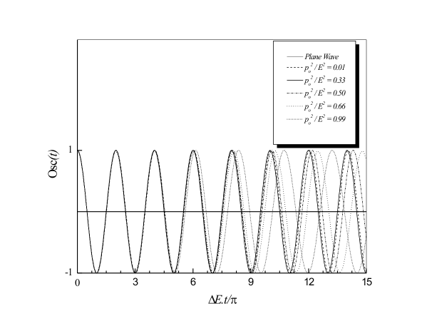
Figure 4: The time-behavior of Osc$(t)$ compared with the standard plane-wave oscillation given by $\cos{[\Delta E\,t]}$ for different propagation regimes. The additional phase $\Theta\mbox{\footnotesize$(t)$}$ changes the oscillating character after some time of propagation. The minimal deviation occurs for $\frac{p_{\mbox{\tiny$0$}}^{\mbox{\tiny$2$}}}{\bar{E}^{\mbox{\tiny$2$}}}\approx\frac{1}{3}$ which is represented by a solid line superposing the plane-wave case.

The oscillating function Osc$(t)$ of the interference term Int$(t)$ differs from the standard oscillating term, $\cos{[\Delta E\,t]}$, by the presence of the additional phase $\Theta\mbox{\footnotesize$(t)$}$ which is essentially a second-order correction. The modifications introduced by the additional phase $\Theta\mbox{\footnotesize$(t)$}$ are discussed in Fig. 4 where we have compared the time-behavior of Osc$(t)$ to $\cos{[\Delta E\,t]}$ for different propagation regimes. The effective bound value assumed by $\Theta\mbox{\footnotesize$(t)$}$ is determined by the damping behavior of Dmp$(t)$. To illustrate this flavor oscillation behavior, we plot both the curves representing Dmp$(t)$ and $\Theta\mbox{\footnotesize$(t)$}$ in Fig. 5. We note the phase changes slowly in the NR regime. The modulus of the phase $|\Theta\mbox{\footnotesize$(t)$}|$ rapidly reaches its upper limit when $\frac{p_{\mbox{\tiny$0$}}^{\mbox{\tiny$2$}}}{\bar{E}^{\mbox{\tiny$2$}}}>\frac{1}{3}$ and, after a certain time, it continues to evolve approximately linearly in time. Essentially, the oscillation vanishes rapidly. In case of (ultra-relativistic) neutrino oscillations, the values considered for $a$ in Figs. 4-5 are reproduced from Ber04 and they can be considered unrealistically large.

By superposing the effects of Dmp$(t)$ in Fig. 5 and the oscillating character Osc$(t)$ expressed in Fig. 4, we immediately obtain the flavor oscillation probability

$$\mathcal{P}(\bm{{\nu_{e}}}\rightarrow\bm{{\nu_{\mu}}};t)\approx\frac{\sin^{\mbox{\tiny$2$}}{(2\theta)}}{2}\left\{1-\left[1+\mbox{\sc Sp}^{\mbox{\tiny$2$}}\mbox{\footnotesize$(t)$}\right]^{-\frac{1}{4}}\exp{\left[-\frac{(\Delta\mbox{v}\,t)^{\mbox{\tiny$2$}}}{2a^{\mbox{\tiny$2$}}\left[1+\mbox{\sc Sp}^{\mbox{\tiny$2$}}\mbox{\footnotesize$(t)$}\right]}\right]}\cos{\left[\Delta E\,t+\Theta\mbox{\footnotesize$(t)$}\right]}\right\}\,,$$ (41)

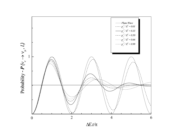
Figure 6: The time-dependence of the flavor conversion probability obtained with the introduction of second-order corrections in the series expansion of the energy for a strictly peaked momentum distribution ($\mathcal{O}(\sigma_{\mbox{\tiny$i$}}^{\mbox{\tiny$3$}})$). By comparing with the plane wave predictions, depending on the propagation regime, the additional time-dependent phase $\Delta\Phi\mbox{\footnotesize$(t)$}\equiv\,\Delta E\,t+\Theta\mbox{\footnotesize$(t)$}$ produces a delay/advance in the local maxima of flavor detection. Phenomenologically, we shall demonstrate that such modifications allow us to quantify small corrections to the averaged values of neutrino oscillation parameters, i. e., the mixing-angle and the mass-squared difference. Essentially, it depends on the product of the wave packet width $a$ by the averaged energy $\bar{E}$. Here again we have used $a\bar{E}=10$.

which is illustrated in Fig. 6.

Obviously, the larger is the value of $a\,\bar{E}$, the smaller are the wave packet effects. If it was sufficiently larger to not consider the second order corrections expressed in Eq. (28), we could compute the oscillation probability with the leading corrections due to the decoherence effect,

$$\mathcal{P}(\bm{{\nu_{e}}}\rightarrow\bm{{\nu_{\mu}}};t) \approx \frac{\sin^{\mbox{\tiny$2$}}{(2\theta)}}{2}\left\{1-\exp{\left[-\frac{(\Delta\mbox{v}\,t)^{\mbox{\tiny$2$}}}{2\,a^{\mbox{\tiny$2$}}}\right]}\cos{[\Delta E\,t]}\right\}$$ (42)

which corresponds to the same result obtained by DeL04 . Under minimal decoherence conditions ($\Delta\mbox{v}\,t\ll a$), the above expression reproduces the standard plane wave result,

$$\mathcal{P}(\bm{{\nu_{e}}}\rightarrow\bm{{\nu_{\mu}}};t) \approx \frac{\sin^{\mbox{\tiny$2$}}{(2\theta)}}{2}\left\{1-\cos{[\Delta E\,t]}\right\}=\sin^{\mbox{\tiny$2$}}(2\theta)\sin^{\mbox{\tiny$2$}}\left[\frac{\Delta m^{\mbox{\tiny$2$}}}{4\bar{E}}\,L\right]\,,$$ (43)

since we have assumed $a\,\bar{E}\gg 1$.

II.2 Initial flavor violation

The two family flavor conversion formula, obtained by simply associating scalar wave functions for neutrino mass-eigenstates, was given by Eq. (8). We can rewrite such expression, in the three-dimensional space, as

$$\mathcal{P}(\bm{{\nu_{e}}}\rightarrow\bm{{\nu_{\mu}}};t)=\frac{\sin^{\mbox{\tiny$2$}}{(2\theta)}}{4}\int d^{3}\!\bm{x}\,\big{|}\phi_{1}(\bm{x},t)-\phi_{2}(\bm{x},t)\big{|}^{2}\,.$$ (44)

It is evident from Eq. (44) that $\mathcal{P}(\bm{{\nu_{e}}}\rightarrow\bm{{\nu_{\mu}}};t)\neq 0$ if $\phi_{1}(\bm{x},t)\neq\phi_{2}(\bm{x},t)$ as complex functions of $\bm{x}$. In particular, for $t=0$, we necessarily have $\mathcal{P}(\bm{{\nu_{e}}}\rightarrow\bm{{\nu_{\mu}}};0)\neq 0$ if $\phi_{1}(\bm{x},0)\neq\phi_{2}(\bm{x},0)$. Therefore, we might have an initial flavor violation, without propagation, if the initial wave functions associated to the two neutrino mass-eigenstates are different. This leads to the problem of initial flavor definition in the formulation of neutrino oscillations DeL04 .

Three points of view can be adopted concerning initial flavor definition: (i) the ${\nu_{e}}\,$-flavor state is indeed well defined by Eq. (5) and we should have $\phi_{1}(\bm{x},0)=\phi_{2}(\bm{x},0)$ to guarantee (instantaneous) initial flavor definition; (ii) the definition of neutrino flavor should be generalized to accommodate more general initial conditions for neutrino creation; or (iii) exact flavor definition can not be achieved and initial flavor violation should be regarded as a genuine physical effect. Within the simple approach of intermediate scalar wave packets, we can only adopt the positions (i) and (ii), and only estimate the consequences of point of view (iii). We will see in the following that for a free and first quantized Dirac fermion the strict adoption of (i) leads to the inevitable presence of oscillating terms with short oscillation length $L^{VHF}_{Osc}=\frac{\pi}{p_{0}}=\frac{\Delta m^{2}}{4p^{2}_{0}}\,L^{Std}_{Osc}$, in addition to usual flavor oscillation characterized by the usual oscillation length $L^{Std}_{Osc}=\frac{4\pi p_{0}}{\Delta m^{2}}$. To avoid such rapid oscillations implies (iii), i. e., an initial non-null presence of the wrong flavor. Indeed, in the simple second quantized theory of Dirac fermion with mixing shown in section V.1 the adoption of (iii) is inevitable, although its consequence could be very small and unobservable in practice. Indeed, it is clear from the discussion after Eq. (12) that initial flavor violation effects implied by point of view (iii) should be small otherwise the amplitude of flavor oscillations would be highly suppressed. Moreover, large effects are excluded from neutrino conversion experiments. We can estimate the possible effects of flavor violation from Eq. (12), where gaussian wave packets were used. The probability of initial flavor violation is given by $\sin^{2}\!2\theta(a\Delta p/4)^{2}$, for $|a\Delta p|\ll 1$. Notice the condition $|a\Delta p|\ll 1$ is a particular version of the condition $\phi_{1}(\bm{x},t)\approx\phi_{2}(\bm{x},t)$ for gaussian wave packets of equal width.

To properly investigate (iii) and quantify its effects, it is necessary to go beyond the description of neutrino propagation and include the interactions responsible for neutrino creation (and detection). In terms of gaussian wave packets, it amounts to calculate the quantity $|a\Delta p|$ for realistic cases. Such task will be undertaken in section V.4 for neutrinos created in pion decay.

III Inclusion of spin and relativistic completeness

This section deals with the inclusion of spin and relativistic completeness in an relativistic quantum-mechanical derivation of the oscillation formula and some extensions. Neutrinos are fermions and we know that the time-evolution of a massive spin one-half particle has to be described by the Dirac equation. Firstly, we show how to include the spatial localization in the description of a flavor oscillating system when the dynamics of the Dirac equation is considered. In addition, we identify some common points between our results and some previous results for a quantum field approach for flavor oscillations Bla95 ; Giu02 ; Bla03 . Finally, we extend the discussion about initial flavor violation introduced in the previous section to the Dirac equation case. In particular, at the level of a quantum mechanical approach, we identify some relations between initial flavor violation and some predictable rapid oscillations.

It is well known that the Dirac equation, in its first quantized version, can give a significantly good description of a Dirac fermion if its inherent localization is much bigger than its Compton wave length; usually this is associated with weak external fields. For example, the spectrum for the hydrogen atom can be obtained with the relativistic corrections included (fine structure) Zub80 . One of the terms responsible for fine structure, the Darwin term, can be interpreted as coming from the interference between positive and negative frequency parts (zitterbewegung) of the hydrogen eigenfunction in Dirac theory compared to the NR theory FV ; Sak87 . On the other hand a situation where the theory fails to give a satisfactory physical description is exemplified by the Klein paradox Zub80 ; dombey:klein : the transmission coefficient for a electron moving towards a step barrier becomes negative for certain barrier heights, exactly when the localization of the electron wave function inside the barrier is comparable with its Compton wave length.

It is also well known that relativistic covariance requires the use of both positive and negative energy solutions for free relativistic particles. Otherwise, as we will see, functional completeness is lost, i. e., we can not expand a general solution of a relativistic wave equation in terms of only positive or negative eigenfunctions. Both types of solutions are also necessary to ensure relativistic causality, i. e., the time evolution of the solutions can not extend in space-time beyond the future lightcone of the initial spatial distribution.

Given the desirable properties of functional completeness and causality, which will be called relativistic completeness for short, we will treat in this section the flavor oscillation problem using the free Dirac theory in presence of two families mixing. We will see that the use of the Dirac equation will automatically encompass the properties of relativistic completeness.

Additionally, obtaining exact solutions of a generic class of Dirac wave equations Dir28 ; Esp99 ; Alh05 ; Ein81 ; Bak95 , specially with the presence of general interaction terms, is important because in some cases the conceptual understanding of the underlying physics can only be brought about by such solutions. These solutions also correspond to valuable means for checking and improving models and numerical methods for solving complicated physical problems. In the context in which we intend to explore the Dirac formalism, we can report about the Dirac wave packet treatment which can be useful in keeping clear many of the conceptual aspects of quantum oscillation phenomena that naturally arise in a relativistic spin one-half particle theory. In parallel, much progress on the theoretical front of the quantum mechanics of neutrino oscillations has been achieved, impelled by a phenomenological pursuit of a more refined flavor conversion formula Giu98 ; Zra98 ; Ber05 and by efforts to give the theory a formal structure within the quantum field formalism Bla95 ; Giu02 ; Bla03 .

To introduce the fermionic character in the study of quantum oscillation phenomena Ber05A ; Ber04 ; Ber05 ; ccn:no12 , we shall introduce the Dirac equation as the evolution equation for the mass-eigenstates. Hence, Eq. (5) becomes

$$\Psi\mbox{\footnotesize$(x)$} = \psi_{\mbox{\tiny$1$}}\mbox{\footnotesize$(x)$}\cos{\theta}\,\mbox{\boldmath$\nu_{\mbox{\tiny$1$}}$}+\psi_{\mbox{\tiny$2$}}\mbox{\footnotesize$(x)$}\sin{\theta}\,\mbox{\boldmath$\nu_{\mbox{\tiny$2$}}$}$$ (45)

$$= \left[\psi_{\mbox{\tiny$1$}}\mbox{\footnotesize$(x)$}\cos^{\mbox{\tiny$2$}}{\theta}+\psi_{\mbox{\tiny$2$}}\mbox{\footnotesize$(x)$}\sin^{\mbox{\tiny$2$}}{\theta}\right]\,\bm{{\nu_{e}}}+\left[\psi_{\mbox{\tiny$1$}}\mbox{\footnotesize$(x)$}-\psi_{\mbox{\tiny$2$}}\mbox{\footnotesize$(x)$}\right]\cos{\theta}\sin{\theta}\,\bm{{\nu_{\mu}}}$$

$$= \psi_{{\nu_{e}}}\mbox{\footnotesize$(x;\theta)$}\,\bm{{\nu_{e}}}+\psi_{{\nu_{\mu}}}\mbox{\footnotesize$(x;\theta)$}\,\bm{{\nu_{\mu}}}$$

where $x=(t,\bm{x})$ and $\psi_{\mbox{\tiny$i$}}\mbox{\footnotesize$(x)$}$, $i=1,2$, is a spinorial wave function, normalized to unity, that satisfies the Dirac equation for a mass $m_{\mbox{\tiny$i$}}$. The natural extension of Eq. (14) reads

$$\psi_{{\nu_{e}}}\mbox{\footnotesize$(\bm{x},\,t=0;\,\theta)$}\equiv\psi_{{\nu_{e}}}(\bm{x})=\psi_{1}\mbox{\footnotesize$(\bm{x},\,t=0)$}=\psi_{2}\mbox{\footnotesize$(\bm{x},\,t=0)$}\,,$$ (46)

which guarantees an initial pure flavor ${\nu_{e}}$. Therefore, the probability that an initial pure ${\nu_{e}}$ flavor be detected as ${\nu_{\mu}}$ flavor (8) is

$$\mathcal{P}(\mbox{\small$\bm{{\nu_{e}}}\!\rightarrow\!\bm{{\nu_{\mu}}}$};t)=\int\!d^{3}{x}\,\psi_{{\nu_{\mu}}}^{\dagger}\mbox{\footnotesize$(\bm{x},t)$}\psi_{{\nu_{\mu}}}\mbox{\footnotesize$(\bm{x},t)$}=\sin^{2}2\theta\frac{1}{2}\big{[}1-\mbox{\sc Dfo}\mbox{\footnotesize$(t)$}\big{]}\,,$$ (47)

where the interference term generalizing Eq. (9) for Dirac wave packets is

$$\mbox{\sc Dfo}\mbox{\footnotesize$(t)$}=\mathrm{Re}\int\!d^{3}{x}\,\psi_{1}^{\dagger}\mbox{\footnotesize$(\bm{x},\,t)$}\psi_{2}\mbox{\footnotesize$(\bm{x},\,t)$}\,.$$ (48)

More discussion on initial flavor definition within first quantized Dirac theory can be found in section III.5.

III.1 Dirac wave packets and the oscillation formula

Let us firstly consider the time evolution of a spin one-half free particle given by the Dirac equation

$$\left(i\gamma^{\mu}\partial_{\mu}-m\right)\psi\mbox{\footnotesize$(x)$}=0,$$ (49)

with the plane wave solutions given by $\psi\mbox{\footnotesize$(x)$}=\psi_{{}_{\mbox{\tiny$+$}}}\mbox{\footnotesize$(x)$}+\psi_{{}_{\mbox{\tiny$-$}}}\mbox{\footnotesize$(x)$}$ where

$$\psi_{{}_{\mbox{\tiny$+$}}}\mbox{\footnotesize$(x)$}=\exp{[-i\,p\,x]}\,u\mbox{\footnotesize$(p)$}~{}~{}~{}~{}\mbox{for positive frequencies and}$$

$$\psi_{{}_{\mbox{\tiny$-$}}}\mbox{\footnotesize$(x)$}=\exp{[+i\,p\,x]}\,v\mbox{\footnotesize$(p)$}~{}~{}~{}~{}\mbox{for negative frequencies};$$ (50)

$p$ is the relativistic quadrimomentum, $p=(E,\bm{p})$, and the relativistic energy is represented by $E=\sqrt{m^{\mbox{\tiny$2$}}+\bm{p}^{\mbox{\tiny$2$}}}$. The free propagating mass-eigenstate spinors are written as Pes95

$$u_{\mbox{\tiny$s$}}\mbox{\footnotesize$(p)$} = \frac{\gamma^{\mu}p_{\mu}+m}{\left[2\,E\,(m+E)\right]^{\frac{1}{2}}}\,u^{\mbox{\tiny$s$}}_{0}=\left(\begin{array}[]{r}\left(\frac{E+m}{2E}\right)^{\mbox{\tiny$\frac{1}{2}$}}\eta_{\mbox{\tiny$s$}}\raisebox{-7.20003pt}{}\\ \frac{\textstyle\bm{\Sigma}{\cdot}\bm{p}}{\left[2\,E\,(E+m)\right]^{\mbox{\tiny$\frac{1}{2}$}}}\eta_{\mbox{\tiny$s$}}\end{array}\right),$$ (53)

$$v_{\mbox{\tiny$s$}}\mbox{\footnotesize$(p)$} = \frac{-\gamma^{\mu}p_{\mu}+m}{\left[2\,E\,(m+E)\right]^{\mbox{\tiny$\frac{1}{2}$}}}\,\,v^{\mbox{\tiny$s$}}_{0}=\left(\begin{array}[]{r}\frac{\textstyle\bm{\Sigma}{\cdot}\bm{p}}{\left[2\,E\,(E+m)\right]^{\mbox{\tiny$\frac{1}{2}$}}}\eta_{\mbox{\tiny$s$}}\\ \raisebox{14.40007pt}{}\left(\frac{E+m}{2E}\right)^{\mbox{\tiny$\frac{1}{2}$}}\eta_{\mbox{\tiny$s$}}\end{array}\right),~{}~{}~{}$$ (56)

where $\eta_{\mbox{\tiny$1$},\mbox{\tiny$2$}}=\left(\begin{array}[]{c}1\\ 0\end{array}\right),\,\left(\begin{array}[]{c}0\\ 1\end{array}\right)$, $u^{\mbox{\tiny$s$}}_{0}\equiv u_{\mbox{\tiny$s$}}\mbox{\footnotesize$(m,\bm{0})$}$ $v^{\mbox{\tiny$s$}}_{0}\equiv v_{\mbox{\tiny$s$}}\mbox{\footnotesize$(m,\bm{0})$}$ are the spinors for zero momentum (they do not depend on the mass) and the relations $u_{s}^{\dagger}\mbox{\footnotesize$(p)$}u_{r}\mbox{\footnotesize$(p)$}=v_{s}^{\dagger}\mbox{\footnotesize$(p)$}v_{r}\mbox{\footnotesize$(p)$}=\delta_{rs}$ are satisfied. The right-hand sides of the second equalities of Eq. (56) assume the Dirac representation for the gamma matrices (see Eq. (143)). When more than one mass-eigenstate is in use, the positive and negative frequency eigenspinors will be respectively denoted by $u^{\mbox{\tiny$s$}}\mbox{\footnotesize$(\bm{p},m_{i})$}$ and $v^{\mbox{\tiny$s$}}\mbox{\footnotesize$(\bm{p},m_{i})$}$.

To describe the time evolution of mass-eigenstate Dirac wave packets, we could be inclined to superpose only positive frequency solutions of the Dirac equation. It seems, at first glance, a reasonable choice. However, for generic initial states it is usually necessary to superpose both positive and negative frequency solutions of the Dirac equation. We can show that both types of solution are necessary if we require the instantaneous creation of a pure $\bm{{\nu_{e}}}$ flavor, i.e., the mass-eigenstate wave functions satisfy $\psi_{\mbox{\tiny$1$}}(z,0)=\psi_{\mbox{\tiny$2$}}(z,0)$ in Eq. (46). (See sections II.2 and III.5.) More particularly, we can adopt the initial condition

$$\psi_{{\nu_{e}}}\mbox{\footnotesize$(\bm{x},\,t=0;\,\theta)$}=\phi_{{\nu_{e}}}\mbox{\footnotesize$(\bm{x})$}w\,,$$ (57)

obeying Eq. (46), where $\phi_{{\nu_{e}}}$ is a scalar wave function and $w$ is a constant spinor which satisfies the normalization condition $w^{\dagger}w=1$. That is not the most general condition because $w$ could depend on spatial coordinates, but it simplifies the preliminary calculations and allows a direct comparison to the scalar treatment of section II.

To continue the analysis, we turn back to the one-dimensional space ($\bm{x}\rightarrow z$) and express the flavor wave function $\psi_{{\nu_{e}}}(z,t,\theta)$ in terms of

$$\psi_{\mbox{\tiny$i$}}\mbox{\footnotesize$(z,t)$} = \int_{{}_{-\infty}}^{{}^{+\infty}}\!\frac{dp_{\mbox{\tiny$z$}}}{2\pi}\exp{[ip_{\mbox{\tiny$z$}}z]}\sum_{s=1,2}\{b^{s}\mbox{\footnotesize$(p_{\mbox{\tiny$z$}},m_{\mbox{\tiny$i$}})$}\,u^{s}\mbox{\footnotesize$(p_{\mbox{\tiny$z$}},m_{\mbox{\tiny$i$}})$}\exp{[-iE\mbox{\footnotesize$(p_{\mbox{\tiny$z$}},m_{\mbox{\tiny$i$}})$}t]}$$ (58)

$$\hskip 81.00014pt+\ d^{s*}\mbox{\footnotesize$(\mbox{\tiny$-$}p_{\mbox{\tiny$z$}},m_{\mbox{\tiny$i$}})$}\,v^{s}\mbox{\footnotesize$(\mbox{\tiny$-$}p_{\mbox{\tiny$z$}},m_{\mbox{\tiny$i$}})$}\exp{[+iE\mbox{\footnotesize$(p_{\mbox{\tiny$z$}},m_{\mbox{\tiny$i$}})$}t]}\}\,.$$

Therefore, since $\psi_{\mbox{\tiny$i$}}\mbox{\footnotesize$(z,0)$}=\psi_{{\nu_{e}}}\mbox{\footnotesize$(z,0,\theta)$}$ for $t=0$, the Fourier transform of Eq. (58) should be

$$\sum_{s=1,2}\left[b^{s}\mbox{\footnotesize$(p_{\mbox{\tiny$z$}},m_{\mbox{\tiny$i$}})$}\,u^{s}\mbox{\footnotesize$(p_{\mbox{\tiny$z$}},m_{\mbox{\tiny$i$}})$}+d^{s*}\mbox{\footnotesize$(\mbox{\tiny$-$}p_{\mbox{\tiny$z$}},m_{\mbox{\tiny$i$}})$}\,v^{s}\mbox{\footnotesize$(\mbox{\tiny$-$}p_{\mbox{\tiny$z$}},m_{\mbox{\tiny$i$}})$}\right] = \varphi\mbox{\footnotesize$(p_{\mbox{\tiny$z$}}-p_{\mbox{\tiny$0$}})$}w\,,\quad i=1,2\,,$$ (59)

where we used Eq. (57) and denoted $\varphi\mbox{\footnotesize$(p_{\mbox{\tiny$z$}}-p_{\mbox{\tiny$0$}})$}$ as the Fourier transform of $\phi_{{\nu_{e}}}\mbox{\footnotesize$(z)$}$. (In fact, the normalized Fourier transform of $\phi_{{\nu_{e}}}\mbox{\footnotesize$(z)$}$ is $\varphi\mbox{\footnotesize$(p_{\mbox{\tiny$z$}}-p_{\mbox{\tiny$0$}})$}/\sqrt{2\pi}$.) Using the orthogonality properties of Dirac spinors, we find Zub80

$$b^{s}\mbox{\footnotesize$(p_{\mbox{\tiny$z$}},m_{\mbox{\tiny$i$}})$} = \varphi\mbox{\footnotesize$(p_{\mbox{\tiny$z$}}-p_{\mbox{\tiny$0$}})$}\,u^{s\dagger}\mbox{\footnotesize$(p_{\mbox{\tiny$z$}},m_{\mbox{\tiny$i$}})$}\,w,$$

$$d^{s*}\mbox{\footnotesize$(\mbox{\tiny$-$}p_{\mbox{\tiny$z$}},m_{\mbox{\tiny$i$}})$} = \varphi\mbox{\footnotesize$(p_{\mbox{\tiny$z$}}-p_{\mbox{\tiny$0$}})$}\,v^{s\dagger}\mbox{\footnotesize$(\mbox{\tiny$-$}p_{\mbox{\tiny$z$}},m_{\mbox{\tiny$i$}})$}\,w.~{}~{}$$ (60)

These coefficients carry an important physical information. For any initial state which has the form given in Eq. (57), the negative frequency solution coefficient $d^{s*}\mbox{\footnotesize$(\mbox{\tiny$-$}p_{\mbox{\tiny$z$}},m_{\mbox{\tiny$i$}})$}$ necessarily provides a non-null contribution to the time evolving wave packet. This obliges us to take the complete set of Dirac equation solutions to construct the wave packet. In the general case, one can succeed to choose $\psi_{{\nu_{e}}}\mbox{\footnotesize$(z,0,\theta)$}$ in such a way that $\psi_{\mbox{\tiny$1$}}\mbox{\footnotesize$(z,0)$}=\psi_{{\nu_{e}}}\mbox{\footnotesize$(z,0,\theta)$}$ has vanishing coefficients $d^{s*}\mbox{\footnotesize$(\mbox{\tiny$-$}p_{\mbox{\tiny$z$}},m_{\mbox{\tiny$1$}})$}=0$ but then $\psi_{\mbox{\tiny$2$}}\mbox{\footnotesize$(z,0)$}=\psi_{{\nu_{e}}}\mbox{\footnotesize$(z,0,\theta)$}$ will necessarily contain non-vanishing coefficients $d^{s*}\mbox{\footnotesize$(\mbox{\tiny$-$}p_{\mbox{\tiny$z$}},m_{\mbox{\tiny$2$}})$}$ as it is shown in section III.5.

Having introduced the Dirac wave packet prescription, we are now in a position to calculate the flavor conversion formula. The following calculations do not depend on the gamma matrix representation. By substituting the coefficients given by Eq. (60) into Eq. (58) and using the well-known spinor properties Zub80 ,

$$\sum_{i=1,2}\mbox{$u^{s}\mbox{\footnotesize$(p_{\mbox{\tiny$z$}},m_{\mbox{\tiny$i$}})$}\overline{u}^{s}\mbox{\footnotesize$(p_{\mbox{\tiny$z$}},m_{\mbox{\tiny$i$}})$}$} = \frac{\gamma^{0}E\mbox{\footnotesize$(p_{\mbox{\tiny$z$}},m_{\mbox{\tiny$i$}})$}-\gamma^{\mbox{\tiny$3$}}p_{\mbox{\tiny$z$}}+m_{\mbox{\tiny$i$}}}{2E\mbox{\footnotesize$(p_{\mbox{\tiny$z$}},m_{\mbox{\tiny$i$}})$}},$$

$$\sum_{i=1,2}\mbox{$v^{s}\mbox{\footnotesize$(\mbox{\tiny$-$}p_{\mbox{\tiny$z$}},m_{\mbox{\tiny$i$}})$}\overline{v}^{s}\mbox{\footnotesize$(\mbox{\tiny$-$}p_{\mbox{\tiny$z$}},m_{\mbox{\tiny$i$}})$}$} = \frac{\gamma^{0}E\mbox{\footnotesize$(p_{\mbox{\tiny$z$}},m_{\mbox{\tiny$i$}})$}+\gamma^{\mbox{\tiny$3$}}p_{\mbox{\tiny$z$}}-m_{\mbox{\tiny$i$}}}{2E\mbox{\footnotesize$(p_{\mbox{\tiny$z$}},m_{\mbox{\tiny$i$}})$}},$$ (61)

we obtain

$$\psi_{\mbox{\tiny$i$}}\mbox{\footnotesize$(z,t)$}=\int_{{}_{-\infty}}^{{}^{+\infty}}\!\!\frac{dp_{\mbox{\tiny$z$}}}{2\pi}\,\varphi\mbox{\footnotesize$(p_{\mbox{\tiny$z$}}-p_{\mbox{\tiny$0$}})$}\exp{[ip_{\mbox{\tiny$z$}}z]}\left\{\cos{[E\mbox{\footnotesize$(p_{\mbox{\tiny$z$}},m_{\mbox{\tiny$i$}})$}t]}-\frac{i\gamma^{0}\left(\gamma^{\mbox{\tiny$3$}}p_{\mbox{\tiny$z$}}+m_{\mbox{\tiny$i$}}\right)}{E\mbox{\footnotesize$(p_{\mbox{\tiny$z$}},m_{\mbox{\tiny$i$}})$}}\sin{[E\mbox{\footnotesize$(p_{\mbox{\tiny$z$}},m_{\mbox{\tiny$i$}})$}t]}\right\}w\,.~{}~{}$$ (62)

By simple mathematical manipulations, the new interference oscillating term in Eq. (48) will be written as

Dfo$$(t) = \int_{{}_{-\infty}}^{{}^{+\infty}}\!\frac{dp_{\mbox{\tiny$z$}}}{2\pi}\,\varphi^{\mbox{\tiny$2$}}\mbox{\footnotesize$(p_{\mbox{\tiny$z$}}-p_{\mbox{\tiny$0$}})$}\left\{\left[1-f\mbox{\footnotesize$(p_{\mbox{\tiny$z$}},m_{\mbox{\tiny$1$},\mbox{\tiny$2$}})$}\right]\cos[\epsilon_{\mbox{\tiny$-$}}\mbox{\footnotesize$(p_{\mbox{\tiny$z$}},m_{\mbox{\tiny$1$},\mbox{\tiny$2$}})$}\,t]\right.$$ (64)

$$\hskip 81.00014pt\left.+\ f\mbox{\footnotesize$(p_{\mbox{\tiny$z$}},m_{\mbox{\tiny$1$},\mbox{\tiny$2$}})$}\cos[\epsilon_{\mbox{\tiny$+$}}\mbox{\footnotesize$(p_{\mbox{\tiny$z$}},m_{\mbox{\tiny$1$},\mbox{\tiny$2$}})$}\,t]\right\}$$

where

$$f\mbox{\footnotesize$(p_{\mbox{\tiny$z$}},m_{\mbox{\tiny$1$},\mbox{\tiny$2$}})$}=f\mbox{\footnotesize$(p_{\mbox{\tiny$z$}},m_{\mbox{\tiny$1$}},m_{\mbox{\tiny$2$}})$}=\frac{E\mbox{\footnotesize$(p_{\mbox{\tiny$z$}},m_{\mbox{\tiny$1$}})$}E\mbox{\footnotesize$(p_{\mbox{\tiny$z$}},m_{\mbox{\tiny$2$}})$}-p_{\mbox{\tiny$z$}}^{\mbox{\tiny$2$}}-m_{\mbox{\tiny$1$}}m_{\mbox{\tiny$2$}}}{2\,E\mbox{\footnotesize$(p_{\mbox{\tiny$z$}},m_{\mbox{\tiny$1$}})$}E\mbox{\footnotesize$(p_{\mbox{\tiny$z$}},m_{\mbox{\tiny$2$}})$}}$$

and

$$\epsilon_{\pm}\mbox{\footnotesize$(p_{\mbox{\tiny$z$}},m_{\mbox{\tiny$1$},\mbox{\tiny$2$}})$}=\epsilon_{\pm}\mbox{\footnotesize$(p_{\mbox{\tiny$z$}},m_{\mbox{\tiny$1$}},m_{\mbox{\tiny$2$}})$}=E\mbox{\footnotesize$(p_{\mbox{\tiny$z$}},m_{\mbox{\tiny$1$}})$}\pm E\mbox{\footnotesize$(p_{\mbox{\tiny$z$}},m_{\mbox{\tiny$2$}})$}~{}.$$

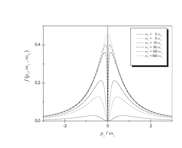
Figure 8: The function $f\mbox{\footnotesize$(p_{\mbox{\tiny$z$}},m{\mbox{\tiny$1$}},m_{\mbox{\tiny$2$}})$}$ is plotted for different values of the ratio between $m_{\mbox{\tiny$1$}}$ and $m_{\mbox{\tiny$2$}}$. For a momentum distribution sharply peaked around $p_{\mbox{\tiny$0$}}\gg m_{\mbox{\tiny$1$},\mbox{\tiny$2$}}$ (UR limit), $f\mbox{\footnotesize$(p_{\mbox{\tiny$z$}},m{\mbox{\tiny$1$}},m_{\mbox{\tiny$2$}})$}$ does not play a significant role in the “modified” oscillation formula. When the value of $m_{\mbox{\tiny$1$}}$ tends to the value of $m_{\mbox{\tiny$2$}}$, independently of the value of $p_{\mbox{\tiny$0$}}$ and of the width of the momentum distribution, the maximal value assumed by $f\mbox{\footnotesize$(p_{\mbox{\tiny$z$}},m{\mbox{\tiny$1$}},m_{\mbox{\tiny$2$}})$}$ tends to be negligible.

The time-independent term $f\mbox{\footnotesize$(p_{\mbox{\tiny$z$}},m_{\mbox{\tiny$1$}},m_{\mbox{\tiny$2$}})$}$ deserves some comments. It has a minimum at $p_{\mbox{\tiny$z$}}=0$ and two maxima at $p_{z}=\pm\sqrt{m_{\mbox{\tiny$1$}}m_{\mbox{\tiny$2$}}}$. We can readily observe in Fig. 8 that it goes rapidly to zero when $p_{\mbox{\tiny$z$}}\gg m_{1,2}$ (UR limit) as well as when $p_{\mbox{\tiny$0$}}\ll m_{1,2}$ (NR limit). It means that when we consider a momentum distribution sharply peaked around $p_{\mbox{\tiny$0$}}\gg m_{1,2}$ or $p_{\mbox{\tiny$0$}}\ll m_{1,2}$ the corrections introduced by $f\mbox{\footnotesize$(p_{\mbox{\tiny$z$}},m_{\mbox{\tiny$1$}},m_{\mbox{\tiny$2$}})$}$ are negligible. The maximum value of $f\mbox{\footnotesize$(p_{\mbox{\tiny$z$}},m_{\mbox{\tiny$1$}},m_{\mbox{\tiny$2$}})$}$ is

$$f_{max}=\frac{1}{2}-\frac{\sqrt{m_{\mbox{\tiny$1$}}m_{\mbox{\tiny$2$}}}}{m_{\mbox{\tiny$1$}}+m_{\mbox{\tiny$2$}}}=\frac{(\sqrt{m_{1}}-\sqrt{m_{2}})^{2}}{2(m_{1}+m_{2})}\,,$$ (65)

which vanishes in the limit $m_{\mbox{\tiny$1$}}=m_{\mbox{\tiny$2$}}$.

The effects introduced by $f\mbox{\footnotesize$(p_{\mbox{\tiny$z$}},m_{\mbox{\tiny$1$}},m_{\mbox{\tiny$2$}})$}$ are relevant only when $\Delta m\approx m_{\mbox{\tiny$1$}}\gg m_{\mbox{\tiny$2$}}$. Meanwhile, what is interesting about the result in Eq. (64) is that it was obtained without any assumption on the initial spinor $w$ or Fourier transform $\varphi\mbox{\footnotesize$(p_{\mbox{\tiny$z$}}-p_{\mbox{\tiny$0$}})$}$. Otherwise, the initial spinor carries some fundamental physical information about the created state. And this could be relevant in the study of chiral oscillations Ber06A ; Ber06B where the initial state plays a fundamental role. In comparison with the standard treatment of neutrino oscillations done by using scalar wave packets, where the interference term Int$(t)$ is given by Eq. (13) with $\Delta E(p_{\mbox{\tiny$z$}})\equiv\epsilon_{\mbox{\tiny$-$}}\mbox{\footnotesize$(p_{\mbox{\tiny$z$}},m_{\mbox{\tiny$1$}},m_{\mbox{\tiny$2$}})$}$, we notice in Dfo$(t)$ two additional terms. In the first one, the standard oscillating term $\cos{[\epsilon_{\mbox{\tiny$-$}}\mbox{\footnotesize$(p_{\mbox{\tiny$z$}},m_{\mbox{\tiny$1$},\mbox{\tiny$2$}})$}\,t]}$, which arises from the interference between mass-eigenstate components of equal sign frequencies, is multiplied by a new factor obtained by the products $u^{\dagger}\mbox{\footnotesize$(p_{\mbox{\tiny$z$}},m_{\mbox{\tiny$1$}})$}\,u\mbox{\footnotesize$(p_{\mbox{\tiny$z$}},m_{\mbox{\tiny$2$}})$}$, $v^{\dagger}(\mbox{\tiny$-$}p_{\mbox{\tiny$z$}},m_{\mbox{\tiny$1$}})\,v(\mbox{\tiny$-$}p_{\mbox{\tiny$z$}},m_{\mbox{\tiny$2$}})$ and h.c.. The second one is a new oscillating term, $\cos{[\epsilon_{\mbox{\tiny$+$}}\mbox{\footnotesize$(p_{\mbox{\tiny$z$}},m_{\mbox{\tiny$1$},\mbox{\tiny$2$}})$}\,t]}$, which comes from the interference between mass-eigenstate components of positive and negative frequencies. The factor multiplying such an additional oscillating term is obtained by the products $u^{\dagger}\mbox{\footnotesize$(p_{\mbox{\tiny$z$}},m_{\mbox{\tiny$1$}})$}\,v\mbox{\footnotesize$(\mbox{\tiny$-$}p_{\mbox{\tiny$z$}},m_{\mbox{\tiny$2$}})$}$, $v^{\dagger}\mbox{\footnotesize$(\mbox{\tiny$-$}p_{\mbox{\tiny$z$}},m_{\mbox{\tiny$1$}})$}\,u\mbox{\footnotesize$(p_{\mbox{\tiny$z$}},m_{\mbox{\tiny$2$}})$}$ and h.c..

The new oscillations have very high angular frequencies $\epsilon_{+}$. Indeed, we can find the relation $\epsilon_{+}\epsilon_{-}=\Delta m^{2}$, where $\epsilon_{-}$ is the usual (double of) flavor oscillation angular frequency. Such a peculiar oscillating behavior is similar to the phenomenon referred to as ZBW. In atomic physics, the electron exhibits this violent quantum fluctuation in the position and becomes sensitive to an effective potential which explains the Darwin term in the hydrogen atom Sak87 . We shall see later that, at the instant of creation, such rapid oscillations introduce a small modification in the oscillation formula.

III.2 The oscillation formula with first order corrections

A more satisfactory interpretation of the modifications introduced by the Dirac formalism is given when we explicitly calculate Dfo$(t)$. To that end, we resort to the same gaussian wave packet used in section II and use Eq. (14) for the scalar part $\phi_{{\nu_{e}}}\mbox{\footnotesize$(z)$}$ of the initial wave packet in Eq. (57):

$$\psi_{{\nu_{e}}}\mbox{\footnotesize$(z,\,t=0;\,\theta)$}=\phi_{{\nu_{e}}}(z)w=\left(\frac{2}{\pi a^{\mbox{\tiny$2$}}}\right)^{\frac{1}{4}}\exp{\left[-\frac{z^{\mbox{\tiny$2$}}}{a^{\mbox{\tiny$2$}}}\right]}\exp{[ip_{\mbox{\tiny$0$}}z]}\,w\,.$$ (66)

However, in contrast to section II, where we have considered the energy $E\mbox{\footnotesize$(p_{\mbox{\tiny$z$}},m_{\mbox{\tiny$i$}})$}$ expansion up to the second order terms in Eq. (28), so that the spreading effects were included in the analysis, we focus this preliminary study only on first order corrections. Thus, we approximate the frequency components by

$$E\mbox{\footnotesize$(p_{\mbox{\tiny$z$}},m_{\mbox{\tiny$i$}})$}\approx\,E_{\mbox{\tiny$i$}}\,+\mbox{v}_{\mbox{\tiny$i$}}\,\left(p_{\mbox{\tiny$z$}}-p_{\mbox{\tiny$0$}}\,\right)~{}.$$ (67)

Considering the approximation (67), we can write

$$f\mbox{\footnotesize$(p_{\mbox{\tiny$z$}},m_{\mbox{\tiny$1$}},m_{\mbox{\tiny$2$}})$}\approx\mbox{$\frac{1}{2}$}\,\left\{1-\mbox{v}_{\mbox{\tiny$1$}}\mbox{v}_{\mbox{\tiny$2$}}\left(1+\frac{m_{\mbox{\tiny$1$}}m_{\mbox{\tiny$2$}}}{p_{\mbox{\tiny$0$}}^{\mbox{\tiny$2$}}}\right)+\mbox{v}_{\mbox{\tiny$1$}}\mbox{v}_{\mbox{\tiny$2$}}\,\left[\left(\mbox{v}_{\mbox{\tiny$1$}}^{\mbox{\tiny$2$}}+\mbox{v}_{\mbox{\tiny$2$}}^{\mbox{\tiny$2$}}\right)\left(1+\frac{m_{\mbox{\tiny$1$}}m_{\mbox{\tiny$2$}}}{p_{\mbox{\tiny$0$}}^{\mbox{\tiny$2$}}}\right)-2\right]\,\frac{p_{\mbox{\tiny$z$}}-p_{\mbox{\tiny$0$}}}{p_{\mbox{\tiny$0$}}}\,\right\}$$ (68)

and

$$\epsilon_{\mbox{\tiny$\pm$}}\mbox{\footnotesize$(p_{\mbox{\tiny$z$}},m_{\mbox{\tiny$1$}},m_{\mbox{\tiny$2$}})$} \approx E_{\mbox{\tiny$1$}}\pm E_{\mbox{\tiny$2$}}+\left(\,\mbox{v}_{\mbox{\tiny$1$}}\pm\mbox{v}_{\mbox{\tiny$2$}}\,\right)\,\left(p_{\mbox{\tiny$z$}}-p_{\mbox{\tiny$0$}}\,\right)~{}.$$ (69)

For UR particles ($m_{\mbox{\tiny$i$}}\ll p_{\mbox{\tiny$0$}}$), we can also use the following expression for the central energy values ($E_{\mbox{\tiny$i$}}$) and the group velocities ($\mbox{v}_{\mbox{\tiny$i$}}$) of the mass-eigenstate wave packets,

$$E_{\mbox{\tiny$i$}}\approx\,p_{\mbox{\tiny$0$}}+\frac{m_{\mbox{\tiny$i$}}^{\mbox{\tiny$2$}}}{2\,p_{\mbox{\tiny$0$}}}~{}~{}~{}~{}~{}\mbox{and}~{}~{}~{}~{}~{}\mbox{v}_{\mbox{\tiny$i$}}\approx\,1-\frac{m_{\mbox{\tiny$i$}}^{\mbox{\tiny$2$}}}{2\,p_{\mbox{\tiny$0$}}^{\,\mbox{\tiny$2$}}}~{}.$$

This implies

$$f(p_{\mbox{\tiny$z$}},m_{\mbox{\tiny$1$}},m_{\mbox{\tiny$2$}}) \approx \left(\frac{\Delta m}{2\,p_{\mbox{\tiny$0$}}}\right)^{\mbox{\tiny$2$}}\,\left(\,1-2\,\,\frac{p_{\mbox{\tiny$z$}}-p_{\mbox{\tiny$0$}}}{p_{\mbox{\tiny$0$}}}\,\right)\,\,,$$

$$\epsilon_{\mbox{\tiny$+$}}\mbox{\footnotesize$(p_{\mbox{\tiny$z$}},m_{\mbox{\tiny$1$}},m_{\mbox{\tiny$2$}})$} \approx 2\,p_{\mbox{\tiny$0$}}\,\left[\,1\,+\,\frac{m_{\mbox{\tiny$1$}}^{\mbox{\tiny$2$}}+m_{\mbox{\tiny$2$}}^{\mbox{\tiny$2$}}}{4\,p_{\mbox{\tiny$0$}}^{\,\mbox{\tiny$2$}}}\,+\frac{p_{\mbox{\tiny$z$}}-p_{\mbox{\tiny$0$}}}{p_{\mbox{\tiny$0$}}}\,\left(\,1-\frac{m_{\mbox{\tiny$1$}}^{\mbox{\tiny$2$}}+m_{\mbox{\tiny$2$}}^{\mbox{\tiny$2$}}}{4\,p_{\mbox{\tiny$0$}}^{\,\mbox{\tiny$2$}}}\,\right)\,\right]\,\,,$$

$$\epsilon_{\mbox{\tiny$-$}}\mbox{\footnotesize$(p_{\mbox{\tiny$z$}},m_{\mbox{\tiny$1$}},m_{\mbox{\tiny$2$}})$} \approx \frac{\Delta m^{\mbox{\tiny$2$}}}{2\,p_{\mbox{\tiny$0$}}}\,\left[\,1-\,\frac{p_{\mbox{\tiny$z$}}-p_{\mbox{\tiny$0$}}}{p_{\mbox{\tiny$0$}}}\,\right]\,\,.$$

where $(\Delta m)^{\mbox{\tiny$2$}}=(m_{\mbox{\tiny$1$}}-m_{\mbox{\tiny$2$}})^{\mbox{\tiny$2$}}$ is different from $\Delta m^{\mbox{\tiny$2$}}=m_{\mbox{\tiny$1$}}^{\mbox{\tiny$2$}}-m_{\mbox{\tiny$2$}}^{\mbox{\tiny$2$}}$ which appears in the standard oscillation phase.

Finally, by simple algebraic manipulations and after gaussian integrations, we find for Eq. (64),

$$\mbox{\sc Dfo}\mbox{\footnotesize$(t)$}\approx\mbox{$\exp{\left[-\left(\frac{\Delta m^{\mbox{\tiny$2$}}\,t}{2\sqrt{2}ap_{\mbox{\tiny$0$}}^{\mbox{\tiny$2$}}}\right)^{\mbox{\tiny$2$}}\right]}\left\{\left[1-\left(\frac{\Delta m}{2p_{\mbox{\tiny$0$}}}\right)^{\mbox{\tiny$2$}}\right]\cos{\left[\frac{\Delta m^{\mbox{\tiny$2$}}}{2p_{\mbox{\tiny$0$}}}t\right]}+\left(\frac{\Delta m}{2p_{\mbox{\tiny$0$}}}\right)^{\mbox{\tiny$2$}}\frac{\Delta m^{\mbox{\tiny$2$}}}{a^{\mbox{\tiny$2$}}p_{\mbox{\tiny$0$}}^{\mbox{\tiny$3$}}}t\sin{\left[\frac{\Delta m^{\mbox{\tiny$2$}}}{2p_{\mbox{\tiny$0$}}}t\right]}\right\}$}$$ (70)

$$~{}~{}~{}~{}~{}~{}~{}~{}~{}~{}~{}~{}~{}~{}~{}~{}~{}~{}~{}~{}~{}~{}~{}~{}~{}~{}~{}~{}~{}~{}~{}~{}+\mbox{$\exp{\left[-\frac{t^{\mbox{\tiny$2$}}}{2a^{\mbox{\tiny$2$}}}\left(2-\frac{m_{\mbox{\tiny$1$}}^{\mbox{\tiny$2$}}+m_{\mbox{\tiny$2$}}^{\mbox{\tiny$2$}}}{2p_{\mbox{\tiny$0$}}^{\mbox{\tiny$2$}}}\right)^{\mbox{\tiny$2$}}\right]}\left(\frac{\Delta m}{2p_{\mbox{\tiny$0$}}}\right)^{\mbox{\tiny$2$}}\left\{\cos{\left[p_{\mbox{\tiny$0$}}t\left(2+\frac{m_{\mbox{\tiny$1$}}^{\mbox{\tiny$2$}}+m_{\mbox{\tiny$2$}}^{\mbox{\tiny$2$}}}{2p_{\mbox{\tiny$0$}}^{\mbox{\tiny$2$}}}\right)\right]}\right.$}$$

$$\mbox{$\left.~{}~{}~{}~{}~{}~{}~{}~{}~{}~{}~{}~{}~{}~{}~{}~{}~{}~{}~{}~{}~{}~{}~{}~{}~{}~{}~{}~{}~{}~{}~{}~{}~{}~{}~{}~{}~{}~{}~{}~{}~{}~{}~{}~{}~{}~{}~{}~{}~{}~{}~{}+\frac{2p_{\mbox{\tiny$0$}}t}{(ap_{\mbox{\tiny$0$}})^{\mbox{\tiny$2$}}}\left(2-\frac{m_{\mbox{\tiny$1$}}^{\mbox{\tiny$2$}}+m_{\mbox{\tiny$2$}}^{\mbox{\tiny$2$}}}{2p_{\mbox{\tiny$0$}}^{\mbox{\tiny$2$}}}\right)\sin{\left[p_{\mbox{\tiny$0$}}t\left(2+\frac{m_{\mbox{\tiny$1$}}^{\mbox{\tiny$2$}}+m_{\mbox{\tiny$2$}}^{\mbox{\tiny$2$}}}{2p_{\mbox{\tiny$0$}}^{\mbox{\tiny$2$}}}\right)\right]}\right\}$}.~{}~{}~{}~{}$$

As we have already noticed, the oscillating functions going with the second exponential function in Eq. (70) arise from the interference between positive and negative frequency solutions of the Dirac equation. It produces very high frequency oscillations which is similar to the quoted phenomenon of ZBW Sak87 . The oscillation length which characterizes the very high frequency oscillations is given by $L^{VHF}_{Osc}\approx\frac{\pi}{p_{\mbox{\tiny$0$}}}$. Obviously, $L^{VHF}_{Osc}$ is much smaller than the standard oscillation length given by $L^{Std}_{Osc}=\frac{4\pi p_{\mbox{\tiny$0$}}}{\Delta m^{\mbox{\tiny$2$}}}$. It means that the propagating particle exhibits a violent quantum fluctuation of its flavor quantum number around a flavor average value which oscillates with $L^{Std}_{Osc}$. Meanwhile, except at times $t\sim 0$, it provides a practically null contribution to the oscillation probability as we can observe in Fig. 7.

To explain such a statement, let us suppose that an experimental measurement takes place after a time $t\approx L$ for UR particles. The observability conditions impose that the propagation distance $L$ must be larger than the wave packet localization $a$. Since the (second) exponential function vanishes when $L\gg a$, for measurable distances, the effective flavor conversion formula will not contain such very high frequency oscillation terms, and can be written as

$$P_{\mbox{\tiny$Dirac$}}(\bm{{\nu_{e}}}\rightarrow\bm{{\nu_{\mu}}};L) \approx \frac{\sin^{\mbox{\tiny$2$}}{(2\theta)}}{2}\!\left\{1-\exp\!{\left[-\left(\!\frac{\Delta m^{\mbox{\tiny$2$}}\,L}{2\sqrt{2}ap_{\mbox{\tiny$0$}}^{\mbox{\tiny$2$}}}\right)^{\!\mbox{\tiny$2$}}\right]}\right.\!\left\{\left[1-\left(\!\frac{\Delta m}{2p_{\mbox{\tiny$0$}}}\!\right)^{\!\mbox{\tiny$2$}}\right]\!\cos\!{\left[\frac{\Delta m^{\mbox{\tiny$2$}}}{2p_{\mbox{\tiny$0$}}}L\right]}+~{}~{}\right.$$ (71)

$$~{}~{}~{}~{}~{}~{}~{}~{}~{}~{}~{}~{}~{}~{}~{}~{}~{}~{}~{}~{}~{}~{}~{}~{}~{}~{}~{}~{}~{}~{}~{}~{}~{}~{}~{}~{}~{}~{}~{}~{}~{}~{}~{}~{}~{}~{}~{}\left.\left.\left(\!\frac{\Delta m}{2p_{\mbox{\tiny$0$}}}\!\right)^{\!\mbox{\tiny$2$}}\!\frac{\Delta m^{\mbox{\tiny$2$}}}{a^{\mbox{\tiny$2$}}p_{\mbox{\tiny$0$}}^{\mbox{\tiny$3$}}}L\sin\!{\left[\frac{\Delta m^{\mbox{\tiny$2$}}}{2p_{\mbox{\tiny$0$}}}L\right]}\right\}\right\}\!.~{}~{}~{}$$

For distances which are restricted to the interval $a\ll L\ll a\frac{2\sqrt{2}p_{\mbox{\tiny$0$}}^{\mbox{\tiny$2$}}}{\Delta m^{\mbox{\tiny$2$}}}$, the interference term is preserved due to minimal slippage between the wave packets. In this case, we could approximate the oscillation probability to

$$P_{\mbox{\tiny$Dirac$}}(\bm{{\nu_{e}}}\rightarrow\bm{{\nu_{\mu}}};L) \approx \frac{\sin^{\mbox{\tiny$2$}}{(2\theta)}}{2}\left\{1-\left[1-\left(\frac{\Delta m^{\mbox{\tiny$2$}}L}{2\sqrt{2}ap_{\mbox{\tiny$0$}}^{\mbox{\tiny$2$}}}\right)^{\mbox{\tiny$2$}}\right]\left[1-\left(\frac{\Delta m}{2p_{\mbox{\tiny$0$}}}\right)^{\mbox{\tiny$2$}}\right]\cos{\left[\frac{\Delta m^{\mbox{\tiny$2$}}}{2p_{\mbox{\tiny$0$}}}L\right]}\right\}\,.$$ (72)

However, we reemphasize that it is not valid for $T\approx L\sim 0$ when the rapid oscillations are still relevant ($L<a$). By comparing the result of Eq. (72) with the scalar oscillation probability of Eq. (33), we notice a deviation of the order $\big{(}\!\frac{\Delta m}{2p_{\mbox{\tiny$0$}}}\!\big{)}^{\!\mbox{\tiny$2$}}$ that appears as an additional coefficient of the cosine function. It is not relevant in the UR limit as we have noticed after studying the function $f(p_{\mbox{\tiny$z$}},m_{\mbox{\tiny$1$}},m_{\mbox{\tiny$2$}})$.

III.3 Time evolution operator

An initial value problem, described by a differential equation, can be completely solved if we find a well defined kernel that governs the time evolution. Then from an initial field (wave function) configuration we can find the subsequent configurations at all subsequent times. Moreover, it is possible to analyze the properties of time evolution that are independent of the choice of the initial wave packet. Analyzing the properties of the kernel, it is also possible to check the properties of relativistic completeness for the free propagation of Dirac fermions with flavor mixing. Therefore, we will explicitly calculate, in this section, the time evolution operator (kernel) in presence of mixing in order to extract the common features independently of the initial wave packet. The extension to treat three families of neutrinos is straightforward. A matricial notation will be used throughout this subsection to express the mixing. Since the one-dimensional restriction does not lead to any formal simplification, the full three dimensional space will be considered here.

In matricial notation the mixing relation that extends Eq. (6), between flavor wave functions ${\Psi}_{f}^{\mathsf{T}}(\bm{x})\equiv(\psi_{\nu_{e}}^{\mathsf{T}}(\bm{x}),\psi_{\nu_{\mu}}^{\mathsf{T}}(\bm{x}))$ and mass wave functions ${\Psi}_{m}^{\mathsf{T}}(\bm{x})\equiv(\psi_{1}^{\mathsf{T}}(\bm{x}),\psi_{2}^{\mathsf{T}}(\bm{x}))$, is

$$\Psi_{f}(\bm{x})\equiv U\Psi_{m}(\bm{x})=\left(\begin{array}[]{cc}\phantom{\!\!\!-}\cos\!\theta&\sin\!\theta\cr\!\!\!-\sin\!\theta&\cos\!\theta\end{array}\right)\Psi_{m}(\bm{x})~{}.$$ (73)

Each mass wave function is defined as a four-component spinorial function $\psi_{n}(\bm{x},t)$, $n=1,2$ that satisfy the free Dirac equation (49)

$$i\frac{\partial}{\partial t}\psi_{n}(\bm{x},t)=H_{n}^{D}\psi_{n}(\bm{x},t)~{},~{}~{}n=1,2~{},$$ (74)

where the free Hamiltonian is the usual

$$H_{n}^{D}\equiv-i\bm{\alpha}{\cdot}\nabla+\beta m_{n}~{},~{}~{}n=1,2~{}.$$ (75)

The normalization condition is

$$\int d^{3}\!\bm{x}\,\Psi_{m}^{\dagger}(\bm{x})\Psi_{m}(\bm{x})=\int d^{3}\!\bm{x}\,\Psi_{f}^{\dagger}(\bm{x})\Psi_{f}(\bm{x})=1\,,$$ (76)

which implies that the wave functions $\psi_{1}(\bm{x})$ and $\psi_{2}(\bm{x})$, or, for the same reason, $\psi_{\nu_{e}}(\bm{x})$ and $\psi_{\nu_{\mu}}(\bm{x})$, can not be simultaneously normalized to unity. A different notation and normalization convention was being used through this review and it deserves a further clarification. As it can be seen in Eqs. (5) and (45), the wave functions for the mass-eigenstates were normalized to unity. To recover Eq. (45), the wave functions $\psi_{1}$ and $\psi_{2}$ used in this subsection, as in Eq. (73), should be replaced by

$$\psi_{1}\rightarrow\,\psi_{1}/\cos\theta\,,\qquad\psi_{2}\rightarrow\,\psi_{2}/\sin\theta\,.$$ (77)

This correspondence should be clear from the first line of Eq. (5). Equation (76) is a restatement of the fact that the probability to find a neutrino over all space irrespective of mass or irrespective of flavor is unity. We also see that condition (76) is time independent.

We will work in the flavor diagonal basis. This choice defines the flavor basis vectors simply as

$$\bm{\nu_{e}}\rightarrow\hat{\nu}_{e}=(1,0)^{\mathsf{T}}~{},~{}~{}\bm{\nu_{\mu}}\rightarrow\hat{\nu}_{\mu}=(0,1)^{\mathsf{T}}~{},$$ (78)

while the flavor projectors are obviously

$$\mathsf{P}_{\nu_{\alpha}}\equiv\hat{\nu}_{\alpha}\hat{\nu}_{\alpha}^{{\dagger}}\,.$$ (79)

Actually, as an abuse of notation, the equivalence $U\sim U\otimes\bm{1}_{D}$ is implicit, as well as, $\mathsf{P}_{\nu_{\alpha}}\sim\mathsf{P}_{\nu_{\alpha}}\otimes\bm{1}_{D}$; the symbol $\bm{1}_{D}$ refers to the identity matrix in spinorial space.

The total Hamiltonian governing the dynamics of $\Psi_{m}$ is $H^{D}=\mathrm{diag}(H_{1}^{D},H_{2}^{D})$. From the considerations above, $\Psi_{f}(\bm{x},t)$ satisfy the equation

$$i\frac{\partial}{\partial t}\Psi_{f}(\bm{x},t)\equiv UH^{D}U^{-1}\Psi_{f}(\bm{x},t)~{}.$$ (80)

The solution to the equation above can be written in terms of a flavor evolution operator $K^{D}$ as

$$\Psi_{f}(\bm{x},t)=K^{D}(t)\Psi_{f}(\bm{x},0)=\int\!d^{3}{\bm{x}^{\prime}}\,K^{D}(\bm{x}-\bm{x}^{\mbox{\tiny$\prime$}};t)\Psi_{f}(\bm{x}^{\mbox{\tiny$\prime$}},0)~{},$$ (81)

where

$$K^{D}(\bm{x}-\bm{x}^{\mbox{\tiny$\prime$}};t)=\int\!\frac{d^{3}\!\bm{p}}{(2\pi)^{3}}\,K^{D}(\bm{p};t)\,e^{i\bm{p}\cdot(\bm{x}-\bm{x}^{\mbox{\tiny$\prime$}})}~{}.$$ (82)

We can calculate $K^{D}(t)$ in any representation (momentum or position) as

$$K^{D}(t) = Ue^{-iH^{D}t}U^{-1}$$ (83)

$$= \left(\begin{array}[]{cc}\cos^{2}\!\theta\,e^{-iH_{1}^{D}t}+\sin^{2}\!\theta\,e^{-iH_{2}^{D}t}&-\cos\!\theta\sin\!\theta(e^{-iH_{1}^{D}t}-e^{-iH_{2}^{D}t})\cr-\cos\!\theta\sin\!\theta(e^{-iH_{1}^{D}t}-e^{-iH_{2}^{D}t})&\sin^{2}\!\theta\,e^{-iH_{1}^{D}t}+\cos^{2}\!\theta\,e^{-iH_{2}^{D}t}\end{array}\right)~{}.$$ (86)

It is important to emphasize that Eq. (81) leads to a causal propagation because the kernel in Eq. (82) respects $K^{D}(\bm{x}-\bm{x}^{\mbox{\tiny$\prime$}};t)=0$ for space-like distances $|\bm{x}-\bm{x}^{\prime}|>|t|$. This property follows directly from Eq. (83) and the properties of causality of each kernel, $\langle\bm{x}|e^{-iH_{n}^{D}t}|\bm{x}^{\prime}\rangle=0$ for $|\bm{x}-\bm{x}^{\prime}|>|t|$, associated to the Dirac Hamiltonian with mass $m_{n}$, $n=1,2$ [see Eqs. (293) and (361) or Ref. thaller ].

The conversion probability is then

$$\mathcal{P}(\mbox{\small$\bm{\nu_{e}}\!\rightarrow\!\bm{\nu_{\mu}}$};t) = \int\!d^{3}{\bm{x}}\,\Psi_{f}^{{\dagger}}(\bm{x},0)K^{D\,{\dagger}}(t)\mathsf{P}_{\nu_{\mu}}K^{D}(t)\Psi_{f}(\bm{x},0)$$ (87)

$$= \int\!d^{3}{\bm{p}}\,\tilde{\psi}_{\nu_{e}}^{{\dagger}}(\bm{p})(K_{\mu e}^{D})^{\dagger}K_{\mu e}^{D}(\bm{p},t)\tilde{\psi}_{\nu_{e}}(\bm{p})~{},$$ (88)

satisfying the initial condition $\Psi_{f}^{\mathsf{T}}(\bm{x},0)=(\psi^{\mathsf{T}}_{\nu_{e}}(\bm{x},0),0)$. Such initial condition implies, in terms of mass eigenfunctions, $\psi_{1}(\bm{x},0)=\cos\theta\,\psi_{\nu_{e}}(\bm{x})$ and $\psi_{2}(\bm{x},0)=\sin\theta\,\psi_{\nu_{e}}(\bm{x})$, as a requirement to obtain an initial wave function with definite flavor, as seen in section II.2 DeL04 . The function $\tilde{\psi}_{\nu_{e}}(\bm{p})$ denotes the inverse Fourier transform of $\psi_{\nu_{e}}(\bm{x})$ (see Eqs. (344) and (345)).

Before obtaining the conversion probability for Dirac fermions, let us replace the spinorial functions $\psi_{n}(\bm{x})$ by spinless one-component wave functions $\varphi_{n}(\bm{x})$ in the flavor wave function ${\Psi}_{f}^{\mathsf{T}}(\bm{x})\rightarrow(\varphi_{\nu_{e}}(\bm{x}),\varphi_{\nu_{\mu}}(\bm{x}))$ and mass wave function ${\Psi}_{m}^{\mathsf{T}}(\bm{x})\rightarrow(\varphi_{1}(\bm{x}),\varphi_{2}(\bm{x}))$. We also replace the Dirac Hamiltonian in momentum space $H^{D}_{n}(\bm{p})$ (75) by the relativistic energy $E_{n}(\bm{p})=\sqrt{\bm{p}^{2}+m^{2}_{n}}$. Inserting these replacements into Eq. (87) we can recover the usual oscillation probability DeL04 ; Ber05

$$\mathcal{P}(\mbox{\small$\bm{\nu_{e}}\!\rightarrow\!\bm{\nu_{\mu}}$};t) = \int\!d^{3}{\bm{x}}\,|\hat{\nu}_{\mu}^{\mathsf{T}}\Psi_{f}(\bm{x},t)|^{2}$$ (89)

$$= \int\!d^{3}{\bm{p}}\,|K^{S}_{\mu e}(\bm{p},t)\tilde{\varphi}_{\nu_{e}}(\bm{p})|^{2}$$ (90)

$$= \int\!d^{3}{\bm{p}}\,\mathscr{P}(\bm{p},t)|\tilde{\varphi}_{\nu_{e}}(\bm{p})|^{2}~{},$$ (91)

where $\Psi_{f}(\bm{x},0)^{\mathsf{T}}=(\varphi_{\nu_{e}}(\bm{x})^{\mathsf{T}},0)$, $K^{S}_{\mu e}(\bm{p},t)\equiv(K^{S})_{21}=-\sin\theta\cos\theta(e^{-iE_{1}(\bm{p})t}-e^{-iE_{2}(\bm{p})t})$ and

$$\mathscr{P}(\bm{p},t)=\sin^{2}\!2\theta\sin^{2}\!(\Delta E\mbox{\footnotesize$(\bm{p})$}t/2)~{}$$ (92)

is just the standard oscillation formula (1) with $\Delta E\mbox{\footnotesize$(\bm{p})$}\equiv E_{1}\mbox{\footnotesize$(\bm{p})$}-E_{2}\mbox{\footnotesize$(\bm{p})$}$. The conversion probability (89) in this case is then the standard oscillation probability smeared out by the initial momentum distribution. If the substitution $|\tilde{\varphi}_{\nu_{e}}(\bm{p})|^{2}\rightarrow\delta^{3}(\bm{p}-\bm{p}_{0})$ is made the standard oscillation formula is recovered: it corresponds to the plane-wave limit.

After we have checked the standard oscillation formula can be recovered for spinless particles restricted to positive energies, we can return to the case of Dirac fermions. We can obtain explicitly the terms of the mixed evolution kernel (83) by using the property of the Dirac Hamiltonian in momentum space $(H_{n}^{D})^{2}=E_{n}^{2}(\bm{p})\,\bm{1}_{D}$, which leads to

$$(K_{\mu e}^{D})^{\dagger}K_{\mu e}^{D}(\bm{p},t) = \mathscr{P}(\bm{p},t)[1-f(\bm{p})]\bm{1}_{D}$$ (94)

$$+\,\sin^{2}\!2\theta f(\bm{p})\sin^{2}(\bar{E}\mbox{\footnotesize$(\bm{p})$}\,t)\bm{1}_{D}~{},$$

where

$$f(\bm{p})=\frac{1}{2}[1-\frac{\bm{p}^{2}+m_{1}m_{2}}{E_{1}E_{2}}]~{},$$ (95)

$\bar{E}\mbox{\footnotesize$(\bm{p})$}\equiv\frac{1}{2}[E_{1}\mbox{\footnotesize$(\mathbf{p})$}+E_{1}\mbox{\footnotesize$(\mathbf{p})$}]$ endnote0 and $\mathscr{P}(\bm{p},t)$ is the standard conversion probability function (92). The expression (95) was already found in Eq. (64) in a slightly different form. A unique implication of Eq. (94), which is proportional to the identity matrix in spinorial space, is that the conversion probability (87) does not depend on the spinorial structure of the initial flavor wave function but only on its momentum density as

$$\mathcal{P}(\mbox{\small$\bm{\nu_{e}}\!\rightarrow\!\bm{\nu_{\mu}}$};t)=\int\!d^{3}{\bm{p}}\,\{\mathscr{P}(\bm{p},t)[1-f(\bm{p})]\hskip 30.00005pt$$

$$+~{}\sin^{2}\!2\theta f(\bm{p})\sin^{2}(\bar{E}t)\}\,\tilde{\psi}^{\dagger}_{\nu_{e}}(\bm{p})\tilde{\psi}_{\nu_{e}}(\bm{p})\,.$$ (96)

(The tilde will denote the inverse Fourier transformed function throughout this subsection.) Furthermore, the modifications in Eq. (III.3) compared to the scalar conversion probability (89) are exactly the same modifications found in Eq. (64) if we replace $\varphi^{\mbox{\tiny$2$}}\mbox{\footnotesize$(p_{\mbox{\tiny$z$}}-p_{\mbox{\tiny$0$}})$}/2\pi$ by $\tilde{\psi}^{\dagger}_{\nu_{e}}(\bm{p})\tilde{\psi}_{\nu_{e}}(\bm{p})$ and use three-dimensional integration.

The conservation of total probability

$$\mathcal{P}(\mbox{\small$\bm{{\nu_{e}}}\!\rightarrow\!\bm{{\nu_{\mu}}}$};t)+\mathcal{P}(\mbox{\small$\bm{{\nu_{e}}}\!\rightarrow\!\bm{{\nu_{e}}}$};t)=1~{},$$ (97)

is automatic in virtue of

$$K_{ee}^{D{\dagger}}(\bm{p},t)K_{ee}^{D}(\bm{p},t)+K_{\mu e}^{D{\dagger}}(\bm{p},t)K_{\mu e}^{D}(\bm{p},t)=\bm{1}_{D}~{},$$ (98)

and initial normalization in Eq. (76). The survival and conversion probability for an initial muon neutrino are identical to the probabilities for an initial electron neutrino because of the relations

$$K_{\mu\mu}^{D{\dagger}}(\bm{p},t)K_{\mu\mu}^{D}(\bm{p},t) = K_{ee}^{D{\dagger}}(\bm{p},t)K_{ee}^{D}(\bm{p},t)~{},$$ (99)

$$K_{\mu e}^{D{\dagger}}(\bm{p},t)K_{\mu e}^{D}(\bm{p},t) = K_{e\mu}^{D{\dagger}}(\bm{p},t)K_{e\mu}^{D}(\bm{p},t)~{}.$$ (100)

III.4 Spinless neutrinos

The derivation of the usual conversion probability (89) takes into account only the positive frequency contributions. The mass wave function used to obtain Eq. (89) corresponds to the solutions of the wave equation

$$i\frac{\partial}{\partial t}\varphi(\bm{x},t)=\sqrt{-\nabla^{2}+m^{2}}\,\varphi(\bm{x},t)~{},$$ (101)

which is equivalent to the Dirac equation in the Foldy-Wouthuysen representation FW , restricted to positive energies. The evolution kernel for this equation is not satisfactory from the point of view of causality thaller , i.e, the kernel is not null for spacelike intervals. Moreover, the eigenfunctions restricted to one sign of energy do not form a complete set FV .

To recover a causal propagation in the spin 0 case, the Klein-Gordon wave equation must be considered. In the first quantized version, the spectrum of the solutions have positive and negative energy as in the Dirac case. However, to take advantage of the Hamiltonian formalism used in section III.3, it is more convenient do work in the Sakata-Taketani (ST) Hamiltonian formalism FV where each mass wave function is formed by two components

$$\Phi_{n}(\bm{x},t)=\left(\begin{array}[]{c}\varphi_{n}(\bm{x},t)\cr\chi_{n}(\bm{x},t)\end{array}\right)~{},~{}~{}n=1,2\,.$$ (102)

The components $\varphi$ and $\chi$ are combinations of the usual scalar Klein-Gordon wave function $\phi(x)$ and its time derivative $\partial_{0}\phi(x)$. This is necessary since the Klein-Gordon equation is a second order differential equation in time and the knowledge of the function and its time derivative is necessary to completely define the time evolution. An analysis of the flavor oscillation of scalar wave functions obeying the Klein-Gordon equation can be found in Ref. dvornikov .

The time evolution in this formalism is governed by the Hamiltonian FV

$$H_{n}^{\mbox{\tiny$ST$}}=-(\tau_{3}+i\tau_{2})\frac{\nabla^{2}}{2m_{n}}+m_{n}^{2}~{},$$ (103)

which satisfies the condition $(H_{n}^{\mbox{\tiny$ST$}})^{2}=(-\nabla^{2}+m_{n}^{2})\bm{1}_{\mbox{\tiny$ST$}}$, like the Dirac Hamiltonian (75). The $\tau_{k}$ represents the usual Pauli matrices and $\bm{1}_{\mbox{\tiny$ST$}}$ is the identity matrix.

A charge density endnote1 can be defined as

$$\bar{\Phi}_{n}\Phi_{n}\equiv\Phi_{n}^{\dagger}\tau_{3}\Phi_{n}=|\varphi_{n}|^{2}-|\chi_{n}|^{2}~{},$$ (104)

which is equivalent to the one found in Klein-Gordon notation $i\phi^{*}\overset{\leftrightarrow}{\partial}_{0}\phi$. Needless to say, this density (104) is only non-null for complex (charged) wave functions. The charge density $\bar{\Phi}\Phi$ is the equivalent of fermion probability density $\psi^{{\dagger}}\psi$ in the Dirac case, although the former is not positive definite as the latter. The adjoint $\bar{\Phi}=\Phi^{\dagger}\tau_{3}$ were defined to make explicit the (non positive definite) norm structure of the conserved charge

$$\int\!d^{3}{\bm{x}}\,\bar{\Phi}_{n}(\bm{x},t)\Phi_{n}(\bm{x},t)\equiv(\Phi_{n},\Phi_{n})=\text{time independent}~{}.$$ (105)

Consequently, the adjoint of any operator $\Omega$ can be defined as $\bar{\Omega}=\tau_{3}\Omega^{\dagger}\tau_{3}$, satisfying $(\bar{\Omega}\Phi,\Phi)=(\Phi,\Omega\Phi)$. Within this notation, the Hamiltonians of Eq. (103) is self-adjoint, $\bar{H}_{n}^{\mbox{\tiny$ST$}}=H_{n}^{\mbox{\tiny$ST$}}$, and the time invariance of Eq. (105) is assured.

We can assemble, as in the previous section, the mass wave functions into $\Psi_{m}^{\mathsf{T}}\equiv(\Phi_{1}^{\mathsf{T}},\Phi_{2}^{\mathsf{T}})$ and the flavor wave functions into $\Psi_{f}^{\mathsf{T}}\equiv(\Phi_{\nu_{e}}^{\mathsf{T}},\Phi_{\nu_{\mu}}^{\mathsf{T}})$, satisfying the mixing relation $\Psi_{f}\equiv U\Psi_{m}$. Then, the time evolution of $\Psi_{f}$ can be given through a time evolution operator $K^{\mbox{\tiny$ST$}}$ acting in the same form as in Eq. (81). In complete analogy to the calculations from Eq. (82) to Eq. (87), we can define the conversion probability as

$$\mathcal{P}(\mbox{\small$\bm{\nu_{e}}\!\rightarrow\!\bm{\nu_{\mu}}$};t) = \int\!d^{3}{\bm{x}}\,\bar{\Psi}_{f}(\bm{x},0)\overline{K^{\mbox{\tiny$ST$}}(t)}\mathsf{P}_{\nu_{\mu}}K^{\mbox{\tiny$ST$}}(t)\Psi_{f}(\bm{x},0)$$ (106)

$$= \int\!d^{3}{\bm{p}}\,\overline{\tilde{\Phi}_{e}(\bm{p})}\overline{K_{\mu e}^{\mbox{\tiny$ST$}}}K_{\mu e}^{\mbox{\tiny$ST$}}(\bm{p},t)\tilde{\Phi}_{e}(\bm{p})~{},$$ (107)

where $\Psi_{f}(\bm{x},0)^{\mathsf{T}}=(\Phi_{e}(\bm{x})^{\mathsf{T}},0)$. The adjoint operation were also extended to $\bar{\Psi}_{f}=\Psi_{f}^{\dagger}(\bm{1}_{\theta}\otimes\tau_{3})$, where $\bm{1}_{\theta}$ is the identity in mixing space.

The information of time evolution, hence oscillation, is all encoded in

$$\overline{K_{\mu e}^{\mbox{\tiny$ST$}}}K_{\mu e}^{\mbox{\tiny$ST$}}(\bm{p},t) = \mathscr{P}(\bm{p},t)[1-f(\mu\bm{p})]\bm{1}_{\mbox{\tiny$ST$}}$$ (109)

$$+~{}\sin^{2}\!2\theta f(\mu\bm{p})\sin^{2}(\bar{E}t)\bm{1}_{\mbox{\tiny$ST$}}~{},$$

where the function $f(\bm{p})$ were already defined in Eq. (95) and

$$\mu=\sqrt{\frac{1}{2}(\frac{m_{1}}{m_{2}}+\frac{m_{2}}{m_{1}})}~{}.$$ (110)

The factor $\mu\geq 1$ determines the difference with the Dirac case in Eq. (94). The equality $\mu=1$ holds when $m_{1}=m_{2}$, i. e., when there is no oscillation.

Therefore, rapid oscillations are also present in flavor oscillations of charged (in the sense of Eq. (104)) spin 0 particles, with contributions slightly different from the Dirac case. Such result reinforces the fact that rapid oscillations are direct consequences of flavor mixing, (a) relativistic nature of the wave equations governing time evolution and (b) initial flavor definition. The presence of a spinorial degree of freedom is not a requirement to rapid oscillations.

III.5 Initial flavor violation and rapid oscillations

We saw in Eqs. (64) and (III.3) that the flavor conversion probability for Dirac fermions presents rapid oscillation terms with frequency $2\bar{E}=E_{1}(\bm{p})+E_{2}(\bm{p})$, in addition to the usual oscillation frequency $\Delta E=E_{1}(\bm{p})-E_{2}(\bm{p})=\frac{m^{2}_{1}-m^{2}_{2}}{E_{1}(\bm{p})+E_{2}(\bm{p})}$. Such frequencies arise naturally from the propagation of free particles with mixing in a relativistic classical field theory that contains states with positive and negative frequencies $\pm E_{i}(\bm{p})$, e.g., spin 1/2 fermions and spin 0 bosons. It was assumed, however, that flavor can be well defined and a pure ${\nu_{e}}$ flavor is created at $t=0$. We will elucidate here that such rapid oscillations can be avoided but only at the expense of not having an initial flavor exactly defined. More specifically, we will see there is a clash between two choices:

• cond. A: exact initial flavor definition (pure flavor creation) and

• cond. B: standard flavor oscillation, without rapid oscillations.

Firstly, following the formalism of subsection III.3, we calculate the probability that a generic superposition of neutrinos $\nu_{1}$ and $\nu_{2}$, denoted simply by $\nu$, described by a generic $\Psi_{m}$, be detected as a neutrino ${\nu_{\mu}}$:

$$\mathcal{P}(\bm{\nu}\!\rightarrow\!\bm{{\nu_{\mu}}};t)=\int d\bm{x}\,\Psi_{m}^{\dagger}(\bm{x})e^{-iH^{D}t}\mathsf{P}_{\nu_{\mu}}e^{-iH^{D}t}\Psi_{m}(\bm{x})\,,$$ (111)

where the operator inside, in the mass-basis, can be calculated explicitly

$$e^{-iH^{D}t}\mathsf{P}_{\nu_{\mu}}e^{-iH^{D}t}=\begin{pmatrix}\sin^{2}\theta&-\sin\theta\cos\theta e^{iH_{1}^{D}t}e^{-iH_{2}^{D}t}\cr-\sin\theta\cos\theta e^{iH_{2}^{D}t}e^{-iH_{1}^{D}t}&\cos^{2}\theta\end{pmatrix}\,.$$ (112)

Notice in this section we are working in the mass-basis, keeping the same notation as in section III.3, where $(\mathsf{P}_{\nu_{\mu}})_{ij}=\hat{\nu}_{\mu}\hat{\nu}_{\mu}^{\dagger}=U^{*}_{\mu i}U_{\mu j}$, since $(\hat{\nu}_{\alpha})_{i}\equiv U^{*}_{\alpha i}$ and $(\hat{\nu}_{i})=\delta_{ij}$ in this basis. Only the off-diagonal terms depend on time $t$, and energies $E_{1}$ and $E_{2}$, which means the functional dependence on time and energies, in momentum space, should be of the form $g(\Delta Et,\bar{E}t)$, where $\Delta E\equiv\,E_{1}(\bm{p})-E_{2}(\bm{p})$ and $2\bar{E}\equiv E_{1}(\bm{p})+E_{2}(\bm{p})$. Such functional form is in accordance to Eq. (III.3), for example. To disentangle the dependencies on $\Delta Et$ and $\bar{E}t$, it is instructive to rewrite the free Dirac time evolution operator, in momentum space, in the form

$$e^{-iH_{n}^{D}t}=e^{-iE_{n}t}\Lambda_{n+}^{D}+e^{iE_{n}t}\Lambda_{n-}^{D}~{},$$ (113)

where

$$\Lambda_{n\pm}^{D}=\frac{1}{2}(\bm{1}_{D}\pm\frac{H_{n}^{D}}{E_{n}})~{},$$ (114)

are the projector operators to positive (+) or negative (-) energy eigenstates of $H_{n}^{D}$. By using the decomposition above (113), we can separate the different contributions in the off-diagonal terms of Eq. (112) by rewriting

$$e^{iH_{1}^{D}t}e^{-iH_{2}^{D}t} = e^{i\Delta Et}\Lambda_{1+}^{D}\Lambda_{2+}^{D}+e^{-i\Delta Et}\Lambda_{1-}^{D}\Lambda_{2-}^{D}$$ (116)

$$+~{}e^{i2\bar{E}t}\Lambda_{1+}^{D}\Lambda_{2-}^{D}+e^{-i2\bar{E}t}\Lambda_{1-}^{D}\Lambda_{2+}^{D}\,.~{}~{}~{}$$

The same procedure can be applied to its hermitian conjugate. The time evolution kernel of Eq. (83), in the flavor basis, can be analyzed in the same fashion. Since $\Lambda_{1\pm}^{D}\Lambda_{2\mp}^{D}\neq 0$, it can be seen that the rapid oscillating terms come from the interference between, e. g., the positive frequencies of the Hamiltonian $H_{1}^{D}$ and negative frequencies of the Hamiltonian $H_{2}^{D}$.

We know that both positive and negative energy states should propagate properly to preserve causality. With a kernel containing only positive energy contributions $e^{-iE_{n}t}$, there is no causal propagation thaller . Therefore, to maintain causality, we can not eliminate, for example, the negative energy contribution in the kernel of Eq. (113). One may, of course, restrict the initial wave functions to contain only positive energy states. Such restriction eliminates the rapid oscillatory terms, also known as zitterbewegung, for a one-particle free Dirac theory Zub80 . For two masses, however, the positive energy eigenfunctions with respect to a basis characterized by a mass $m_{1}$ necessarily have non-null components of negative energy with respect to another basis characterized by $m_{2}$, as we will see.

Let us examine exact initial flavor definition (cond. A). Firstly, we introduce wave functions $\psi_{1}$ and $\psi_{2}$, normalized to unity, by using

$$\Psi_{m}=\begin{pmatrix}\cos\alpha\,\psi_{1}\cr\sin\alpha\,\psi_{2}\end{pmatrix}\,,~{}~{}0\leq\alpha\leq\frac{\pi}{2}\,;$$ (117)

where additional phases can be easily incorporated in $\psi_{1},\psi_{2}$. Then Eq. (111) yields

$$\mathcal{P}(\bm{\nu}\!\rightarrow\!\bm{{\nu_{\mu}}};t)=\sin^{2}(\theta+\alpha)\sin^{2}(\mbox{\normalsize$\frac{1}{2}$}\Xi_{t})+\sin^{2}(\theta-\alpha)\cos^{2}(\mbox{\normalsize$\frac{1}{2}$}\Xi_{t})\,,$$ (118)

where we used the following parametrization for Eq. (48),

$$\cos\Xi_{t}=\mathrm{Re}\int\!d^{3}\!\bm{x}\,\psi_{1}^{\dagger}(\bm{x},t)\psi_{2}(\bm{x},t)\,,~{}~{}0\leq\Xi_{t}\leq\pi\,,$$ (119)

which is consistent with $|\cos\Xi_{t}|\leq 1$ for normalized $\psi_{1}$ and $\psi_{2}$. Obviously $\psi_{i}(\bm{x},t)=e^{-iH_{i}^{D}t}\psi_{i}(\bm{x})$. Since the expression in Eq. (118) is a sum of non-negative terms, to have $\mathcal{P}(\mbox{\small$\bm{\nu}\!\rightarrow\!\bm{{\nu_{\mu}}}$};0)=0$ at $t=0$, we should have

$$\theta-\alpha=0\,,~{}~{}\text{ and }~{}~{}\Xi_{0}=0\,.$$ (120)

The other possibilities, $\theta+\alpha=0$ or $\theta+\alpha=\pi$, are outside the parameter range of $\alpha$ since $0<\theta<\pi/2$ for non-trivial mixing. Moreover, $\alpha=\theta$ corresponds to the only local and global minimum of the second term of Eq. (118) as a function of $\alpha$. The function $\sin^{2}(\alpha+\theta)$ in the first term of Eq. (118) is always non-null and has the global minimum at the borders $\alpha=0$ or $\alpha=\pi/2$. The second equality in Eq. (120) is equivalent to

$$\psi_{1}(\bm{x},0)=\psi_{2}(\bm{x},0)=\psi(\bm{x})\,.$$ (121)

Thus the necessary and sufficient initial conditions for initial pure ${\nu_{e}}$ flavor or, equivalently (for two flavors), no ${\nu_{\mu}}$ flavor, restricts Eq. (117) to

$$\Psi_{m}(\bm{x})=\begin{pmatrix}U^{*}_{e1}\psi_{1}(\bm{x})\cr U^{*}_{e2}\psi_{2}(\bm{x})\end{pmatrix}=U^{*}_{ei}\psi_{i}(\bm{x})\hat{\nu}_{i}=\psi(\bm{x})\hat{\nu}_{e}\,,$$ (122)

where in the last equality, Eq. (121) was explicitly assumed. Although condition (121) can be also inferred from Eq. (87), restricted to Eq. (76), we showed an alternative derivation without assuming a fixed proportion between mass-eigenstates, which is a more general initial condition than the one used in section II.2.

Let us now try to eliminate rapid oscillations (cond. B) by adjusting the initial conditions. This was not attempted so far. We begin by considering only positive energy states for

$$\psi_{i}(\bm{x})=\psi_{i}^{(+)}(\bm{x})~{},~{}~{}i=1,2\,,$$ (123)

in Eq. (117). In momentum space, Eq. (123) can be written

$$\tilde{\psi}_{i}^{(+)}(\bm{p})=\sum_{s}u^{s}(\bm{p},m_{i})g_{i}(\bm{p},s)\,,$$ (124)

where the spinors $u^{s}$ were defined in Eq. (56). By construction, $\Lambda_{i+}\psi_{i}^{(+)}(\bm{x})=\psi_{i}^{(+)}(\bm{x})$ and $\Lambda_{i-}\psi_{i}^{(+)}(\bm{x})=0$, which means $\psi_{i}(\bm{x},t)=e^{-iH_{i}^{D}t}\psi_{i}(\bm{x})$ only contains the positive energy term $e^{-iE_{i}(\bm{p})t}$ in its Fourier transform. In this case, the time dependent function $\Xi_{t}$ in the ${\nu_{\mu}}$ detection probability (118) is given by

$$\cos\Xi_{t} = \mathrm{Re}\!\int\!d^{3}\!\bm{p}\,\tilde{\psi}_{1}^{\dagger}(\bm{p})\tilde{\psi}_{2}(\bm{p})e^{i\Delta E(\bm{p})t}$$ (125)

$$= \mathrm{Re}\sum_{s}\!\int\!d^{3}\!\bm{p}\,g_{1}^{*}(\bm{p},s)g_{2}(\bm{p},s)e^{i\Delta E(\bm{p})t}[1-2f_{2}(\bm{p})]\,,$$ (126)

where

$$f_{2}(\bm{p})\equiv\frac{1}{2}-\frac{1}{4}\sqrt{1+x_{1}}\sqrt{1+x_{2}}-\frac{1}{4}\sqrt{1-x_{1}}\sqrt{1-x_{2}}\,,$$ (127)

defined with the shorthand $x_{i}\equiv\frac{m_{i}}{E_{i}(\bm{p})}$. We used the calculation

$$u^{r{\dagger}}(\bm{p},m_{\mbox{\tiny$1$}})u^{s}(\bm{p},m_{\mbox{\tiny$2$}})=[1-2f_{2}(\bm{p})]\,\delta_{rs}\,.$$ (128)

We achieved our goal: there is no rapid oscillations. The probability $\mathcal{P}(\bm{\nu}\!\rightarrow\!\bm{{\nu_{\mu}}};t)$ is only a function of $\Delta E(\bm{p})t$ smeared out in momentum.

Let us now show that restriction (120) for cond. A can not be simultaneously applied with restriction (123) for cond. B.

Let us suppose cond. A [Eq. (121)] is valid, i. e., $\psi_{1}(\bm{x})=\psi_{2}(\bm{x})=\psi(\bm{x})$. We can decompose the spinorial function $\psi(\bm{x})$ in terms of bases depending on different masses $m_{1}$ and $m_{2}$. Equating

$$\psi(\bm{x})=\int\!\frac{d^{3}\!\bm{p}}{\sqrt{2E_{i}}}\,[u_{i}^{s}(\bm{x};\bm{p})g_{i}^{\mbox{\tiny$(+)$}}(\bm{p},s)+v_{i}^{s}(\bm{x};\bm{p})g_{i}^{\mbox{\tiny$(-)$}}(\bm{p},s)]~{},~{}~{}i=1,2\,,$$ (129)

where $\mbox{\large$\frac{u_{i}^{s}(\bm{x};\bm{p})}{\sqrt{2E_{i}}}$}\equiv u^{s}\mbox{\footnotesize$(\bm{p},m_{i})$}\,\mbox{\small$e^{i\bm{p}\,{\cdot}\bm{x}}/(2\pi)^{\mbox{\tiny$3/2$}}$}$ and $\mbox{\large$\frac{v_{i}^{s}(\bm{x};\bm{p})}{\sqrt{2E_{i}}}$}\equiv v^{s}\mbox{\footnotesize$(\bm{p},m_{i})$}\,\mbox{\small$e^{-i\bm{p}\,{\cdot}\bm{x}}/(2\pi)^{\mbox{\tiny$3/2$}}$}$, the expansion coefficients can be obtained

$$g_{i}^{\mbox{\tiny$(+)$}}(\bm{p},s) = \int\!d^{3}\!\bm{x}\,\mbox{\large$\frac{u_{i}^{s{\dagger}}\!(\bm{x};\bm{p})}{\sqrt{2E_{i}}}$}\psi(\bm{x})~{},$$ (130)

$$g_{i}^{\mbox{\tiny$(-)$}}(\bm{p},s) = \int\!d^{3}\!\bm{x}\,\mbox{\large$\frac{v_{i}^{s{\dagger}}\!(\bm{x};\bm{p})}{\sqrt{2E_{i}}}$}\psi(\bm{x})~{}.$$ (131)

From Eq. (131), and $\tilde{\psi}(\bm{p})$ being the inverse Fourier transform of $\psi(\bm{x})$, we see that imposing the conditions

$$g_{1}^{\mbox{\tiny$(-)$}}(\bm{p},s) = v^{s{\dagger}}\mbox{\footnotesize$(\bm{p},m_{\mbox{\tiny$1$}})$}\tilde{\psi}(-\bm{p})=0~{},$$ (132)

$$g_{2}^{\mbox{\tiny$(-)$}}(\bm{p},s) = v^{s{\dagger}}\mbox{\footnotesize$(\bm{p},m_{\mbox{\tiny$2$}})$}\tilde{\psi}(-\bm{p})=0~{},$$ (133)

for all $\bm{p}$, leads to the conditions

$$\mbox{\small$[(m_{1}+E_{2})-(m_{2}+E_{2})]$}\,v_{0}^{s{\dagger}}\tilde{\psi}(-\bm{p}) = 0~{},~{}s=1,2\,,$$ (134)

$$\mbox{\large$\Big{[}\frac{1}{m_{1}+E_{2}}-\frac{1}{m_{2}+E_{2}}\Big{]}$}\,v_{0}^{s{\dagger}}\bm{\gamma}.\bm{p}\,\tilde{\psi}(-\bm{p}) = 0~{},~{}s=1,2\,,$$ (135)

where the property of Eq. (353) and $\gamma_{0}v_{0}^{s}=-v_{0}^{s}$ were used. In case $m_{1}\neq m_{2}$, we can use the decomposition $\tilde{\psi}(\bm{p})=\tilde{\psi}_{+}(\bm{p})+\tilde{\psi}_{-}(\bm{p})$, where $\tilde{\psi}_{\pm}(\bm{p})=(\bm{1}\pm\gamma_{0})\tilde{\psi}(\bm{p})$/2, and obtain from Eqs. (134) and (135) the conditions

$$v_{0}^{s{\dagger}}\tilde{\psi}_{-}(-\bm{p}) = 0~{},~{}s=1,2\,,$$ (136)

$$u_{0}^{s{\dagger}}\bm{\Sigma}{\cdot}\bm{p}\,\tilde{\psi}_{+}(-\bm{p}) = 0~{},~{}s=1,2\,,$$ (137)

where the properties $\bm{\gamma}=\gamma_{0}\gamma_{5}\bm{\Sigma}$ and $u_{0}^{s}=\gamma_{5}v_{0}^{s}$ were used in Eq. (137). Since $\bm{\Sigma}{\cdot}\bm{p}$ has only non-null eigenvalues and it commutes with $\gamma_{0}$, the equations (136) and (137) are only satisfied if $\tilde{\psi}_{+}(\bm{p})=\tilde{\psi}_{-}(\bm{p})=0$, i. e., $\psi(\bm{x})=0$. It is easier to reach this conclusion in the helicity basis $\{u_{0}^{\mbox{\tiny$(\pm)$}},v_{0}^{\mbox{\tiny$(\pm)$}}\}$ characterized by $\bm{\Sigma}{\cdot}\bm{p}\,u_{0}^{\mbox{\tiny$(\pm)$}}=\pm|\bm{p}|u_{0}^{\mbox{\tiny$(\pm)$}}$, but the result is basis independent.

We can then conclude that rapid oscillations are an inevitable consequence of a relativistic Dirac fermion description of flavor oscillations if initial flavor definition is exactly required. Quantitatively, however, it was seen in Eqs. (64) and (94) that the contribution of rapid oscillations to the probability $\mathcal{P}(\mbox{\small$\bm{{\nu_{e}}}\!\rightarrow\!\bm{{\nu_{\mu}}}$};t)$ is negligible for momentum distributions around UR values because rapid oscillation is quantified by the function $f$ in Eq.  (95), which behaves as $f\sim(\Delta m)^{2}/(4\bar{E}^{2})$ for UR momenta. On the other hand, it was already shown that avoiding rapid oscillations is possible to the detriment of having initial flavor violation.

Let us quantify the amount of initial flavor violation for neutrinos states of the form (123) satisfying cond. B. Let us relax the conditions of Eq. (120), and consider only the first one, $\alpha=\theta$, which is a minimum in $\alpha$. Thus the initial probability to detect the wrong flavor ${\nu_{\mu}}$ can be rewritten by using Eq. (126) as

$$\frac{\mathcal{P}(\mbox{\small$\bm{{\nu_{e}}}\!\rightarrow\!\bm{{\nu_{\mu}}}$};0)}{\sin^{2}2\theta} = \frac{1}{4}\sum_{s}\int\!d^{3}\!\bm{p}\,\Big{\{}|g_{1}(\bm{p},s)-g_{2}(\bm{p},s)|^{2}+4f_{2}(\bm{p})\mathrm{Re}\big{[}g_{1}^{*}(\bm{p},s)g_{2}(\bm{p},s)\big{]}\Big{\}},~{}~{}~{}~{}$$ (138)

where we used the expansion (124).

We immediately see that taking equal momentum distributions for the two mass-eigenstates (for two spin states), i. e.,

$$g_{1}(\bm{p},s)=g_{2}(\bm{p},s)=g(\bm{p},s)\,,$$ (139)

makes the first term of Eq. (138) vanish. Initial flavor violation is then proportional to

$$\frac{\mathcal{P}(\mbox{\small$\bm{{\nu_{e}}}\!\rightarrow\!\bm{{\nu_{\mu}}}$};0)}{\sin^{2}2\theta} = \int\!d^{3}\!\bm{p}\,|g(\bm{p})|^{2}f_{2}(\bm{p})\,,$$ (140)

where $|g(\bm{p})|^{2}=\sum_{s}|g(\bm{p},s)|^{2}$ is the spin-independent momentum distribution. Notice the normalization

$$\int\!d^{3}\!\bm{p}\,|g(\bm{p})|^{2}=1\,.$$ (141)

As it should be, $f_{2}(\bm{p})=0$ if $m_{1}=m_{2}$ and it behaves as $f_{2}\sim(\Delta m)^{2}/(4\bar{E})^{2}$ for UR momenta. Moreover, $f_{2}(\bm{p})$ has the unique maximum value at $|\bm{p}|=\sqrt{m_{1}m_{2}}$, the same point as $f(\bm{p})$. In fact, the function $f_{2}$ and the function $f(\bm{p})$ in Eq. (95) are closely related by the relation

$$[1-2f_{2}(\bm{p})]^{2}=1-f(\bm{p})\,.$$ (142)

Therefore initial flavor violation in Eq. (140) is also negligible for momentum distributions around UR momenta, provided that Eq. (139) is valid.

We can conclude that the description of flavor oscillations for a free Dirac fermion subjected to mixing, within first quantization, is satisfactory from the quantitative point of view but in the strict sense one should consider either one of the following phenomena as inevitably present: (i) initial flavor violation or (ii) rapid oscillations. Both effects might be as negligible as Eqs. (140) or (94) (or Eq. (64)), quantified by the functions $f_{2}(\bm{p})$ or $f(\bm{p})$, respectively. We will see (i) is supported by second quantization. In that case, it is possible that such effect could be still small but larger than Eq. (140). All depends on how different are $\psi_{1}(\bm{x})$ and $\psi_{2}(\bm{x})$, associated to the two mass-eigenstates, when a neutrino is created as a superposition of mass-eigenstates. Furthermore, the presence of (i) suggests that neutrino flavor is not an exact concept but only an approximately well defined one.

IV Consequences of spin structure and relativistic completeness

This section deals with some intrinsic consequences of spin structure and relativistic completeness, namely chiral oscillations and the consequences for a non-minimal coupling with external magnetic fields. Chiral oscillations naturally enter the discussion of neutrino oscillations since neutrinos are produced and detected through weak interactions that are chiral in nature. We succeed in showing that the inclusion of chiral oscillation effects, together with the time-evolution of spinorial wave packets for the mass-eigenstates, can modify the flavor conversion probability formula. In particular, it provides an interpretation of chiral oscillations as very rapid oscillations in position along the direction of motion, i.e., longitudinal to the momentum of the particle. All the ingredients for decoupling chiral oscillations from the spin-flipping in the presence of an external magnetic field are discriminated. It allows for depicting all the relevant effects due to the inclusion of spin structure and relativistic completeness that we have introduced.

According to the SM at tree level, neutrinos interact with itself and other leptons only through weak charged current and neutral current interactions which are chiral in nature and only contain the contribution of neutrinos with negative chirality DeL98 . Consequently, positive chirality neutrinos become sterile with respect to V-A weak charged currents, independently of any external electromagnetic field. Despite the experimental circumstances not being favorable to such an interpretation, the quantum transitions that produces a final flavor state corresponding to an active-sterile quantum mixing is perfectly acceptable from the theoretical point of view. Even focusing specifically on the chiral oscillation mechanism, we have also observed a generic interest in identifying the physical meaning of variables which coexist with the interference between positive and negative frequency solutions of Dirac equation Bra99 ; Rup00 ; Wan01 ; Bol04 in a Dirac wave packet treatment. If we follow an almost identical line of reasoning as that applied for rapid oscillations of the position, it is also possible to verify that the average value of the Dirac chiral operator $\gamma^{\mbox{\tiny$5$}}$ also presents an oscillating behavior.

We intend to clarify some conceptual relations between helicity and chirality by constructing the dynamics of the processes of chiral oscillation and spin-flipping. The differences between the dynamics of chirality and the helicity for a neutrino non-minimally coupled to an external (electro)magnetic field are expressed in terms of the equation of the motion of the correspondent operators $\gamma^{\mbox{\tiny$5$}}$ and $h$, respectively. In order to determine the relevant physical observables and confront the dynamics of chiral oscillations with the dynamics of spin-flipping in the presence of an external magnetic field, we report about a further class of static characteristics of neutrinos, namely, the (electro)magnetic moment which appears in a Lagrangian with non-minimal coupling. We shall demonstrate that the oscillating effects can be explained as an implication of the ZBW phenomenon that emerges when the Dirac equation solution is used for describing the time evolution of a wave packet Ber04 . Due to this tenuous relation between ZBW and chiral oscillations, one question to be answered in this manuscript concerns with the immediate description of chiral oscillations in terms of the ZBW motion, which shows that, in fact, chiral oscillations are coupled with the ZBW motion so that they cannot exist independently of each other. One shall conclude that chiral oscillations can be interpreted as very rapid oscillations in position along the direction of motion.

In order to make clear the confront of ideas involving chirality and helicity, we first review such concepts and their common points. At the same time we point out their differences by assuming a Lagrangian with minimal or non-minimal coupling. The latter interaction, more precisely, the non-minimal coupling of a magnetic moment with an external electromagnetic field Vol81 , which induces neutrino spin-flipping Oli90 , was formerly supposed to be relevant in the context of the solar-neutrino puzzle. As a consequence of such interaction, left-handed neutrinos could change their helicity (to right-handed) Bar96 . The effects on flavor oscillations due to external magnetic interactions in a kind of chirality-preserving phenomenon were also studied Oli96 but they lacked a full detailed theoretical analysis. We observe, however, that only for UR particles such as neutrinos, changing helicity approximately means changing chirality. In the context of oscillation phenomena and in the framework of a first quantized theory, the small differences between the concepts of chirality and helicity, which had been interpreted as representing the same physical quantities for massless particles Oli90 ; Vol81 ; Bar96 ; Oli96 ; Kim93 , can be quantified for massive particles.

IV.1 Chirality and helicity

By considering the gamma matrices (in the Dirac representation),

$$\gamma^{\mbox{\tiny$0$}}=\left(\begin{array}[]{rr}\mathbf{1}&0\\ 0&-\mathbf{1}\end{array}\right),~{}~{}~{}~{}~{}~{}~{}~{}\gamma^{i}=\left(\begin{array}[]{cc}0&\sigma^{i}\\ -\sigma^{i}&0\end{array}\right)~{}~{}~{}~{}~{}~{}~{}~{}\mbox{and}~{}~{}~{}~{}~{}~{}~{}~{}\gamma^{\mbox{\tiny$5$}}=\left(\begin{array}[]{rr}0&\mathbf{1}\\ \mathbf{1}&0\end{array}\right),$$ (143)

where $\sigma^{i}$ are the Pauli matrices, we can observe the following $\gamma^{\mbox{\tiny$5$}}$ matrix properties,

$$\left(\gamma^{\mbox{\tiny$5$}}\right)^{\dagger}=\gamma^{\mbox{\tiny$5$}},~{}~{}~{}~{}~{}~{}\left(\gamma^{\mbox{\tiny$5$}}\right)^{\mbox{\tiny$2$}}=1~{}~{}~{}~{}~{}~{}\mbox{and}~{}~{}~{}~{}~{}~{}\left\{\gamma^{\mbox{\tiny$5$}},\gamma^{\mu}\right\}=0,$$ (144)

which lead to the commuting relation $\left[\gamma^{\mbox{\tiny$5$}},S^{\mu\nu}\right]=0$, where $S^{\mu\nu}$ are the generators of the continuous Lorentz transformations. Among the Dirac field bilinears constructed with the gamma matrices, it is convenient to define the vector and the axial vector (or pseudo-vector) currents respectively by

$$j^{\mu}\mbox{\footnotesize$(x)$}=\overline{\psi}\mbox{\footnotesize$(x)$}\gamma^{\mu}\psi\mbox{\footnotesize$(x)$}~{}~{}~{}~{}~{}~{}~{}~{}\mbox{and}~{}~{}~{}~{}~{}~{}~{}~{}j^{\mu\mbox{\tiny$5$}}\mbox{\footnotesize$(x)$}=\overline{\psi}\mbox{\footnotesize$(x)$}\gamma^{\mu}\gamma^{\mbox{\tiny$5$}}\psi\mbox{\footnotesize$(x)$}.$$ (145)

By assuming that $\psi\mbox{\footnotesize$(x)$}$ satisfies the free Dirac equation, we verify that the vector current density $j^{\mu}\mbox{\footnotesize$(x)$}$ is conserved, i.e.,

$$\partial_{\mu}j^{\mu}\mbox{\footnotesize$(x)$} = (i\,m\,\overline{\psi}\mbox{\footnotesize$(x)$})\psi+\overline{\psi}(-i\,m\,\psi\mbox{\footnotesize$(x)$})=0\,.$$ (146)

When we couple the Dirac field to the electromagnetic field, $j^{\mu}\mbox{\footnotesize$(x)$}$ will become the electric current density. In a similar way, we can compute

$$\partial_{\mu}j^{\mu\mbox{\tiny$5$}}\mbox{\footnotesize$(x)$} = 2\,i\,m\,\overline{\psi}\mbox{\footnotesize$(x)$}\gamma^{\mbox{\tiny$5$}}\psi\mbox{\footnotesize$(x)$}.$$ (147)

If $m=0$, the axial vector current $j^{\mu\mbox{\tiny$5$}}\mbox{\footnotesize$(x)$}$ is also conserved.

The two currents $j^{\mu}\mbox{\footnotesize$(x)$}$ and $j^{\mu\mbox{\tiny$5$}}\mbox{\footnotesize$(x)$}$ are the Noether currents corresponding respectively to the two gauge transformations

$$\psi\mbox{\footnotesize$(x)$}\rightarrow\exp{[i\,\alpha]}\psi\mbox{\footnotesize$(x)$}$$ (148)

and

$$\psi\mbox{\footnotesize$(x)$}\rightarrow\exp{[i\,\alpha\,\gamma^{\mbox{\tiny$5$}}]}\psi\mbox{\footnotesize$(x)$}.$$ (149)

The former is a symmetry of the Dirac Lagrangian. The latter, called chiral transformation, is a symmetry of the kinetic part of the Dirac Lagrangian Pes95 . The Noether theorem confirms that an axial vector current related to a chiral transformation is conserved, at the classical level, only if $m=0$.

In general, it is useful to define the chiral left-$L$ (negative chiral) and right-$R$ (positive chiral) currents through the combinations of the operator $\gamma^{\mbox{\tiny$5$}}$ by

$$j^{\mu}_{L}\mbox{\footnotesize$(x)$}=\overline{\psi}\mbox{\footnotesize$(x)$}\gamma^{\mu}\frac{1-\gamma^{\mbox{\tiny$5$}}}{2}\psi\mbox{\footnotesize$(x)$}~{}~{}~{}~{}~{}~{}~{}~{}\mbox{and}~{}~{}~{}~{}~{}~{}~{}~{}j^{\mu}_{R}\mbox{\footnotesize$(x)$}=\overline{\psi}\mbox{\footnotesize$(x)$}\gamma^{\mu}\frac{1+\gamma^{\mbox{\tiny$5$}}}{2}\psi\mbox{\footnotesize$(x)$}.$$ (150)

Just when $m=0$, these are respectively the current densities of left and right-handed particles and they are separately conserved.

In parallel, we can define the operator $h=\frac{1}{2}\mbox{\boldmath$\Sigma\cdot\hat{p}$}$, so that, by conveniently choosing the two component spinors $\eta_{\mbox{\tiny$s$}}$, the spinors $u_{\mbox{\tiny$s$}}\mbox{\footnotesize$(p)$}$ and $v_{\mbox{\tiny$s$}}\mbox{\footnotesize$(p)$}$ become eigenstates of $h$ with eigenvalues $h=+\frac{1}{2}$ for $s=1$ and $h=-\frac{1}{2}$ for $s=2$ ($\hbar=c=1$). Although the free-particle plane wave solutions can always be chosen to be eigenfunctions of $h$, it is not possible to find solutions which are eigenfunctions of $\Sigma\cdot\hat{n}$ with an arbitrary unitary vector $\hat{n}$. It occurs because the operator $\Sigma\cdot\hat{n}$ does not commute with the free particle Hamiltonian unless $\mbox{\boldmath$\hat{n}$}=\pm\mbox{\boldmath$\hat{p}$}$ or $\bm{p}=0$. The operator $h$ that can be diagonalized simultaneously with the free particle Hamiltonian is called the helicity operator Sak87 . It is exactly the particle spin projection onto the momentum direction. The particle with $h=+\frac{1}{2}$ is called right-handed and that one with $h=-\frac{1}{2}$ is called left-handed. The helicity of a massive particle depends on the reference frame, since one can always boost to a frame in which its momentum is in the opposite direction (but its spin is unchanged). For a massless particle, which travels at speed of light, it is not possible to perform such a boost. In a certain way, helicity and chirality quantum numbers carry a kind of complementary information. In vacuum, the chirality is invariant under a continuous Lorentz transformation but it is not constant in time if the particle is massive. The helicity is constant in time but it is not Lorentz invariant. A chiral eigenstate can always be written as a linear combination of two helicity eigenstates.

To focus our attention on the central point of this section, where we intend to compare the dynamic processes of chiral oscillation and spin-flipping, let us analyze the possibilities of observing them via interaction terms in the Lagrangian language. Initially, we can construct a gauge invariant Lagrangian in a theory with initially massless fermions. We can couple a Dirac fermion to a gauge field by assigning the chiral-$L$ fields $\psi_{i_{L}}\mbox{\footnotesize$(x)$}$ to one nontrivial representation of a gauge group $G$ and assigning the chiral-$R$ fields $\psi_{i_{R}}\mbox{\footnotesize$(x)$}$ to a singlet representation. For such a model, we can write

$$\mathcal{L}=\overline{\psi}\mbox{\footnotesize$(x)$}\gamma^{\mu}\left[\partial_{\mu}-igA^{a}_{\mu}\mbox{\footnotesize$(x)$}\,T^{a}\left(\frac{1-\gamma^{\mbox{\tiny$5$}}}{2}\right)\right]\psi\mbox{\footnotesize$(x)$},$$ (151)

where it is evident that only negative chiral fields couple with gauge boson fields $A^{a}_{\mu}\mbox{\footnotesize$(x)$}$. It is straightforward to verify that the Lagrangian (151) is invariant by the following infinitesimal local gauge transformation Pes95

$$\psi\mbox{\footnotesize$(x)$} \rightarrow \left[1+i\alpha^{a}_{\mu}\mbox{\footnotesize$(x)$}\,T^{a}\left(\frac{1-\gamma^{\mbox{\tiny$5$}}}{2}\right)\right]\psi\mbox{\footnotesize$(x)$},$$

$$A^{a}_{\mu}\mbox{\footnotesize$(x)$}\, \rightarrow A^{a}_{\mu}\mbox{\footnotesize$(x)$}+g^{-1}\partial_{\mu}\alpha^{a}\mbox{\footnotesize$(x)$}+f^{abc}A^{b}_{\mu}\mbox{\footnotesize$(x)$}\,\alpha^{c}\mbox{\footnotesize$(x)$},$$ (152)

where the non-abelian character of $G$ is summarized by the commutation relations

$$\left[T^{a},T^{b}\right]=if^{abc}T^{c}.$$ (153)

Since the chiral-$R$ fields are free fields, we can even eliminate these fields and write a gauge invariant Lagrangian for purely chiral-$L$ fermions. The idea of gauge fields that couple only to chiral-$L$ fermions plays a central role in the construction of the theory of weak interactions.

To work out the general properties of chirally coupled fermions, it is useful to analyze one further transformation. Let us take the charge conjugate operator $C=i\gamma^{\mbox{\tiny$2$}}\gamma^{\mbox{\tiny$0$}}$ in order to write a charge conjugate field $\psi^{c}$ as

$$\psi^{c}=C\bar{\psi}^{T}=i\gamma^{\mbox{\tiny$2$}}\psi^{*}$$ (154)

so that the conjugate chiral-$R$ component of a field $\psi$, which would be given by $\psi^{c}_{L}$, transforms as a chiral-$L$ quantity under a continuous Lorentz transformation, i. e.,

$$\psi^{c}_{L}=(\psi^{c})_{L}=i\left(\frac{1-\gamma^{\mbox{\tiny$5$}}}{2}\right)\gamma^{\mbox{\tiny$2$}}\psi^{*}=i\gamma^{\mbox{\tiny$2$}}\left(\frac{1+\gamma^{\mbox{\tiny$5$}}}{2}\right)\psi^{*}=i\gamma^{\mbox{\tiny$2$}}\psi_{R}^{*}\,,$$ (155)

where we have omitted the $x$ dependence for simplicity. In the same way, the conjugate chiral-$L$ component of a field $\psi$, which would be given by $\psi^{c}_{R}$, transforms as a chiral-$R$ quantity, i. e.,

$$\psi^{c}_{R}=i\gamma^{\mbox{\tiny$2$}}\psi_{L}^{*}\,.$$ (156)

This property is important for observing what occurs in a gauge model with L-R symmetry Moh75 ; Ple93 . In this class of models, chiral-$R$ neutrinos interact with additional vector gauge bosons.

As a general feature, due to the vectorial character of the interactions which are mediated by vector gauge bosons, the possibility of a left to right (or vice-versa) chiral conversion via gauge coupling is impossible. As we can observe in the following, the probability amplitude for a vector coupling between fields with opposite chiral quantum numbers is null,

$$4(\overline{\psi}_{L}\,A_{\mu}\gamma^{\mu}\,\psi_{R})^{\dagger}\equiv 4\overline{\psi_{R}}\,A_{\mu}\gamma^{\mu}\,\psi_{L} = \left((1+\gamma^{\mbox{\tiny$5$}})\psi\right)^{\dagger}\,\gamma^{\mbox{\tiny$0$}}\,A_{\mu}\gamma^{\mu}(1-\gamma^{\mbox{\tiny$5$}})\psi$$ (157)

$$= \psi^{\dagger}\,\gamma^{\mbox{\tiny$0$}}\,A_{\mu}\gamma^{\mu}\,(1+\gamma^{\mbox{\tiny$5$}})(1-\gamma^{\mbox{\tiny$5$}})\psi=0,$$

which forbids the possibility of chiral changes (oscillations) in this way. Alternatively, we cannot abandon the idea of spin-inversion which does not correspond to chiral conversion but is a very well established mechanism which emerges via an external vector field interaction.

At last, we can analyze what happens to the vector currents in the presence of flavor mixing. Let us define the flavor currents

$$j_{\nu_{\alpha}}^{\mu}=\bar{\psi}_{\nu_{\alpha}}\gamma^{\mu}\psi_{\nu_{\alpha}}\,,$$ (158)

where the mixed fields are

$$\psi_{\nu_{\alpha}}\equiv U_{\alpha i}\psi_{i},\quad\alpha=e,\mu.$$ (159)

Then, the flavor currents are almost conserved because

$$\partial_{\mu}j_{\nu_{\alpha}}^{\mu}=i\sum_{i\neq j}U^{*}_{\alpha j}U_{\alpha i}(m_{j}-m_{i})\bar{\psi}_{j}\psi_{i}\,.$$ (160)

For two flavors, we have

$$\partial_{\mu}j_{{\nu_{e}},{\nu_{\mu}}}^{\mu}=\pm(m_{2}-m_{1})\sin 2\theta\,\mathrm{Im}(\bar{\psi}_{1}\psi_{2})\,,$$ (161)

where $U$ is given by Eq. (6). Therefore, approximate flavor conservation is valid locally. The non-conservation is proportional to the mass difference and to the amount of mixing.

IV.2 Chiral oscillations coupled with the zitterbewegung motion

If a massless particle represented by a Dirac spinor is produced in a chiral ($\gamma^{\mbox{\tiny$5$}}$) eigenstate, its chirality is a constant of the motion in addition to being Lorentz invariant. On the other hand, independently of the existence of external interacting fields, these properties no longer hold for Dirac particles with mass. In vacuum, chiral oscillations can be formally related to the zitterbewegung (ZBW) motion.

We begin by calculating the average value of the spatial part of the vector current in Eq. (145). Such average value appears quite reasonable Sak87 when we calculate it using the positive frequency solutions ($\psi_{{}_{\mbox{\tiny$+$}}}\mbox{\footnotesize$(x)$}$),

$$\langle\bm{\alpha}\mbox{\footnotesize$(t)$}\rangle_{\mbox{\tiny$+$}} = \int d^{\mbox{\tiny$3$}}\bm{x}\,\psi_{\mbox{\tiny$+$}}^{\dagger}\mbox{\footnotesize$(x)$}\,\mbox{\boldmath$\alpha$}\,\psi_{\mbox{\tiny$+$}}\mbox{\footnotesize$(x)$}=\int\frac{d^{\mbox{\tiny$3$}}\bm{p}}{(2\pi)^{\mbox{\tiny$3$}}}\frac{\bm{p}}{E}\sum_{\mbox{\tiny$s$}\mbox{\tiny$=$}\mbox{\tiny$1$},\mbox{\tiny$2$}}|b_{\mbox{\tiny$s$}}\mbox{\footnotesize$(p)$}|^{\mbox{\tiny$2$}}\,,$$ (162)

which represents exactly the average value of the relativistic velocity $\frac{\bm{p}}{E}$. However, for general wave functions $\psi(x)$ containing both positive and negative frequency components, an extremely rapid oscillation term appears in Eq. (162). To understand such behavior, note that the velocity operator $\alpha$$(t)$, in the Heisenberg picture, does not represent a constant of the motion since 

$$\frac{d~{}}{dt}\bm{\alpha}\mbox{\footnotesize$(t)$}\,=\,i\left[H_{\mbox{\tiny$0$}},\bm{\alpha}\mbox{\footnotesize$(t)$}\right]\,=\,2\,i\left(\bm{p}-\bm{\alpha}\mbox{\footnotesize$(t)$}H_{\mbox{\tiny$0$}}\right)\,.$$ (163)

Keeping in mind that $\bm{p}$ and $\mathit{H}_{\mbox{\tiny$0$}}$ are constants of the motion, we can easily solve Eq. (163) as a differential equation for $\alpha$$(t)$ and obtain Sak87

$$\bm{\alpha}\mbox{\footnotesize$(t)$}=\bm{p}H_{\mbox{\tiny$0$}}^{\mbox{\tiny$-$}\mbox{\tiny$1$}}+\left(\bm{\alpha}\mbox{\footnotesize$(0)$}-\bm{p}H_{\mbox{\tiny$0$}}^{\mbox{\tiny$-$}\mbox{\tiny$1$}}\right)\exp{[-2\,i\,\mathit{H}_{\mbox{\tiny$0$}}\,t]}\,.$$ (164)

The time dependence of $\bm{\alpha}\mbox{\footnotesize$(t)$}$ in Eq. (164) translates into the trembling motion (ZBW motion) in the position operator $\bm{x}(t)$, since $\frac{d\bm{x}(t)}{dt}=\bm{\alpha}(t)$. Such motion is characterized by high frequencies $|\omega|\geq 2m$, $\omega$ being the eigenvalues of $2H_{0}$.

We have already seen in the previous section that the particle helicity $h=\frac{1}{2}\bm{\Sigma}\cdot\hat{\bm{p}}$ is a constant of the motion while the chiral operator $\gamma^{\mbox{\tiny$5$}}$ is not. At time $t=0$, the coefficients $b_{\mbox{\tiny$s$}}\mbox{\footnotesize$(p)$}$ and $d^{*}_{\mbox{\tiny$s$}}\mbox{\footnotesize$(p)$}$ used in the construction of the Dirac wave packet $\psi\mbox{\footnotesize$(x)$}$ can be chosen to provide a negative (positive) chirality eigenstate Ber05 ; Ber05A or, in the same way, to provide a helicity eigenstate [when $hu_{\mbox{\tiny$s$}}\mbox{\footnotesize$(p)$}(v_{\mbox{\tiny$s$}}\mbox{\footnotesize$(p)$})\equiv\pm\frac{1}{2}u_{\mbox{\tiny$s$}}\mbox{\footnotesize$(p)$}(v_{\mbox{\tiny$s$}}\mbox{\footnotesize$(p)$})$]. We can consider the initial chiral eigenstate $\psi\mbox{\footnotesize$(0,\bm{x})$}$ is not only a superposition of momentum eigenstates weighted by a momentum distribution centered around $\bm{p}_{\mbox{\tiny$0$}}$ (like in Eq. (62)), but also a helicity eigenstate obtained through the production of a spin-polarized particle. Such condition formally occurs when we assume that the constant spinor $w$ in the wave packet expression (62) is a simultaneous eigenspinor of $\gamma^{\mbox{\tiny$5$}}$ and $h$ . We then obtain

$$\frac{d~{}}{dt}\langle\gamma_{\mbox{\tiny$5$}}\mbox{\footnotesize$(t)$}\rangle = \frac{d~{}}{dt}\langle\mbox{\boldmath$\alpha$}\mbox{\footnotesize$(t)$}\cdot\mbox{\boldmath$\hat{p}$}\left(\bm{\Sigma}\cdot\mbox{\boldmath$\hat{p}$}\right)\rangle$$ (165)

$$= \left(\frac{d~{}}{dt}\langle\mbox{\boldmath$\alpha$}\mbox{\footnotesize$(t)$}\cdot\mbox{\boldmath$\hat{p}$}\rangle\right)\langle\bm{\Sigma}\cdot\mbox{\boldmath$\hat{p}$}\rangle+\langle\mbox{\boldmath$\alpha$}\mbox{\footnotesize$(t)$}\cdot\mbox{\boldmath$\hat{p}$}\rangle\,\left(\frac{d~{}}{dt}\langle\bm{\Sigma}\cdot\mbox{\boldmath$\hat{p}$}\rangle\right)\,.~{}~{}~{}~{}$$

By observing that the helicity $h$ and the momentum $\hat{p}$ are constants of the motion, we can establish a subtle relation between the chirality operator $\gamma_{\mbox{\tiny$5$}}\mbox{\footnotesize$(t)$}$ and the velocity operator $\alpha$$(t)$ expressed in terms of

$$\frac{d~{}}{dt}\langle\gamma_{\mbox{\tiny$5$}}\mbox{\footnotesize$(t)$}\rangle\,=\,(2h)\,\left(\frac{d~{}}{dt}\langle\mbox{\boldmath$\alpha$}\mbox{\footnotesize$(t)$}\cdot\mbox{\boldmath$\hat{p}$}\rangle\right)=(2h)\,\big{\langle}\frac{d~{}}{dt}\mbox{\boldmath$\alpha$}\mbox{\footnotesize$(t)$}\cdot\mbox{\boldmath$\hat{p}$}\big{\rangle}\,.$$ (166)

The time evolution of $\gamma_{\mbox{\tiny$5$}}\mbox{\footnotesize$(t)$}$ presents an oscillating character which can be interpreted as a direct and natural consequence of the oscillating character of $\alpha$$(t)$ in Eq. (164). Considering Eqs. (163) and (166) leads to the following explicit dependence

$$\frac{d~{}}{dt}\langle\gamma_{\mbox{\tiny$5$}}\mbox{\footnotesize$(t)$}\rangle=\langle 4i\,h\left(\bm{p}-\mbox{\boldmath$\alpha$}\mbox{\footnotesize$(t)$}\mathit{H}_{\mbox{\tiny$0$}}\right){\cdot\,}\mbox{\boldmath$\hat{p}$}\rangle\,.$$ (167)

Since $h$, $\bm{p}$ and $\mathit{H}_{\mbox{\tiny$0$}}$ are constants of the motion, we conclude that there will not be chiral oscillations without the “quivering motion” of the position.

The relation between the chirality operator $\gamma_{\mbox{\tiny$5$}}\mbox{\footnotesize$(t)$}$ and the velocity operator $\alpha$$(t)$ becomes more interesting when we take into account the complete expression for the vector current density $\overline{\psi}\mbox{\footnotesize$(x)$}\gamma_{\mu}\,\psi\mbox{\footnotesize$(x)$}$ and apply the Gordon decomposition Pes95 ,

$$\overline{\psi}\mbox{\footnotesize$(x)$}\gamma_{\mu}\psi\mbox{\footnotesize$(x)$} = -\frac{i}{2m}\left[\left(\partial^{\mu}\overline{\psi}\mbox{\footnotesize$(x)$}\right)\psi\mbox{\footnotesize$(x)$}-\overline{\psi}\mbox{\footnotesize$(x)$}\left(\partial^{\mu}\psi\mbox{\footnotesize$(x)$}\right)\right]+\frac{1}{2m}\partial_{\nu}\left(\overline{\psi}\mbox{\footnotesize$(x)$}\sigma^{\mu\nu}\psi\mbox{\footnotesize$(x)$}\right),$$ (168)

where $\sigma_{\mu\nu}=\frac{i}{2}[\gamma_{\mu},\gamma_{\nu}]$. The spatial integration of the vector components of Eq. (168) gives us

$$\int d^{\mbox{\tiny$3$}}\bm{x}\,\psi^{\dagger}\mbox{\boldmath$\alpha$}\psi = \frac{1}{2m}\int d^{\mbox{\tiny$3$}}\bm{x}\left\{-i\left[\overline{\psi}\left(\mbox{\boldmath$\nabla$}\psi\right)-\left(\mbox{\boldmath$\nabla$}\overline{\psi}\right)\psi\right]+\,\left[\mbox{\boldmath$\nabla$}{\times\!}\left(\overline{\psi}\bm{\Sigma}\psi\right)-i\partial_{t}\left(\overline{\psi}\mbox{\boldmath$\alpha$}\psi\right)\right]\right\},$$ (169)

where we have suppressed the $x$ dependence. We can write the decomposed components of $\langle\mbox{\boldmath$\alpha$}\rangle$ as

$$\int d^{\mbox{\tiny$3$}}\bm{x}\,\mbox{\boldmath$\nabla$}{\times\!}\left(\overline{\psi}\bm{\Sigma}\psi\right) = 0,$$ (170)

$$\frac{i}{2m}\int d^{\mbox{\tiny$3$}}\bm{x}\,\left[\overline{\psi}\left(\mbox{\boldmath$\nabla$}\psi\right)-\left(\mbox{\boldmath$\nabla$}\overline{\psi}\right)\psi\right] = \int\frac{d^{\mbox{\tiny$3$}}\bm{p}}{(2\pi)^{\mbox{\tiny$3$}}}\bigg{\{}\frac{\bm{p}}{E}\sum_{\mbox{\tiny$s$}\mbox{\tiny$=$}\mbox{\tiny$1$},\mbox{\tiny$2$}}\left[|b_{\mbox{\tiny$s$}}\mbox{\footnotesize$(p)$}|^{\mbox{\tiny$2$}}+|d_{\mbox{\tiny$s$}}\mbox{\footnotesize$(p)$}|^{\mbox{\tiny$2$}}\right]$$ (171)

$$\left.~{}~{}~{}~{}+\sum_{\mbox{\tiny$s$}\mbox{\tiny$=$}\mbox{\tiny$1$},\mbox{\tiny$2$}}\left(\frac{m}{E}-\frac{E}{m}\right)a_{\mbox{\tiny$s$}}\mbox{\boldmath$\hat{p}$}\left[b^{*}_{\mbox{\tiny$s$}}\mbox{\footnotesize$(p)$}\,d^{*}_{\mbox{\tiny$s$}}\mbox{\footnotesize$(\tilde{p})$}\,\exp{[+2\,i\,E\,t]}\right.\right.$$

$$\left.~{}~{}~{}~{}~{}~{}~{}~{}~{}~{}~{}~{}~{}~{}~{}~{}~{}~{}~{}~{}~{}~{}~{}~{}~{}~{}~{}~{}-d_{\mbox{\tiny$s$}}\mbox{\footnotesize$(p)$}\,b_{\mbox{\tiny$s$}}\mbox{\footnotesize$(\tilde{p})$}\,\exp{[-2\,i\,E\,t]}\right]\bigg{\}},$$

where $\tilde{p}=(E,-{\bm{p}})$ and we have assumed that $a_{\mbox{\tiny$s$}}=\eta_{\mbox{\tiny$s^{\prime}$}}^{\dagger}\,\bm{\Sigma}{\cdot}\,\mbox{\boldmath$\hat{p}$}\,\eta_{\mbox{\tiny$s$}}=(-1)^{\mbox{\tiny$s$}\mbox{\tiny$+$}\mbox{\tiny$1$}}\delta_{ss^{\prime}}$. Finally, the last term is written as

$$-\frac{i}{2m}\int d^{\mbox{\tiny$3$}}\bm{x}\,\partial_{t}\left(\overline{\psi}\mbox{\boldmath$\alpha$}\psi\right) = \int\frac{d^{\mbox{\tiny$3$}}\bm{p}}{(2\pi)^{\mbox{\tiny$3$}}}\left\{\sum_{\mbox{\tiny$s$}\mbox{\tiny$=$}\mbox{\tiny$1$},\mbox{\tiny$2$}}\left(\frac{E}{m}\right)a_{\mbox{\tiny$s$}}\mbox{\boldmath$\hat{p}$}\left[b^{*}_{\mbox{\tiny$s$}}\mbox{\footnotesize$(p)$}\,d^{*}_{\mbox{\tiny$s$}}\mbox{\footnotesize$(\tilde{p})$}\,\exp{[+2\,i\,E\,t]}\,-\,d_{\mbox{\tiny$s$}}\mbox{\footnotesize$(p)$}\,b_{\mbox{\tiny$s$}}\mbox{\footnotesize$(\tilde{p})$}\,\exp{[-2\,i\,E\,t]}\right]\right.$$ (172)

$$~{}~{}~{}~{}+\left.\sum_{\mbox{\tiny$s$}\neq\mbox{\tiny$s^{\prime}$}}\mbox{\boldmath$\hat{n}$}_{\mbox{\tiny$s$}}\left[b^{*}_{\mbox{\tiny$s$}}\mbox{\footnotesize$(p)$}\,d^{*}_{\mbox{\tiny$s^{\prime}$}}\mbox{\footnotesize$(\tilde{p})$}\,\exp{[+2\,i\,E\,t]}\,-\,d_{\mbox{\tiny$s$}}\mbox{\footnotesize$(p)$}\,b_{\mbox{\tiny$s^{\prime}$}}\mbox{\footnotesize$(\tilde{p})$}\,\exp{[-2\,i\,E\,t]}\right]\right\},~{}~{}~{}$$

where $\mbox{\boldmath$\hat{n}$}_{\mbox{\tiny$1$}(\mbox{\tiny$2$})}=\hat{1}\pm i\hat{2}$ when $\mbox{\boldmath$\hat{p}$}=\hat{3}$, with $\hat{1}$, $\hat{2}$ and $\hat{3}$ corresponding to arbitrary mutually orthonormal vectors.

Eq. (170) allows us to reach the conclusion that the ZBW does not get a contribution from the intrinsic spin dependent ($\bm{\Sigma}$) magnetic moment component which couples to the external magnetic field $B$$(x)$. In fact, the ZBW originates from the current strictly related to the internal electric moment. By taking into account the (momentum direction components of the) Eqs. (171-172), we can turn back to Eq. (167), which carries the main idea of this subsection, and observe that chiral oscillations can be essentially constructed in terms of the longitudinal components of $\langle\mbox{\boldmath$\alpha$}\rangle$. By calculating the mean value of $\langle\mbox{\boldmath$\alpha$}\cdot\mbox{\boldmath$\hat{p}$}\mathit{H}_{0}\rangle$, we obtain

$$\langle\mbox{\boldmath$\alpha$}\mbox{\footnotesize$(t)$}\cdot\mbox{\boldmath$\hat{p}$}\,\mathit{H}_{\mbox{\tiny$0$}}\rangle = \int\frac{d^{\mbox{\tiny$3$}}\bm{p}}{(2\pi)^{\mbox{\tiny$3$}}}\left\{\frac{\bm{p}}{E}\cdot\mbox{\boldmath$\hat{p}$}\sum_{\mbox{\tiny$s$}\mbox{\tiny$=$}\mbox{\tiny$1$},\mbox{\tiny$2$}}\left[(E)|b_{\mbox{\tiny$s$}}\mbox{\footnotesize$(p)$}|^{\mbox{\tiny$2$}}+(E)|d_{\mbox{\tiny$s$}}\mbox{\footnotesize$(p)$}|^{\mbox{\tiny$2$}}\right]\right.$$ (173)

$$\left.+\ \sum_{\mbox{\tiny$s$}\mbox{\tiny$=$}\mbox{\tiny$1$},\mbox{\tiny$2$}}\frac{m}{E}\,a_{\mbox{\tiny$s$}}\left[(E)b^{*}_{\mbox{\tiny$s$}}\mbox{\footnotesize$(p)$}\,d^{*}_{\mbox{\tiny$s$}}\mbox{\footnotesize$(\tilde{p})$}\,\exp{[+2\,i\,E\,t]}\,-\,(E)d_{\mbox{\tiny$s$}}\mbox{\footnotesize$(p)$}\,b_{\mbox{\tiny$s$}}\mbox{\footnotesize$(\tilde{p})$}\,\exp{[-2\,i\,E\,t]}\right]\right\}$$

$$= \langle|\bm{p}|\rangle-\int\frac{d^{\mbox{\tiny$3$}}\bm{p}}{(2\pi)^{\mbox{\tiny$3$}}}\,m\sum_{\mbox{\tiny$s$}\mbox{\tiny$=$}\mbox{\tiny$1$},\mbox{\tiny$2$}}a_{\mbox{\tiny$s$}}\left[b^{*}_{\mbox{\tiny$s$}}\mbox{\footnotesize$(p)$}\,d^{*}_{\mbox{\tiny$s$}}\mbox{\footnotesize$(\tilde{p})$}\,\exp{[+2\,i\,E\,t]}\,-\,d_{\mbox{\tiny$s$}}\mbox{\footnotesize$(p)$}\,b_{\mbox{\tiny$s$}}\mbox{\footnotesize$(\tilde{p})$}\,\exp{[-2\,i\,E\,t]}\right],~{}~{}~{}~{}$$

which can be substituted in (167) in order to give

$$\frac{d~{}}{dt}\langle\gamma_{\mbox{\tiny$5$}}\mbox{\footnotesize$(t)$}\rangle=\int\frac{d^{\mbox{\tiny$3$}}\bm{p}}{(2\pi)^{\mbox{\tiny$3$}}}\,\frac{m}{E}\sum_{\mbox{\tiny$s$}\mbox{\tiny$=$}\mbox{\tiny$1$},\mbox{\tiny$2$}}(2\,h\,a_{\mbox{\tiny$s$}})(2\,i\,E)\left[b^{*}_{\mbox{\tiny$s$}}\mbox{\footnotesize$(p)$}\,d^{*}_{\mbox{\tiny$s$}}\mbox{\footnotesize$(\tilde{p})$}\,\exp{[+2\,i\,E\,t]}-\,d_{\mbox{\tiny$s$}}\mbox{\footnotesize$(p)$}\,b_{\mbox{\tiny$s$}}\mbox{\footnotesize$(\tilde{p})$}\,\exp{[-2\,i\,E\,t]}\right],~{}~{}$$ (174)

so that the time evolution of the chirality operator can be written as

$$\langle\gamma_{\mbox{\tiny$5$}}\mbox{\footnotesize$(t)$}\rangle=\langle\gamma_{\mbox{\tiny$5$}}\mbox{\footnotesize$(0)$}\rangle+\int\frac{d^{\mbox{\tiny$3$}}\bm{p}}{(2\pi)^{\mbox{\tiny$3$}}}\,\frac{m}{E}\,\sum_{\mbox{\tiny$s$}\mbox{\tiny$=$}\mbox{\tiny$1$},\mbox{\tiny$2$}}(2\,h\,a_{\mbox{\tiny$s$}})\,\left[d_{\mbox{\tiny$s$}}\mbox{\footnotesize$(p)$}\,b_{\mbox{\tiny$s$}}\mbox{\footnotesize$(\tilde{p})$}\,\left(\exp{[2\,i\,E\,t]}-1\right)+h.c.\right]$$

$$=\langle\gamma_{\mbox{\tiny$5$}}\mbox{\footnotesize$(0)$}\rangle+\int\frac{d^{\mbox{\tiny$3$}}\bm{p}}{(2\pi)^{\mbox{\tiny$3$}}}\,\frac{m}{E}\,\sum_{\mbox{\tiny$s$}\mbox{\tiny$=$}\mbox{\tiny$1$},\mbox{\tiny$2$}}\left[d_{\mbox{\tiny$s$}}\mbox{\footnotesize$(p)$}\,b_{\mbox{\tiny$s$}}\mbox{\footnotesize$(\tilde{p})$}\,\left(\exp{[2\,i\,E\,t]}-1\right)+h.c.\right]$$ (175)

since $2ha_{\mbox{\tiny$s$}}$ is equal to one for well defined spin up or spin down (helicity) states.

More subtle physical interpretations of the above results are considered in Ber06A ; Ber06B ; DeL98 . For a gaussian initial wave function with null average chirality, the oscillations of the left-right (L-R) chiralities cancel and there is again no overall oscillation. It could be the origin of an apparent paradox. We observe that for any mass-eigenstate represented by plane wave solutions of the massive Dirac equation, the rest-frame wave function is always an equal mixture of both chiralities. This is easily verified when we write

$$\psi=\frac{1-\gamma^{\mbox{\tiny$5$}}}{2}\psi+\frac{1+\gamma^{\mbox{\tiny$5$}}}{2}\psi=\psi_{L}+\psi_{R},$$ (176)

where $\psi_{L,R}$ correspond respectively to chirality quantum numbers $\mp 1$. It could be shown that, in the rest frame of a particle, we have

$$|\psi_{L}|^{\mbox{\tiny$2$}}=|\psi_{R}|^{\mbox{\tiny$2$}}.$$ (177)

Note that this result is not Lorentz invariant since a Lorentz boost is not a unitary transformation. Thus, while the cross section is Lorentz invariant the chiral probabilities are not. This seems to suggest that probability measurements are chiral independent. We seem to have an argument against the physical significance of chiral oscillations. The reply to this objection based upon the Lorentz invariance is simply that in any given Lorentz frame chiral oscillations are manifestly important because of the chiral projection form (V-A) of the charged weak currents. The chiral probability variations produced by Lorentz transformations (even if $\gamma^{5}$ commutes with the Lorentz generators) are automatically compensated by the wave function normalization conditions and the Lorentz transformations of the intermediate vector bosons and other participating particles.

In the context of electroweak interactions, the determination of the explicit form of the helicity $h$, although possible, is not as relevant as the determination of $\gamma_{\mbox{\tiny$5$}}$, since, as already pointed out, the helicity is not a Lorentz invariant quantity. On the other hand, electroweak interactions single out the negative chirality state as the interacting state. The same is not true for the helicity quantum number (spin projection quantum number). From the phenomenological point of view, chiral oscillations as well as spin-flipping can independently take place in combination with a third physical process, for instance, the flavor conversion of a propagating neutrino. In fact, chiral oscillations coupled with flavor oscillations can induce some small modifications to the standard flavor conversion formula Ber05 . More specifically, the spinorial form and the interference between positive and negative frequency components of the mass-eigenstate wave packets can lead to the coupling of chiral oscillations and flavor oscillations which effectively introduce some small modifications to the standard flavor conversion formula Ber04 when applied to the study of NR neutrinos. Therefore, in some cases, the proper use of the Dirac equation as evolution equation for the mass-eigenstates might be necessary for a satisfactory description of fermionic (spin one-half) particles, even if one discusses Weyl or Majorana spinors elko .

IV.3 Fermionic particles non-minimally coupled to an external magnetic field

The spin-flipping attributed to some dynamic external interacting processes Oli90 was formerly supposed to be a relevant effect in the phenomenological context of neutrino physics, where the external interaction had its origin in the non-minimal coupling of a magnetic moment to an external electromagnetic field Vol81 . On the other hand, independently of any external electromagnetic field, since neutrinos are detected essentially via V-A charged weak currents, the chiral oscillation mechanism by itself may even suggest an explanation for the LSND anomaly Ana98 ; Agu01 ; Ban03 . Such an erroneous correspondence between chiral oscillation and spin-flipping causes confusion in the literature where the concept of helicity has been currently used in the place of chirality. Consequently, neutrinos with positive chirality are sterile with respect to weak interactions. We are now interested in pointing out the modifications of the chirality dynamics which are observed when the neutrino electrodynamics is accurately discussed. In particular, we are interested in the (electro)magnetic moment that appears in a Lagrangian with non-minimal coupling. We determine the equation of the motion for the relevant physical observables obtained from such a Lagrangian so that we can confront the dynamics of chiral oscillations with the dynamics of spin-flipping.

Despite their electric charge neutrality, neutrinos can interact with a photon through loop (radiative) diagrams mohapatra:book ; Giunti:electromagnetic . The Lagrangian for the interaction between a fermionic field $\psi\mbox{\footnotesize$(x)$}$ and an electromagnetic field written in terms of the field-strength tensor $F^{\mu\nu}\mbox{\footnotesize$(x)$}=\partial^{\mu}A^{\nu}\mbox{\footnotesize$(x)$}-\partial^{\nu}A^{\mu}\mbox{\footnotesize$(x)$}$ is given by

$$\mathcal{L}=\frac{1}{2}\,\overline{\psi}\mbox{\footnotesize$(x)$}\,\sigma_{\mu\nu}\left[\mu\,F^{\mu\nu}\mbox{\footnotesize$(x)$}-d\,\mathcal{F}^{\mu\nu}\mbox{\footnotesize$(x)$}\right]\psi\mbox{\footnotesize$(x)$}+h.c.$$ (178)

where $x=\mbox{\footnotesize$(t,\bm{x})$}$, $\sigma_{\mu\nu}=\frac{i}{2}[\gamma_{\mu},\gamma_{\nu}]$, the dual field-strength tensor is given by $\mathcal{F}^{\mu\nu}\mbox{\footnotesize$(x)$}=\frac{1}{2}\epsilon^{\mu\nu\lambda\delta}F_{\lambda\delta}\mbox{\footnotesize$(x)$}$  and the coefficients $\mu$ and $d$ represent, respectively, the magnetic and the electric dipole moment which establish the neutrino electromagnetic coupling. One can notice that we have not distinguished the flavor/mass mixing elements in the above interacting Lagrangian because we are indeed interested in the physically observable dynamics governed by the Hamiltonian

$$\mathit{H} = \mbox{\boldmath$\alpha$}\cdot\bm{p}+\beta m-\beta\left[\frac{\sigma_{\mu\nu}}{2}\left(\mu\,F^{\mu\nu}\mbox{\footnotesize$(x)$}-d\mathcal{F}^{\mu\nu}\mbox{\footnotesize$(x)$}\right)+h.c.\right]$$ (179)

$$= \mbox{\boldmath$\alpha$}\cdot\bm{p}+\beta\left[m-\mu\,\bm{\Sigma}\cdot\mbox{\boldmath$B$}\mbox{\footnotesize$(x)$}+d\,\bm{\Sigma}\cdot\mbox{\boldmath$E$}\mbox{\footnotesize$(x)$}\right],~{}~{}$$

where, in terms of the Dirac matrices, $\mbox{\boldmath$\alpha$}=\sum_{\mbox{\tiny$k$}\mbox{\tiny$=$}\mbox{\tiny$1$}}^{\mbox{\tiny$3$}}\alpha_{\mbox{\tiny$k$}}\hat{\mbox{\small$k$}}=\sum_{\mbox{\tiny$k$}\mbox{\tiny$=$}\mbox{\tiny$1$}}^{\mbox{\tiny$3$}}\gamma_{\mbox{\tiny$0$}}\gamma_{\mbox{\tiny$k$}}\hat{\mbox{\small$k$}}$, $\beta=\gamma_{\mbox{\tiny$0$}}$, and $B$$(x)$ and $E$$(x)$ are respectively the magnetic and electric fields. In fact, Eq. (179) could be extended to an equivalent matrix representation with flavor and mass mixing elements where the diagonal (off-diagonal) elements described by $\mu_{\mbox{\tiny$i$},\mbox{\tiny$j$}}(m_{\mbox{\tiny$i$},\mbox{\tiny$j$}})$ and $d_{\mbox{\tiny$i$},\mbox{\tiny$j$}}(m_{\mbox{\tiny$i$},\mbox{\tiny$j$}})$, where $i,\,j$ are mass indices, would be called diagonal (transition) moments. In this context, for both Dirac and Majorana neutrinos, we could have transition amplitudes with non-vanishing magnetic and electric dipole moments Sch1 ; Mar1 ; Akh1 . Otherwise, CP invariance ensures vanishing diagonal electric dipole moments Kim93 . Specifically for Majorana neutrinos, it can be demonstrated that the diagonal magnetic and electric dipole moments vanish if $CPT$ invariance is assumed Sch1 .

Turning back to the simplifying hypothesis of diagonal moments and assuming CP and CPT invariance, we can restrict our analysis to the coupling with only an external magnetic field $B$$(x)$ by setting $d=0$. In a minimal extension of the standard model in which neutrinos are described as massive Dirac particles and without new interactions accessible below the weak scale, the neutrino magnetic moment arises at the one-loop level, as does the weak contribution to the anomalous magnetic moment of a charged lepton Zub80 . The value of $\mu$ can be read off from general formulas for the electromagnetic vertex, to one-loop order, of an arbitrary fermion ($\ell$). To leading order in $m_{\ell}^{\mbox{\tiny$2$}}/m_{W}^{\mbox{\tiny$2$}}$, the results are independent of $m_{\ell}$ and of the mixing matrix so that it turns out to be proportional to the neutrino mass (matrix),

$$\mu=\frac{3\,e\,G}{8\sqrt{2}\pi^{\mbox{\tiny$2$}}}m=\frac{3\,m_{e}\,G}{4\sqrt{2}\pi^{\mbox{\tiny$2$}}}\,\mu_{\mbox{\tiny$B$}}\,m_{\nu}=2.7\times 10^{\mbox{\tiny$-$}\mbox{\tiny$1$}\mbox{\tiny$0$}}\,\mu_{\mbox{\tiny$B$}}\,\frac{m_{\nu}}{m_{N}}$$ (180)

where $G$ is the Fermi constant and $m_{N}$ is the nucleon mass . In particular, for $m_{\nu}\approx 1\,eV$, the magnetic moment introduced by the above formula is exceedingly small to be detected or to affect physical or astrophysical processes.

Since we are interested in constructing the dynamics governed by the Hamiltonian of Eq. (179), we firstly observe that the free propagating momentum is not a conserved quantity,

$$\frac{d~{}}{dt}\langle\bm{p}\rangle\,=\,i\langle\left[\mathit{H},\bm{p}\right]\rangle\,=\,\mathrm{Re}\mbox{\footnotesize$(\mu)$}\langle\beta\,\mbox{\boldmath$\nabla$}\left(\bm{\Sigma}\cdot\mbox{\boldmath$B$}\mbox{\footnotesize$(x)$}\right)\rangle\,.$$ (181)

In the same way, the particle velocity given by

$$\frac{d~{}}{dt}\langle\bm{x}\rangle\,=\,i\langle\left[\mathit{H},\bm{x}\right]\rangle\,=\,\langle\mbox{\boldmath$\alpha$}\rangle$$ (182)

comes out as a non-null value. After solving the differential equation for $\bm{x}\mbox{\footnotesize$(t)$}$ (or for $\alpha$$(t)$), it is possible to observe that, in addition to a uniform motion, the fermionic particle executes very rapid oscillations known as zitterbewegung Sak87 .

By following an analogous procedure for the Dirac chiral operator $\gamma_{\mbox{\tiny$5$}}$, recurring again to the equation of the motion, it is possible to have the chirality and the helicity dynamics respectively given by

$$\frac{d~{}}{dt}\langle\gamma^{5}\rangle = 2\,i\langle\gamma_{\mbox{\tiny$0$}}\,\gamma_{\mbox{\tiny$5$}}\left[m-\mu\,\bm{\Sigma}\cdot\mbox{\boldmath$B$}\mbox{\footnotesize$(x)$}\right]\rangle$$ (183)

and

$$\frac{d~{}}{dt}\langle h\rangle = \frac{1}{2}\,\mu\,\langle\gamma_{\mbox{\tiny$0$}}\left[(\bm{\Sigma}\cdot\mbox{\boldmath$\nabla$})(\mbox{\boldmath$\Sigma$ }\cdot\mbox{\boldmath$B$}\mbox{\footnotesize$(x)$})+2(\bm{\Sigma}\times\mbox{\boldmath$B$}\mbox{\footnotesize$(x)$})\cdot\bm{p}\right]\rangle$$ (184)

where we have alternatively defined the particle helicity as the projection of the spin angular momentum onto the vector momentum, $h=\frac{1}{2}\bm{\Sigma}\cdot{\bm{p}}$ (with ${\bm{p}}$ in place of $\hat{\bm{p}}$). From Eqs. (183-184) we can state that if a neutrino has an intrinsic magnetic moment and passes through a region filled by an magnetic field, the neutrino helicity can flip in a completely different way from how chiral oscillations evolve in time.

In the non-interacting case, it is possible to verify that the time-dependent expectation value of the Dirac chiral operator $\gamma_{\mbox{\tiny$5$}}$ has an oscillating behavior DeL98 very similar to the rapid oscillations of the position. The Eqs. (183-184) can be reduced to the non-interacting case by setting $\mbox{\boldmath$B$}\mbox{\footnotesize$(x)$}=0$ so that

$$\frac{d~{}}{dt}\langle h\rangle\,=\,i\langle\left[\mathit{H},h\right]\rangle\,=\,-\langle(\mbox{\boldmath$\alpha$}\times\bm{p})\cdot\hat{\bm{p}}\rangle\,=\ 0$$ (185)

and

$$\frac{d~{}}{dt}\langle\gamma^{\mbox{\tiny$5$}}\rangle\,=\,i\langle\left[\mathit{H},\gamma^{\mbox{\tiny$5$}}\right]\rangle\,=\,2\,i\,m\langle\gamma^{\mbox{\tiny$0$}}\gamma^{\mbox{\tiny$5$}}\rangle.$$ (186)

from which we confirm that the chiral operator $\gamma^{\mbox{\tiny$5$}}$ is not a constant of the motion DeL98 . The effective value of Eq. (186) appears only when both positive and negative frequencies are taken into account to compose a Dirac wave packet, i. e., the non-null expectation value of $\langle\gamma_{\mbox{\tiny$0$}}\gamma_{\mbox{\tiny$5$}}\rangle$ is revealed by the interference between Dirac equation solutions with opposite sign frequencies. The effective contribution due to this interference effect lead us to resort to the Dirac wave packet formalism in order to quantify neutrino chiral oscillations in the presence of an external magnetic field.

Effectively, the above discussion represents the first step for accurately deriving the expression for the neutrino spin-flipping in magnetic fields which can be related to chiral oscillations in the limit of a massless particle (UR limit). By correctly distinguishing the concepts of helicity and chirality, we can determine the origin and the influence of chiral oscillations and spin-flipping in the complete flavor conversion formula.

In the previous section III, we have confirmed that the fermionic character of the particles, more specifically, the presence of positive and negative frequency components and the requirement of pure flavor creation, modify the standard oscillation probability obtained by assuming a scalar nature of the mass-eigenstates. The new oscillation probability contained an additional oscillating term with very high frequency, proportional to the sum of energies of the mass-eigenstates. Such modifications, with neutrinos being described by free Dirac wave packets, introduced correction factors that, under the current experimental point of view, were not effective in the UR limit of neutrino propagation in vacuum. Nevertheless, the case of neutrinos moving in a background matter, where spin/chiral effects become more relevant Kim93 ; MSW ; Guz03 , deserves, at least, a careful investigation. The physical consequences in environments such as supernova can be theoretically studied Oli99 . For instance, it was observed that neutrinos propagating in matter achieve an effective electromagnetic vertex which affects the flavor conversion process in a situation where chirality can be preserved Oli96 .

IV.3.1 Chiral oscillations in the presence of a magnetic field

Assuming the simplifying hypothesis of a uniform magnetic field $B$, the physical consequences of the non-minimal coupling to an external magnetic field can be studied by means of the eigenvalue problem expressed by the Hamiltonian equation

$$H\mbox{\footnotesize$(\bm{p})$}\,\varphi_{\mbox{\tiny$n$}}=\left\{\mbox{\boldmath$\alpha$}\cdot\bm{p}+\beta\left[m-\mu\,\bm{\Sigma}\cdot\mbox{\boldmath$B$}\right]\right\}\varphi_{\mbox{\tiny$n$}}=\,E_{\mbox{\tiny$n$}}\mbox{\footnotesize$(\bm{p})$}\,\varphi_{\mbox{\tiny$n$}},~{}~{}$$ (187)

for which the explicit $4\times 4$ matrix representation is given by

$$H\mbox{\footnotesize$(\bm{p})$}\varphi_{\mbox{\tiny$n$}}=\left[\begin{array}[]{cccc}m-\mu B_{\mbox{\tiny$z$}}&-\mu(B_{\mbox{\tiny$x$}}-iB_{\mbox{\tiny$y$}})&p_{\mbox{\tiny$z$}}&p_{\mbox{\tiny$x$}}-ip_{\mbox{\tiny$y$}}\\ -\mu(B_{\mbox{\tiny$x$}}+iB_{\mbox{\tiny$y$}})&m+\mu B_{\mbox{\tiny$z$}}&p_{\mbox{\tiny$x$}}+ip_{\mbox{\tiny$y$}}&-p_{\mbox{\tiny$z$}}\\ p_{\mbox{\tiny$z$}}&p_{\mbox{\tiny$x$}}-ip_{\mbox{\tiny$y$}}&-(m-\mu B_{\mbox{\tiny$z$}})&\mu(B_{\mbox{\tiny$x$}}-iB_{\mbox{\tiny$y$}})\\ p_{\mbox{\tiny$x$}}+ip_{\mbox{\tiny$y$}}&-p_{\mbox{\tiny$z$}}&\mu(B_{\mbox{\tiny$x$}}+iB_{\mbox{\tiny$y$}})&-(m+\mu B_{\mbox{\tiny$z$}})\end{array}\right]\varphi_{\mbox{\tiny$n$}}.~{}~{}$$ (188)

The most general eigenvalue ($E_{\mbox{\tiny$n$}}\mbox{\footnotesize$(\bm{p})$}$) solution of the above problem is given by

$$E_{\mbox{\tiny$n$}}\mbox{\footnotesize$(\bm{p})$}=\,\pm E_{\mbox{\tiny$s$}}\mbox{\footnotesize$(\bm{p})$} = \pm\sqrt{m^{\mbox{\tiny$2$}}+\bm{p}^{\mbox{\tiny$2$}}+\mbox{\boldmath$a$}^{\mbox{\tiny$2$}}+\mbox{\footnotesize$(\mbox{\tiny$-$}1)$}^{\mbox{\tiny$s$}}2\sqrt{m^{\mbox{\tiny$2$}}\mbox{\boldmath$a$}^{\mbox{\tiny$2$}}+\mbox{\footnotesize$(\bm{p}\times\mbox{\boldmath$a$})$}^{\mbox{\tiny$2$}}}},~{}~{}~{}~{}s\,=\,1,\,2,$$ (189)

where we have denoted $E_{\mbox{\tiny$n$}\mbox{\tiny$=$}\mbox{\tiny$1$},\mbox{\tiny$2$},\mbox{\tiny$3$},\mbox{\tiny$4$}}=\pm E_{\mbox{\tiny$s$}\mbox{\tiny$=$}\mbox{\tiny$1$},\mbox{\tiny$2$}}$ and we have set $\mbox{\boldmath$a$}=\mu\,\mbox{\boldmath$B$}$. The complete set of orthonormal eigenstates $\varphi_{\mbox{\tiny$n$}}$ thus can be written in terms of the eigenfunctions $\mathcal{U}\mbox{\footnotesize$(p_{\mbox{\tiny$s$}})$}$ with positive energy eigenvalues ($+E_{\mbox{\tiny$s$}}\mbox{\footnotesize$(\bm{p})$}$) and the eigenfunctions $\mathcal{V}\mbox{\footnotesize$(p_{\mbox{\tiny$s$}})$}$ with negative energy eigenvalues ($-E_{\mbox{\tiny$s$}}\mbox{\footnotesize$(\bm{p})$}$),

$$\mathcal{U}\mbox{\footnotesize$(p_{\mbox{\tiny$s$}})$} = -N\mbox{\footnotesize$(p_{\mbox{\tiny$s$}})$}\,\left(\sqrt{\frac{A^{\mbox{\tiny$-$}}_{\mbox{\tiny$s$}}}{A^{\mbox{\tiny$+$}}_{\mbox{\tiny$s$}}}},\,\sqrt{\frac{\alpha^{\mbox{\tiny$+$}}_{\mbox{\tiny$s$}}}{\alpha^{\mbox{\tiny$-$}}_{\mbox{\tiny$s$}}}},\,\sqrt{\frac{A^{\mbox{\tiny$-$}}_{\mbox{\tiny$s$}}\alpha^{\mbox{\tiny$+$}}_{\mbox{\tiny$s$}}}{A^{\mbox{\tiny$+$}}_{\mbox{\tiny$s$}}\alpha^{\mbox{\tiny$-$}}_{\mbox{\tiny$s$}}}},\,-1\right)^{\dagger}\,,$$

$$\mathcal{V}\mbox{\footnotesize$(p_{\mbox{\tiny$s$}})$} = -N\mbox{\footnotesize$(p_{\mbox{\tiny$s$}})$}\,\left(\sqrt{\frac{A^{\mbox{\tiny$-$}}_{\mbox{\tiny$s$}}}{A^{\mbox{\tiny$+$}}_{\mbox{\tiny$s$}}}},\,-\sqrt{\frac{\alpha^{\mbox{\tiny$-$}}_{\mbox{\tiny$s$}}}{\alpha^{\mbox{\tiny$+$}}_{\mbox{\tiny$s$}}}},\,-\sqrt{\frac{A^{\mbox{\tiny$-$}}_{\mbox{\tiny$s$}}\alpha^{\mbox{\tiny$-$}}_{\mbox{\tiny$s$}}}{A^{\mbox{\tiny$+$}}_{\mbox{\tiny$s$}}\alpha^{\mbox{\tiny$+$}}_{\mbox{\tiny$s$}}}},\,-1\right)^{\dagger}\,.$$ (190)

We denoted $p_{\mbox{\tiny$s$}}$ as the relativistic quadrimomentum, $p_{\mbox{\tiny$s$}}=(E_{\mbox{\tiny$s$}}\mbox{\footnotesize$(\bm{p})$},\bm{p})$, $N\mbox{\footnotesize$(p_{\mbox{\tiny$s$}})$}$ as the normalization constant and

$$A^{\mbox{\tiny$\pm$}}_{\mbox{\tiny$s$}}=\Delta_{\mbox{\tiny$s$}}^{\mbox{\tiny$2$}}\mbox{\footnotesize$(\bm{p})$}\pm 2m|\mbox{\boldmath$a$}|-\mbox{\boldmath$a$}^{\mbox{\tiny$2$}},~{}~{}~{}\alpha^{\mbox{\tiny$\pm$}}_{\mbox{\tiny$s$}}=2E_{\mbox{\tiny$s$}}\mbox{\footnotesize$(\bm{p})$}|\mbox{\boldmath$a$}|\pm(\Delta_{\mbox{\tiny$s$}}^{\mbox{\tiny$2$}}\mbox{\footnotesize$(\bm{p})$}+\mbox{\boldmath$a$}^{\mbox{\tiny$2$}})$$

with

$$\Delta_{\mbox{\tiny$s$}}^{\mbox{\tiny$2$}}\mbox{\footnotesize$(\bm{p})$}=E_{\mbox{\tiny$s$}}^{\mbox{\tiny$2$}}\mbox{\footnotesize$(\bm{p})$}-(m^{\mbox{\tiny$2$}}+\bm{p}^{\mbox{\tiny$2$}})+\mbox{\boldmath$a$}^{\mbox{\tiny$2$}}.$$ (191)

We can observe that the above spinorial solutions are free of any additional constraint, namely, at a given time $t$, they are independent functions of $\bm{p}$ and they do not represent chirality/helicity eigenstates.

In order to describe the above Hamiltonian dynamics for a generic observable $\mathcal{O}\mbox{\footnotesize$(t)$}$ we can firstly seek a generic plane-wave decomposition as

$$\exp{[-i(E_{\mbox{\tiny$s$}}\mbox{\footnotesize$(\bm{p})$}\,t-\bm{p}\cdot\bm{x})]}\,\mathcal{U}\mbox{\footnotesize$(p_{\mbox{\tiny$s$}})$},~{}~{}~{}~{}\mbox{for positive frequencies and}$$

$$\exp{[~{}i(E_{\mbox{\tiny$s$}}\mbox{\footnotesize$(\bm{p})$}\,t-\bm{p}\cdot\bm{x})]}\,\mathcal{V}\mbox{\footnotesize$(p_{\mbox{\tiny$s$}})$},~{}~{}~{}~{}\mbox{for negative frequencies},$$ (192)

so that the time-evolution of a plane-wave packet $\psi\mbox{\footnotesize$(t,\bm{x})$}$ can be written as

$$\psi\mbox{\footnotesize$(t,\bm{x})$} = \int\frac{d^{\mbox{\tiny$3$}}\bm{p}}{(2\pi)^{\mbox{\tiny$3$}}}\sum_{\mbox{\tiny$s$}\mbox{\tiny$=$}\mbox{\tiny$1$},\mbox{\tiny$2$}}\{b\mbox{\footnotesize$(p_{\mbox{\tiny$s$}})$}\mathcal{U}\mbox{\footnotesize$(p_{\mbox{\tiny$s$}})$}\,\exp{[-i\,E_{\mbox{\tiny$s$}}\mbox{\footnotesize$(\bm{p})$}\,t]}$$ (193)

$$~{}~{}~{}~{}~{}~{}~{}~{}~{}~{}~{}~{}~{}~{}~{}~{}+d^{*}\mbox{\footnotesize$(\tilde{p}_{\mbox{\tiny$s$}})$}\mathcal{V}\mbox{\footnotesize$(\tilde{p}_{\mbox{\tiny$s$}})$}\,\exp{[+i\,E_{\mbox{\tiny$s$}}\mbox{\footnotesize$(\bm{p})$}\,t]}\}\exp{[i\,\bm{p}\cdot\bm{x}]},$$

with $\tilde{p}_{\mbox{\tiny$s$}}=(E_{\mbox{\tiny$s$}},-\bm{p})$. We see Eq. (193) requires some extensive mathematical manipulations to explicitly construct the dynamics of an operator $\mathcal{O}\mbox{\footnotesize$(t)$}$ in the form

$$\mathcal{O}\mbox{\footnotesize$(t)$}=\int{d^{\mbox{\tiny$3$}}\bm{x}\,\psi^{\dagger}\mbox{\footnotesize$(t,\bm{x})$}\,\mathcal{O}\,\psi\mbox{\footnotesize$(t,\bm{x})$}}.$$ (194)

However, if the quoted observables like the chirality $\gamma^{\mbox{\tiny$5$}}$, the helicity $h$ or even the spin projection onto $B$ commuted with the Hamiltonian $H$, we could reconfigure the above solutions to simpler ones. To illustrate this point, let us limit our analysis to very restrictive spatial configurations of $B$ so that, as a first attempt, we can calculate the observable expectation values which appear in Eq. (183). Let us then assume that the magnetic field $B$ is either orthogonal or parallel to the momentum $\bm{p}$. For both of these cases the spinor eigenstates can be decomposed into orthonormal bi-spinors as

$$\mathcal{U}\mbox{\footnotesize$(p_{\mbox{\tiny$s$}})$}=N^{\mbox{\tiny$+$}}\mbox{\footnotesize$(p_{\mbox{\tiny$s$}})$}\left[\begin{array}[]{r}\varphi^{\mbox{\tiny$+$}}\mbox{\footnotesize$(p_{\mbox{\tiny$s$}})$}\\ \chi^{\mbox{\tiny$+$}}\mbox{\footnotesize$(p_{\mbox{\tiny$s$}})$}\end{array}\right]$$ (195)

and

$$\mathcal{V}\mbox{\footnotesize$(p_{\mbox{\tiny$s$}})$}=N^{\mbox{\tiny$-$}}\mbox{\footnotesize$(p_{\mbox{\tiny$s$}})$}\left[\begin{array}[]{r}\varphi^{\mbox{\tiny$-$}}\mbox{\footnotesize$(p_{\mbox{\tiny$s$}})$}\\ \chi^{\mbox{\tiny$-$}}\mbox{\footnotesize$(p_{\mbox{\tiny$s$}})$}\end{array}\right].$$ (196)

Eventually, in order to simplify some subsequent calculations involving chiral oscillations, we could set $\varphi^{\mbox{\tiny$\pm$}}_{\mbox{\tiny$1$},\mbox{\tiny$2$}}$ and $\chi^{\mbox{\tiny$\pm$}}_{\mbox{\tiny$1$},\mbox{\tiny$2$}}$ as eigenstates of the spin projection operator $\bm{\Sigma}\cdot\mbox{\boldmath$B$}$, i. e., besides being energy eigenstates, the general solutions $\mathcal{U}\mbox{\footnotesize$(p_{\mbox{\tiny$s$}})$}$ and $\mathcal{V}\mbox{\footnotesize$(p_{\mbox{\tiny$s$}})$}$ would become eigenstates of the operator $\bm{\Sigma}\cdot\mbox{\boldmath$B$}$ and, equivalently, of $\bm{\Sigma}\cdot\mbox{\boldmath$a$}$.

Now Eq. (187) can be decomposed into the pair of coupled equations

$$\left(\pm E_{\mbox{\tiny$s$}}-m+\bm{\Sigma}\cdot\mbox{\boldmath$a$}\right)\varphi^{\mbox{\tiny$\pm$}}_{\mbox{\tiny$s$}} = \pm\bm{\Sigma}\cdot\bm{p}\,\chi^{\mbox{\tiny$\pm$}}_{\mbox{\tiny$s$}},$$

$$\left(\pm E_{\mbox{\tiny$s$}}+m-\bm{\Sigma}\cdot\mbox{\boldmath$a$}\right)\chi^{\mbox{\tiny$\pm$}}_{\mbox{\tiny$s$}} = \pm\bm{\Sigma}\cdot\bm{p}\,\varphi^{\mbox{\tiny$\pm$}}_{\mbox{\tiny$s$}},$$ (197)

where we have suppressed the $p_{\mbox{\tiny$s$}}$ dependence. By introducing the commuting relation $[\bm{\Sigma}{\cdot}\bm{p},\,\bm{\Sigma}{\cdot}\mbox{\boldmath$B$}]=0$ which is valid when $\bm{p}\times\mbox{\boldmath$B$}=0$, the eigenspinor representation can be reduced to

$$\mathcal{U}\mbox{\footnotesize$(p_{\mbox{\tiny$s$}})$}=\sqrt{\frac{E_{\mbox{\tiny$s$}}+m_{\mbox{\tiny$s$}}}{2E_{\mbox{\tiny$s$}}}}\left[\begin{array}[]{r}\varphi^{\mbox{\tiny$+$}}_{\mbox{\tiny$s$}}\\ \frac{\bm{\Sigma}\cdot\bm{p}}{E_{\mbox{\tiny$s$}}+m_{\mbox{\tiny$s$}}}\,\varphi^{\mbox{\tiny$+$}}_{\mbox{\tiny$s$}}\end{array}\right]$$ (198)

and

$$\mathcal{V}\mbox{\footnotesize$(p_{\mbox{\tiny$s$}})$}=\sqrt{\frac{E_{\mbox{\tiny$s$}}+m_{\mbox{\tiny$s$}}}{2E_{\mbox{\tiny$s$}}}}\left[\begin{array}[]{r}\frac{\bm{\Sigma}\cdot\bm{p}}{E{\mbox{\tiny$s$}}+m_{\mbox{\tiny$s$}}}\,\chi^{\mbox{\tiny$-$}}_{\mbox{\tiny$s$}}\\ \chi^{\mbox{\tiny$-$}}_{\mbox{\tiny$s$}}\end{array}\right],$$ (199)

with $m_{\mbox{\tiny$s$}}=m-\mbox{\footnotesize$(\mbox{\small$-$}1)$}^{\mbox{\tiny$s$}}|\mbox{\boldmath$a$}|$ and the energy eigenvalues

$$\pm E_{\mbox{\tiny$s$}}=\pm\sqrt{\bm{p}^{\mbox{\tiny$2$}}+m_{\mbox{\tiny$s$}}^{\mbox{\tiny$2$}}}.$$ (200)

In this case, the closure relations can be constructed in terms of

$$\sum_{\mbox{\tiny$s$}\mbox{\tiny$=$}\mbox{\tiny$1$},\mbox{\tiny$2$}}{\mathcal{U}\mbox{\footnotesize$(p_{\mbox{\tiny$s$}})$}\otimes\mathcal{U}^{\dagger}\mbox{\footnotesize$(p_{\mbox{\tiny$s$}})$}\gamma_{\mbox{\tiny$0$}}} = \sum_{\mbox{\tiny$s$}\mbox{\tiny$=$}\mbox{\tiny$1$},\mbox{\tiny$2$}}{\left\{\frac{\gamma_{\mu}p_{\mbox{\tiny$s$}}^{\mu}+m_{\mbox{\tiny$s$}}}{2E_{\mbox{\tiny$s$}}}\left[\frac{1-\mbox{\footnotesize$(\mbox{\tiny$-$}1)$}^{\mbox{\tiny$s$}}\bm{\Sigma}{\cdot}\hat{\bm{a}}}{2}\right]\right\}}$$

$$-\sum_{\mbox{\tiny$s$}\mbox{\tiny$=$}\mbox{\tiny$1$},\mbox{\tiny$2$}}{\mathcal{V}\mbox{\footnotesize$(p_{\mbox{\tiny$s$}})$}\otimes\mathcal{V}^{\dagger}\mbox{\footnotesize$(p_{\mbox{\tiny$s$}})$}\gamma_{\mbox{\tiny$0$}}} = \sum_{\mbox{\tiny$s$}\mbox{\tiny$=$}\mbox{\tiny$1$},\mbox{\tiny$2$}}{\left\{\frac{-\gamma_{\mu}p_{\mbox{\tiny$s$}}^{\mu}+m_{\mbox{\tiny$s$}}}{2E_{\mbox{\tiny$s$}}}\left[\frac{1-\mbox{\footnotesize$(\mbox{\tiny$-$}1)$}^{\mbox{\tiny$s$}}\bm{\Sigma}{\cdot}\hat{\bm{a}}}{2}\right]\right\}}.$$ (201)

Analogously, by introducing the anti-commutation relation $\{\bm{\Sigma}{\cdot}\bm{p},\,\bm{\Sigma}{\cdot}\mbox{\boldmath$B$}\}$ when $\bm{p}\cdot\mbox{\boldmath$B$}=0$, the eigenspinor representation can be reduced to

$$\mathcal{U}\mbox{\footnotesize$(p_{\mbox{\tiny$s$}})$}=\sqrt{\frac{\varepsilon_{\mbox{\tiny$0$}}+m}{2\varepsilon_{\mbox{\tiny$0$}}}}\left[\begin{array}[]{r}\varphi^{\mbox{\tiny$+$}}_{\mbox{\tiny$s$}}\\ \frac{\bm{\Sigma}\cdot\bm{p}}{\varepsilon_{\mbox{\tiny$0$}}+m}\,\varphi^{\mbox{\tiny$+$}}_{\mbox{\tiny$s$}}\end{array}\right]$$ (202)

and

$$\mathcal{V}\mbox{\footnotesize$(p_{\mbox{\tiny$s$}})$}=\sqrt{\frac{\varepsilon_{\mbox{\tiny$0$}}+m}{2\varepsilon_{\mbox{\tiny$0$}}}}\left[\begin{array}[]{r}\frac{\bm{\Sigma}\cdot\bm{p}}{\varepsilon_{\mbox{\tiny$0$}}+m}\,\chi^{\mbox{\tiny$-$}}_{\mbox{\tiny$s$}}\\ \chi^{\mbox{\tiny$-$}}_{\mbox{\tiny$s$}}\end{array}\right],$$ (203)

with $\varepsilon_{\mbox{\tiny$0$}}=\sqrt{\bm{p}^{\mbox{\tiny$2$}}+m^{\mbox{\tiny$2$}}}$ and the energy eigenvalues

$$\pm E_{\mbox{\tiny$s$}}=\pm\left[\varepsilon_{\mbox{\tiny$0$}}+\mbox{\footnotesize$(\mbox{\small$-$}1)$}^{\mbox{\tiny$s$}}|\mbox{\boldmath$a$}|\right].$$ (204)

In this case, the closure relations can be constructed in terms of

$$\sum_{\mbox{\tiny$s$}\mbox{\tiny$=$}\mbox{\tiny$1$},\mbox{\tiny$2$}}{\mathcal{U}\mbox{\footnotesize$(p_{\mbox{\tiny$s$}})$}\otimes\mathcal{U}^{\dagger}\mbox{\footnotesize$(p_{\mbox{\tiny$s$}})$}\gamma_{\mbox{\tiny$0$}}} = \frac{\gamma_{\mu}p_{\mbox{\tiny$0$}}^{\mu}+m}{2\varepsilon_{\mbox{\tiny$0$}}}\sum_{\mbox{\tiny$s$}\mbox{\tiny$=$}\mbox{\tiny$1$},\mbox{\tiny$2$}}{\left[\frac{1-\mbox{\footnotesize$(\mbox{\tiny$-$}1)$}^{\mbox{\tiny$s$}}\gamma_{\mbox{\tiny$0$}}\bm{\Sigma}{\cdot}\hat{\bm{a}}}{2}\right]}$$

$$-\sum_{\mbox{\tiny$s$}\mbox{\tiny$=$}\mbox{\tiny$1$},\mbox{\tiny$2$}}{\mathcal{V}\mbox{\footnotesize$(p_{\mbox{\tiny$s$}})$}\otimes\mathcal{V}^{\dagger}\mbox{\footnotesize$(p_{\mbox{\tiny$s$}})$}\gamma_{\mbox{\tiny$0$}}} = \frac{-\gamma_{\mu}p_{\mbox{\tiny$0$}}^{\mu}+m}{2\varepsilon_{\mbox{\tiny$0$}}}\sum_{\mbox{\tiny$s$}\mbox{\tiny$=$}\mbox{\tiny$1$},\mbox{\tiny$2$}}{\left[\frac{1-\mbox{\footnotesize$(\mbox{\tiny$-$}1)$}^{\mbox{\tiny$s$}}\gamma_{\mbox{\tiny$0$}}\bm{\Sigma}{\cdot}\hat{\bm{a}}}{2}\right]},$$ (205)

where $p_{\mbox{\tiny$0$}}=(\varepsilon_{\mbox{\tiny$0$}},\bm{p})$.

Since we can set $\varphi^{\mbox{\tiny$+$}}_{\mbox{\tiny$1$},\mbox{\tiny$2$}}\equiv\chi^{\mbox{\tiny$-$}}_{\mbox{\tiny$1$},\mbox{\tiny$2$}}$ as the components of an orthonormal basis, we can immediately deduce the orthogonality relations

$$\mathcal{U}^{\dagger}\mbox{\footnotesize$(p_{\mbox{\tiny$s$}})$}\,\mathcal{U}\mbox{\footnotesize$(p_{\mbox{\tiny$r$}})$}=\mathcal{V}^{\dagger}\mbox{\footnotesize$(p_{\mbox{\tiny$s$}})$}\,\mathcal{V}\mbox{\footnotesize$(p_{\mbox{\tiny$r$}})$}=\delta_{\mbox{\tiny$s$}\mbox{\tiny$r$}},$$

$$\mathcal{U}^{\dagger}\mbox{\footnotesize$(p_{\mbox{\tiny$s$}})$}\,\gamma_{\mbox{\tiny$0$}}\,\mathcal{V}\mbox{\footnotesize$(p_{\mbox{\tiny$r$}})$}=\mathcal{V}^{\dagger}\mbox{\footnotesize$(p_{\mbox{\tiny$s$}})$}\,\gamma_{\mbox{\tiny$0$}}\,\mathcal{U}\mbox{\footnotesize$(p_{\mbox{\tiny$r$}})$}=0$$ (206)

which are valid for both of the above cases.

Finally, the calculation of the expectation value of $\gamma_{\mbox{\tiny$5$}}\mbox{\footnotesize$(t)$}$ is substantially simplified when we substitute the above closure relations into the wave packet expression of Eq. (193). To clarify this point, we suppose the initial condition over $\psi\mbox{\footnotesize$(t,\bm{x})$}$ can be set in terms of the Fourier transform of the weight function

$$\varphi\mbox{\footnotesize$(\bm{p}-\bm{p}_{\mbox{\tiny$i$}})$}\,w\,=\,\sum_{\mbox{\tiny$s$}\mbox{\tiny$=$}\mbox{\tiny$1$},\mbox{\tiny$2$}}{\{b\mbox{\footnotesize$(p_{\mbox{\tiny$s$}})$}\mathcal{U}\mbox{\footnotesize$(p_{\mbox{\tiny$s$}})$}+d^{*}\mbox{\footnotesize$(\tilde{p}{\mbox{\tiny$s$}})$}\mathcal{V}\mbox{\footnotesize$(\tilde{p}_{\mbox{\tiny$s$}})$}\}}$$ (207)

so that

$$\psi\mbox{\footnotesize$(0,\bm{x})$}=\int\frac{d^{\mbox{\tiny$3$}}\bm{p}}{(2\pi)^{\mbox{\tiny$3$}}}\varphi\mbox{\footnotesize$(\bm{p}-\bm{p}_{\mbox{\tiny$i$}})$}\exp{[i\,\bm{p}\cdot\bm{x}]}\,w$$ (208)

where $w$ is some fixed normalized spinor. By using the orthonormality properties of Eq. (206), we find Zub80

$$b\mbox{\footnotesize$(p_{\mbox{\tiny$s$}})$} = \varphi\mbox{\footnotesize$(\bm{p}-\bm{p}_{\mbox{\tiny$i$}})$}\,\mathcal{U}^{\dagger}\mbox{\footnotesize$(p_{\mbox{\tiny$s$}})$}\,w,$$

$$d^{*}\mbox{\footnotesize$(\tilde{p}_{\mbox{\tiny$s$}})$} = \varphi\mbox{\footnotesize$(\bm{p}-\bm{p}_{\mbox{\tiny$i$}})$}\,\mathcal{V}^{\dagger}\mbox{\footnotesize$(\tilde{p}_{\mbox{\tiny$s$}})$}\,w.$$ (209)

For any initial state $\psi\mbox{\footnotesize$(0,\bm{x})$}$ given by Eq. (208), the negative frequency solution coefficient $d^{*}\mbox{\footnotesize$(\tilde{p}_{\mbox{\tiny$s$}})$}$ necessarily provides a non-null contribution to the time-evolving wave packet. It obliges us to take the complete set of Dirac equation solutions to construct a complete and correct wave packet solution. Only if we consider the initial spinor $w$ being a positive energy ($E_{\mbox{\tiny$s$}}\mbox{\footnotesize$(\bm{p})$}$) and momentum ($\bm{p}$) eigenstate, the contribution due to the negative frequency solutions $d^{*}\mbox{\footnotesize$(\tilde{p}_{\mbox{\tiny$s$}})$}$ will become null and we will have a simple expression for the time-evolution of any physical observable. By substituting the closure relations of Eqs. (201) and (205) into the time-evolution expression for the above wave packet, Eq. (193) can thus be rewritten as

$$\psi\mbox{\footnotesize$(t,\bm{x})$} = \int\frac{d^{\mbox{\tiny$3$}}\bm{p}}{(2\pi)^{\mbox{\tiny$3$}}}\varphi\mbox{\footnotesize$(\bm{p}-\bm{p}_{\mbox{\tiny$i$}})$}\exp{[i\,\bm{p}\cdot\bm{x}]}\sum_{\mbox{\tiny$s$}\mbox{\tiny$=$}\mbox{\tiny$1$},\mbox{\tiny$2$}}\mbox{$\left\{\left[\cos{[E_{\mbox{\tiny$s$}}\,t]}-i\frac{H_{\mbox{\tiny$s$}}}{E_{\mbox{\tiny$s$}}}\sin{[E_{\mbox{\tiny$s$}}\,t]}\right]\left(\frac{1-(\mbox{\tiny$-$}1)^{\mbox{\tiny$s$}}\bm{\Sigma}{\cdot}\hat{\bm{a}}}{2}\right)\right\}$}w~{}~{}$$ (210)

for the first case where $E_{\mbox{\tiny$s$}}$ is given by Eq. (200) and $H_{\mbox{\tiny$s$}}=\mbox{\boldmath$\alpha$}\cdot\bm{p}+\gamma_{\mbox{\tiny$0$}}m_{\mbox{\tiny$s$}}$, or as

$$\psi\mbox{\footnotesize$(t,\bm{x})$} = \int\frac{d^{\mbox{\tiny$3$}}\bm{p}}{(2\pi)^{\mbox{\tiny$3$}}}\varphi\mbox{\footnotesize$(\bm{p}-\bm{p}_{\mbox{\tiny$i$}})$}\exp{[i\,\bm{p}\cdot\bm{x}]}\sum_{\mbox{\tiny$s$}\mbox{\tiny$=$}\mbox{\tiny$1$},\mbox{\tiny$2$}}\mbox{$\left\{\left[\cos{[E_{\mbox{\tiny$s$}}\,t]}-i\frac{H_{\mbox{\tiny$0$}}}{\varepsilon_{\mbox{\tiny$0$}}}\sin{[E_{\mbox{\tiny$s$}}\,t]}\right]\left(\frac{1-(\mbox{\tiny$-$}1)^{\mbox{\tiny$s$}}\gamma_{\mbox{\tiny$0$}}\bm{\Sigma}{\cdot}\hat{\bm{a}}}{2}\right)\right\}$}w~{}~{}~{}~{}$$ (211)

for the second case where $\varepsilon_{\mbox{\tiny$0$}}$ is given by Eq. (204) and $H_{\mbox{\tiny$0$}}=\mbox{\boldmath$\alpha$}\cdot\bm{p}+\gamma_{\mbox{\tiny$0$}}m$.

Once we have assumed the neutrino electroweak interactions at the source and detector are (left) chiral $\left(\overline{\psi}\gamma^{\mu}(1-\gamma^{\mbox{\tiny$5$}})\psi W_{\mu}\right)$, only the component with negative chirality contributes to the propagation. It was already demonstrated that, in vacuum, chiral oscillations can introduce very small modifications to the neutrino conversion formula DeL98 ; Ber05 . The probability of a neutrino produced as a negative chiral eigenstate to be detected after a time $t$ can be summarized by the expression

$$\mathcal{P}(\mbox{\boldmath$\nu_{\mbox{\tiny$L$}}$}\rightarrow\mbox{\boldmath$\nu_{\mbox{\tiny$L$}}$};t) = \int{d^{\mbox{\tiny$3$}}\bm{x}\,\psi^{\dagger}\mbox{\footnotesize$(t,\bm{x})$}\,\frac{1-\gamma_{\mbox{\tiny$5$}}}{2}\,\psi\mbox{\footnotesize$(t,\bm{x})$}}=\frac{1}{2}\left(1-\langle\gamma_{\mbox{\tiny$5$}}\rangle\mbox{\footnotesize$(t)$}\right).$$ (212)

From this integral, it is readily seen that an initial $-1$ chiral mass-eigenstate will evolve in time changing its chirality.

By assuming the fermionic particle is created at time $t=0$ as a $-1$ chiral eigenstate ($\gamma_{\mbox{\tiny$5$}}w=\mbox{\tiny$-$}w$), for the case where $[\bm{\Sigma}{\cdot}\bm{p},\,\bm{\Sigma}{\cdot}\mbox{\boldmath$B$}]=0$ ($B$ parallel to $p$), we can write

$$\langle\gamma_{\mbox{\tiny$5$}}\mbox{\footnotesize$(t)$}\rangle = \int\frac{d^{\mbox{\tiny$3$}}\bm{p}}{(2\pi)^{\mbox{\tiny$3$}}}\varphi^{\mbox{\tiny$2$}}\mbox{\footnotesize$(\mbox{ \boldmath$p$}-\bm{p}_{\mbox{\tiny$i$}})$}\times$$ (213)

$$~{}~{}w^{\dagger}\sum_{\mbox{\tiny$s$}\mbox{\tiny$=$}\mbox{\tiny$1$},\mbox{\tiny$2$}}\mbox{$\left\{\left[\gamma_{\mbox{\tiny$5$}}\cos^{\mbox{\tiny$2$}}{[E_{\mbox{\tiny$s$}}\,t]}+i\frac{[H_{\mbox{\tiny$s$}},\,\gamma_{\mbox{\tiny$5$}}]}{2E_{\mbox{\tiny$s$}}}\sin{[2\,E_{\mbox{\tiny$s$}}\,t]}+\frac{H_{\mbox{\tiny$s$}}\,\gamma_{\mbox{\tiny$5$}}\,H_{\mbox{\tiny$s$}}}{E_{\mbox{\tiny$s$}}^{\mbox{\tiny$2$}}}\sin^{\mbox{\tiny$2$}}{[E_{\mbox{\tiny$s$}}\,t]}\right]\left(\frac{1-(\mbox{\tiny$-$}1)^{\mbox{\tiny$s$}}\bm{\Sigma}{\cdot}\hat{\bm{a}}}{2}\right)\right\}$}\,w$$

$$= (\mbox{\small$-$}1)\int\frac{d^{\mbox{\tiny$3$}}\bm{p}}{(2\pi)^{\mbox{\tiny$3$}}}\varphi^{\mbox{\tiny$2$}}\mbox{\footnotesize$(\mbox{ \boldmath$p$}-\bm{p}_{\mbox{\tiny$i$}})$}\sum_{\mbox{\tiny$s$}\mbox{\tiny$=$}\mbox{\tiny$1$},\mbox{\tiny$2$}}\mbox{$\left\{\left[\cos^{\mbox{\tiny$2$}}{[E_{\mbox{\tiny$s$}}\,t]}+\frac{\bm{p}^{\mbox{\tiny$2$}}-m_{\mbox{\tiny$s$}}^{\mbox{\tiny$2$}}}{E_{\mbox{\tiny$s$}}^{\mbox{\tiny$2$}}}\sin^{\mbox{\tiny$2$}}{[E_{\mbox{\tiny$s$}}\,t]}\right]\,w^{\dagger}\left(\frac{1-(\mbox{\tiny$-$}1)^{\mbox{\tiny$s$}}\bm{\Sigma}{\cdot}\hat{\bm{a}}}{2}\right)w\right\}$}$$

$$= (\mbox{\small$-$}1)\int\frac{d^{\mbox{\tiny$3$}}\bm{p}}{(2\pi)^{\mbox{\tiny$3$}}}\varphi^{\mbox{\tiny$2$}}\mbox{\footnotesize$(\mbox{ \boldmath$p$}-\bm{p}_{\mbox{\tiny$i$}})$}\sum_{\mbox{\tiny$s$}\mbox{\tiny$=$}\mbox{\tiny$1$},\mbox{\tiny$2$}}\mbox{$\left\{\left[\frac{\bm{p}^{\mbox{\tiny$2$}}}{E_{\mbox{\tiny$s$}}^{\mbox{\tiny$2$}}}+\frac{m_{\mbox{\tiny$s$}}^{\mbox{\tiny$2$}}}{E_{\mbox{\tiny$s$}}^{\mbox{\tiny$2$}}}\cos{[2\,E_{\mbox{\tiny$s$}}\,t]}\right]\,w^{\dagger}\left(\frac{1-(\mbox{\tiny$-$}1)^{\mbox{\tiny$s$}}\bm{\Sigma}{\cdot}\hat{\bm{a}}}{2}\right)w\right\}$},$$

where we have used the wave packet expression of Eq. (210). In the second equality, we made use of

$$w^{\dagger}\gamma_{\mbox{\tiny$5$}}w=\mbox{\footnotesize$-$}1,~{}~{}~{}~{}w^{\dagger}[H_{\mbox{\tiny$s$}},\,\gamma_{\mbox{\tiny$5$}}]w=0~{}~{}~{}~{}\mbox{and}~{}~{}~{}~{}H_{\mbox{\tiny$s$}}\,\gamma_{\mbox{\tiny$5$}}\,H_{\mbox{\tiny$s$}}=\bm{p}^{\mbox{\tiny$2$}}-m_{\mbox{\tiny$s$}}^{\mbox{\tiny$2$}}.$$ (214)

The expression (213) can be reduced to a simpler one in the non-interacting case, Eq. (175).

Due to a residual interaction with the external magnetic field $B$ we could also observe chiral oscillations in the UR limit. However, from the phenomenological point of view, the coefficient of the oscillating term goes with $\frac{m_{\mbox{\tiny$s$}}^{\mbox{\tiny$2$}}}{E_{\mbox{\tiny$s$}}^{\mbox{\tiny$2$}}}$ which makes chiral oscillations negligible for UR neutrinos Ber05 ; Ber05A . As a toy model illustration, by assuming a highly peaked momentum distribution centered around a NR momentum $p_{\mbox{\tiny$i$}}\ll m_{\mbox{\tiny$s$}}$, where the wave packet effects are practically ignored, the chiral conversion formula can be written as

$$\mathcal{P}(\mbox{\boldmath$\nu_{\mbox{\tiny$L$}}$}\rightarrow\mbox{\boldmath$\nu_{\mbox{\tiny$R$}}$};t)\approx\frac{1}{2}\left(1-\cos{[2\,m\,t]}\cos{[2\,|\mbox{\boldmath$a$}|\,t]}-\sin{[2\,m\,t]}\sin{[2\,|\mbox{\boldmath$a$}|\,t]}w^{\dagger}\bm{\Sigma}{\cdot}\hat{\bm{a}}\,w\right)$$ (215)

where all the oscillating terms come from the interference between positive and negative frequency solutions which compose the wave packets.

Turning back to the case where $\{\bm{\Sigma}{\cdot}\bm{p},\,\bm{\Sigma}{\cdot}\mbox{\boldmath$B$}\}=0$ ($B$ orthogonal to $p$), we could have a phenomenologically more interesting result. By following a similar procedure and mathematical manipulations, we could write

$$\langle\gamma_{\mbox{\tiny$5$}}\mbox{\footnotesize$(t)$}\rangle = \int\frac{d^{\mbox{\tiny$3$}}\bm{p}}{(2\pi)^{\mbox{\tiny$3$}}}\varphi^{\mbox{\tiny$2$}}\mbox{\footnotesize$(\mbox{ \boldmath$p$}-\bm{p}_{\mbox{\tiny$i$}})$}w^{\dagger}\mbox{$\left\{\gamma_{\mbox{\tiny$5$}}\cos{[E_{\mbox{\tiny$1$}}\,t]}\cos{[E_{\mbox{\tiny$2$}}\,t]}+\frac{H_{\mbox{\tiny$0$}}\,\gamma_{\mbox{\tiny$5$}}\,H_{\mbox{\tiny$0$}}}{\epsilon_{\mbox{\tiny$0$}}^{\mbox{\tiny$2$}}}\sin{[E_{\mbox{\tiny$1$}}\,t]}\sin{[E_{\mbox{\tiny$2$}}\,t]}+\right.$}$$ (216)

$$~{}~{}~{}~{}~{}~{}~{}~{}~{}~{}~{}~{}~{}~{}~{}~{}~{}~{}~{}~{}~{}~{}~{}~{}~{}\left.\mbox{$\frac{i}{2}\left[[H_{\mbox{\tiny$0$}},\,\gamma_{\mbox{\tiny$5$}}]\sin{[E_{\mbox{\tiny$1$}}+E_{\mbox{\tiny$2$}}]}-\{H_{\mbox{\tiny$0$}},\,\gamma_{\mbox{\tiny$5$}}\}\gamma_{\mbox{\tiny$0$}}\bm{\Sigma}\cdot\hat{\mbox{ \boldmath$a$}}\sin{[E_{\mbox{\tiny$1$}}-E_{\mbox{\tiny$2$}}]}\right]$}\right\}w$$

$$= (\mbox{\small$-$}1)\int\frac{d^{\mbox{\tiny$3$}}\bm{p}}{(2\pi)^{\mbox{\tiny$3$}}}\varphi^{\mbox{\tiny$2$}}\mbox{\footnotesize$(\mbox{ \boldmath$p$}-\bm{p}_{\mbox{\tiny$i$}})$}\mbox{$\left\{\cos{[E_{\mbox{\tiny$1$}}\,t]}\cos{[E_{\mbox{\tiny$2$}}\,t]}+\frac{\bm{p}^{\mbox{\tiny$2$}}-m^{\mbox{\tiny$2$}}}{\epsilon_{\mbox{\tiny$0$}}^{\mbox{\tiny$2$}}}\sin{[E_{\mbox{\tiny$1$}}\,t]}\sin{[E_{\mbox{\tiny$2$}}\,t]}\right\}$}$$

$$= (\mbox{\small$-$}1)\int\frac{d^{\mbox{\tiny$3$}}\bm{p}}{(2\pi)^{\mbox{\tiny$3$}}}\varphi^{\mbox{\tiny$2$}}\mbox{\footnotesize$(\mbox{ \boldmath$p$}-\bm{p}_{\mbox{\tiny$i$}})$}\mbox{$\left\{\frac{\bm{p}^{\mbox{\tiny$2$}}}{\epsilon_{\mbox{\tiny$0$}}^{\mbox{\tiny$2$}}}\cos{[2\,|\mbox{ \boldmath$a$}|\,t]}+\frac{m^{\mbox{\tiny$2$}}}{\epsilon_{\mbox{\tiny$0$}}^{\mbox{\tiny$2$}}}\cos{[2\,\epsilon_{\mbox{\tiny$0$}}\,t]}\right\}$},$$

where we have used the wave packet expression of Eq. (211) and, in addition to $w^{\dagger}\gamma_{\mbox{\tiny$5$}}w=\mbox{\small$-$}1$, we have also observed that $\{H_{\mbox{\tiny$0$}},\,\gamma_{\mbox{\tiny$5$}}\}=2\gamma_{\mbox{\tiny$5$}}\bm{\Sigma}\cdot\hat{\bm{p}}$ and, subsequently, $w^{\dagger}\bm{\Sigma}\cdot\hat{\bm{p}}\gamma_{\mbox{\tiny$0$}}\mbox{ \boldmath$\Sigma$}\cdot\hat{\mbox{\boldmath$a$}}w=0$. Now, in addition to the non-interacting oscillating term $\frac{m^{\mbox{\tiny$2$}}}{\epsilon_{\mbox{\tiny$0$}}^{\mbox{\tiny$2$}}}\cos{[2\,\epsilon_{\mbox{\tiny$0$}}\,t]}$, which comes from the interference between positive and negative frequency solutions of the Dirac equation, we have an extra term which comes from the interference between equal sign frequencies. For very large time scales, such term can substantially change the oscillating results. In this case, it is interesting to observe that the UR limit of Eq. (216) leads to the following expressions for the chiral conversion formulas,

$$\mathcal{P}(\mbox{\boldmath$\nu_{\mbox{\tiny$L$}}$}\rightarrow\mbox{\boldmath$\nu_{\mbox{\tiny$R$}}$};t)\approx\frac{1}{2}\left(1-\cos{[2\,|\mbox{\boldmath$a$}|\,t]}\right)~{}~{}~{}~{}\mbox{and}~{}~{}~{}~{}\mathcal{P}(\mbox{\boldmath$\nu_{\mbox{\tiny$L$}}$}\rightarrow\mbox{\boldmath$\nu_{\mbox{\tiny$L$}}$};t)\approx\frac{1}{2}\left(1+\cos{[2\,|\mbox{\boldmath$a$}|\,t]}\right)$$ (217)

which, differently from chiral oscillations in vacuum, can be phenomenologically relevant. Obviously, we are reproducing the consolidated results already attributed to neutrino spin-flipping Kim93 where, by taking the UR limit, the chirality quantum number can be approximated by the helicity quantum number, but now it was accurately derived from the complete formalism with Dirac spinors.

IV.4 Restrictive possibility of analysis

Assuming that neutrinos are produced with completely random spin orientation before interacting with the magnetic fields, we can take the neutrino initial state as a collection of particles where $50\%$ are characterized by spin-up states and the remaining $50\%$ by spin-down states. We can understand the result provided by Eq. (213) as a much more interesting phenomenological instrument Ber08B than the result expressed by Eq. (216). By averaging both the above results for $\langle\gamma_{\mbox{\tiny$5$}}\rangle$ on time, we can easily observe that the corresponding average value for the case where $p$ is perpendicular to $B$ [Eq. (216)] is zero, while the same quantity for the case where $p$ is parallel to $B$ [Eq. (213)] depends on the polarization of the initial state as follows:

$$\langle\gamma_{\mbox{\tiny$5$}}\rangle_{time} = (\mbox{\small$-$}1)\int\frac{d^{\mbox{\tiny$3$}}\bm{p}}{(2\pi)^{\mbox{\tiny$3$}}}\varphi^{\mbox{\tiny$2$}}\mbox{\footnotesize$(\mbox{ \boldmath$p$}-\mbox{\boldmath$p_{\mbox{\tiny$i$}}$})$}\sum_{\mbox{\tiny$s$}\mbox{\tiny$=$}\mbox{\tiny$1$},\mbox{\tiny$2$}}\mbox{$\left[\frac{\bm{p}^{\mbox{\tiny$2$}}}{E_{\mbox{\tiny$s$}}^{\mbox{\tiny$2$}}}\,w^{\dagger}\left(\frac{1-(\mbox{\scriptsize$-$}1)^{\mbox{\tiny$s$}}\bm{\Sigma}{\cdot}\hat{\bm{a}}}{2}\right)w\right]$},$$ (218)

By supposing the feasibility of the construction of a detection apparatus which identify the neutrino polarization state , the last result becomes phenomenologically relevant since it distinguishes the chirality conversion rates for spin-up ($s=1$) and spin-down ($s=2$) states. Once we have assumed the neutrino electroweak interactions at the source and detector are left (or negative) chiral, only the component with negative chirality contributes to the effective detection result. The residual contribution due to the chiral oscillation mechanism appears in the final time averaged result where it vanishes.

Let us compare the initial polarization distribution with the distribution after traversing the magnetic field region with $\bm{p}\parallel\bm{B}$. Initially, i.e., before interacting with the magnetic fields, the spin-up and spin-down states would be equally probable for any detection process and the ratio between the probabilities to detect the different spin eigenstates would be unity. After traversing the region of parallel magnetic fields, the chiral oscillation mechanism can modify the expectation values for the opposite polarization states in different ways, which reflects in a ratio between the detection probabilities of spin-up and spin-down states different from unity. These ratios are illustrated in Figs. 9 and 10.

As one can notice, since the coefficient of the oscillating term goes with $\frac{m_{\mbox{\tiny$s$}}^{\mbox{\tiny$2$}}}{E_{\mbox{\tiny$s$}}^{\mbox{\tiny$2$}}}$, the chiral oscillation effects become negligible for UR neutrinos Ber05 ; Ber05A .

To have a significant impact on the quantum process, there is also a natural scale that is required for the magnetic field strength, i. e., a critical value of $4.41\times 10^{\mbox{\tiny$1$}\mbox{\tiny$3$}}\,G$. There are reasons to expect that magnetic fields of such or even larger magnitudes can arise in cataclysmic astrophysical events such as supernova explosions or coalescing neutron stars, i.e., situations where an enormous neutrino outflow should be expected. Two classes of stars, the soft gamma-ray repeaters (SGR) SGR and the anomalous x-ray pulsars (AXP) AXP are supposed to be remnants of such events which form magnetars MAG , neutron stars with magnetic fields of $10^{\mbox{\tiny$1$}\mbox{\tiny$4$}}-10^{\mbox{\tiny$1$}\mbox{\tiny$5$}}\,G$. From the theoretical point of view, the possibility of larger magnetic fields $10^{\mbox{\tiny$1$}\mbox{\tiny$6$}}-10^{\mbox{\tiny$1$}\mbox{\tiny$7$}}\,G$ have not been discarded yet. The early universe between the QCD phase transition ($\sim 10^{-\mbox{\tiny$5$}}\,s$) and the nucleosynthesis epoch ($10^{-\mbox{\tiny$2$}}-10^{\mbox{\tiny$2$}}\,s$) is believed to be yet another natural environment where strong magnetic fields and large neutrino densities could coexist.

Concerning the polarization measurements, the observation of the dependence of the neutrino chirality conversion rate on the neutrino polarization state (measurements) can be converted into a clear signal of the presence of right-handed (positive chiral) neutrinos in the neutrino-electron scattering. In fact, in a more extended scenario, the scattering of neutrinos on a polarized electron target Mis05 was proposed as a test for new physics beyond the Standard Model (SM). To search for exotic right-handed weak interactions Mis05 ; Cie05 the strong polarized neutrino beam and the polarized neutrino target is required Mis05 ; Cie05 . It has been shown how the presence of the right-handed neutrinos changes the spectrum of recoil electrons in relation to the expected standard model prediction, using the current limits on the non-standard couplings. In this framework, the interference terms between the standard and exotic couplings in the differential cross section depend on the angle between the transverse incoming neutrino polarization and the transverse electron polarization of the target, and do not vanish in the limit of massless neutrino.

Finally, we would have been dishonest if we had ignored the complete analysis of the general case comprised by Eqs. (187-190) where we had not yet assumed an arbitrary (simplified) spatial configuration for the magnetic field. We curiously notice the fact that those complete (general) expressions for propagating wave packets do not satisfy the standard dispersion relations like $E^{\mbox{\tiny$2$}}=m^{\mbox{\tiny$2$}}+{\bm{p}}^{\mbox{\tiny$2$}}$ excepting the two particular cases where $E_{\mbox{\tiny$s$}}\mbox{\footnotesize$(\bm{p})$}^{\mbox{\tiny$2$}}=m_{\mbox{\tiny$s$}}^{\mbox{\tiny$2$}}+{\bm{p}}^{\mbox{\tiny$2$}}$ for $\bm{p}\times\mbox{\boldmath$B$}=0$ or $\epsilon_{\mbox{\tiny$0$}}^{\mbox{\tiny$2$}}=m^{\mbox{\tiny$2$}}+{\bm{p}}^{\mbox{\tiny$2$}}$ for $\bm{p}\cdot\mbox{\boldmath$B$}=0$. In particular, the process of neutrino propagation through an active medium consisting of magnetic field and plasma and the consequent modifications to the neutrino dispersion relations have been studied in the literature Kuz06 . In addition, such a general case leads to the formal connection between quantum oscillation phenomena and a very different field. In principle, it could represent an inconvenient obstacle forbidding the extension of these restrictive cases to a general one. However, we believe that it can also represent a starting point in discussing dispersion relations which may be incorporated into frameworks encoding the breakdown (or the validity) of Lorentz invariance.

IV.5 Absolute neutrino mass from helicity measurements

After the confirmation that neutrinos have non-null masses and non trivial mixing among the various types, the knowledge of the absolute scale of neutrino masses is one of the most urgent questions in neutrino physics. In recent times, the greatest advances in the understanding of neutrino properties were boosted by neutrino oscillation experiments which are only capable of accessing the two mass-squared differences and, in principle, three mixing angles and one Dirac CP violating phase of the Maki-Nakagawa-Sakata (MNS) leptonic mixing matrix MNS .

Too large masses for the light active neutrinos may alter significantly the recent cosmological history of the Universe. One stringent bound for the value of the sum of neutrino masses come from cosmology as

$$\sum_{\nu}m_{\nu}<0.17\mathrm{eV}$$ (219)

at 95% confidence level seljak.06:nu . However, it is regarded as too optimistic by most cosmologists because it has been derived from data sets that are inconsistent among themselves. In particular, the influence of Lyman-$\alpha$ forest data may suffer from large systematical errors. Nevertheless, a value of around $1\rm eV$ would be a conservative upper bound for the sum of neutrino masses coming from cosmology.

Another issue of great interest refers to the existence of heavy right-handed neutrinos which could explain at the same time the tiny active neutrinos masses through the seesaw mechanism as well as the matter-antimatter asymmetry of the Universe through the implementation of the mechanism of bariogenesis through leptogenesis leptog .

Despite of the stringent bound (219) coming from cosmological analysis, terrestrial direct search experiments establish much more looser bounds on the effective neutrino masses pdg . These bounds are based on ingeniously planned experiments giunti , but their intrinsic difficulties rely on the fact that they should probe, essentially, the kinematical effects of neutrino masses which are negligible compared to other typical quantities involved in processes with neutrino emission.

Although the terrestrial bounds are not as stringent as the cosmological bound in Eq. (219), it is always desirable to have a direct measurement of neutrino masses. Two more reasons can be listed in favor of direct terrestrial searches: (a) cosmological bounds may be quite model dependent and (b) we may have access to mixing parameters through the effective neutrino masses. For the electron neutrino, there are ongoing experiments planning to reduce the respective bound to 0.2 eV katrin .

The main goal of this section is to review the possibility of accessing the absolute neutrino mass scale through one of the most natural consequences of massive fermions, i. e., the dissociation of chirality and helicity. Such possibility was originally suggested in Refs. shrock ; shrock2 and it was recently considered in Ref. ccn:helicity in order to reanalyze the possibility taking into account the present experimental bounds.

Let us consider the pion decay $\pi^{-}\rightarrow\mu^{-}\bar{\nu}_{\mu}$. Since the pion is a spin zero particle, in its rest frame, the decaying states should have the following form from angular momentum conservation,

$$|\pi\rangle\rightarrow\quad|\mu\!:\overset{\,\leftarrow}{\leftarrow}\rangle|\bar{\nu}\!:\overset{\rightarrow\,}{\rightarrow}\rangle+\delta|\mu\!:\overset{\,\rightarrow}{\leftarrow}\rangle|\bar{\nu}\!:\overset{\leftarrow\,}{\rightarrow}\rangle\,,$$ (220)

where the arrows represent the momentum direction (longer arrow) and the spin direction (shorter arrow); the combination $\overset{\rightarrow\,}{\rightarrow}$, for example, means a rightgoing fermion with a right helicity. On later calculations the right (left) helicity will be denoted simply as $h=+1$ ($h=-1$). The normalization of the state is arbitrary and the coefficient $\delta$ is of the order of $m_{\nu}/E_{\nu}$, which will be calculated in the following. For massless neutrinos there is no second term in Eq. (220) since the antineutrino is strictly right-handed in helicity and chirality. Thus by measuring the wrong helicity contribution of the charged lepton it is possible to have access to the neutrino mass. The precision in the polarization measurement necessary to extract the wrong helicity will be also calculated.

The pion decay $\pi^{-}\rightarrow l_{i}^{-}\bar{\nu}_{j}$ can be effectively described by the four-point Fermi interaction Lagrangian

$${\mathscr{L}}_{\rm CC}=2\sqrt{2}G_{F}\bar{l}_{i}\gamma^{\mu}LU_{ij}\nu_{j}J_{\mu}+h.c.,$$ (221)

where $L=\frac{1}{2}(1-\gamma_{5})$, $\{U_{ij}\}$ denotes the MNS matrix while $J_{\mu}$ is the hadronic current that in the case of pion decay reads

$$J_{\mu}=V_{ud}\bar{u}_{L}\gamma_{\mu}d_{L}\,.$$ (222)

From Eq. (221) it is straightforward to calculate the amplitude for $\pi(\bm{p})\rightarrow l_{i}({\bf q})\nu_{j}({\bf k})$, $i,j=1,2$,

$$-i\mathcal{M}(\pi\rightarrow l_{i}\bar{\nu}_{j})=2G_{F}F_{\pi}V_{ud}\bar{u}_{l_{i}}({\bf q})~{}\not p\hskip 0.38751ptLU_{ij}v_{\nu_{j}}({\bf k})$$ (223)

by using DGH

$$\langle 0|\bar{u}\gamma_{5}\gamma_{\mu}d|\pi^{-}\rangle=ip_{\mu}\sqrt{2}F_{\pi}\,,$$ (224)

where $F_{\pi}\approx 92\rm MeV$ is the pion decay constant. Let us denote the spinor dependent amplitude as

$$\tilde{\mathcal{M}}_{ij}=\bar{u}_{l_{i}}({\bf q})~{}\not p\hskip 0.38751ptLv_{\nu_{j}}({\bf k})\,.$$ (225)

$$\sum_{\rm spins}|\tilde{\mathcal{M}}_{ij}|^{2} = 4(p{\cdot}{q_{i}})(p{\cdot}k_{j})-2p^{2}(q_{i}{\cdot}k_{j})$$ (226)

$$= M^{2}_{i}(M^{2}_{\pi}-M^{2}_{i})$$ (228)

$$+\ m^{2}_{j}(M^{2}_{\pi}+2M^{2}_{i}-m^{2}_{j})\,.$$

The last expression (228) is exact and follows when $p=q_{i}+k_{j}$ (four-vector), $p^{2}=M^{2}_{\pi}$, $q_{i}^{2}=M^{2}_{i}$ and $k_{j}^{2}=m^{2}_{j}$. The first expression (226) does not assume energy-momentum conservation.

We can calculate the squared amplitude, summed over the neutrino spin, but dependent on the polarization $\hat{{\bf n}}$ of the charged lepton in its rest frame:

$$P_{ij}(n_{i}) \equiv \sum_{\nu_{j}\text{ spin}}|\tilde{\mathcal{M}}_{ij}|^{2}$$ (229)

$$= M^{2}_{i}[q_{i}{\cdot}k_{j}+M_{i}(k_{j}{\cdot}n_{i})]+2M^{2}_{i}m^{2}_{j}$$ (231)

$$+\ m^{2}_{j}[q_{i}{\cdot}k_{j}-M_{i}(k_{j}{\cdot}n_{i})]\,,~{}~{}~{}$$

where

$$n_{i}^{\mu}=\Big{(}\frac{{\bf q}{\cdot}\hat{\bf n}}{M_{i}},\hat{\bf n}+(\frac{E_{l_{i}}}{M_{i}}-1)(\hat{\bf n}{\cdot}\hat{{\bf q}})\hat{{\bf q}}\Big{)}$$ (232)

For the particular directions $\hat{\bf n}=h_{i}\hat{{\bf q}}$ we single out the positive ($h_{i}=1$) and negative ($h_{i}=-1$) helicity for the charged lepton Zub80 .

In the helicity basis

$$q_{i}{\cdot}k_{j}\pm M_{i}(k_{j}{\cdot}n_{i})=[E_{l_{i}}({\bf k})\pm h_{i}|{\bf q}|][E_{\nu_{j}}\mp h_{i}\hat{{\bf q}}{\cdot}{\bf k}]$$ (233)

Therefore, for the pion at rest we obtain

$$P_{ij}(h_{i}=1) = M^{2}_{i}(M^{2}_{\pi}-M^{2}_{i})+O(m^{2}_{j})$$ (234)

$$P_{ij}(h_{i}=-1) = m^{2}_{j}\frac{M^{4}_{\pi}}{M^{2}_{\pi}-M^{2}_{i}}+O(m^{4}_{j})$$ (235)

Without approximations we obtain

$$P_{ij}(h_{i})-P_{ij}(-h_{i})=h_{i}M_{\pi}(M^{2}_{i}-m^{2}_{j})|{\bf q}|\,,$$ (236)

while the sum is given by Eq. (228). One can see this results are in accordance with Eq. (2.38) of Ref. shrock2 where the polarization $[P_{ij}(+)-P_{ij}(-)]/[P_{ij}(+)+P_{ij}(-)]$ is calculated.

The ratio between the squared amplitudes for left-handed and right-handed helicities is

$$R_{ij}=\frac{P_{ij}(h_{i}=-1)}{P_{ij}(h_{i}=1)}=\frac{m^{2}_{j}}{M^{2}_{i}}\frac{M^{4}_{\pi}}{(M^{2}_{\pi}-M^{2}_{i})^{2}}\,.$$ (237)

Considering numerical values we obtain for $M_{i}=M_{\mu}$,

$$R_{\mu j}=\frac{m^{2}_{j}}{(100\mathrm{keV})^{2}}\times 4.92\times 10^{-6}\,,$$ (238)

while for $M_{i}=M_{e}$,

$$R_{ej}=\frac{m^{2}_{j}}{(1\mathrm{eV})^{2}}\times 3.83\times 10^{-6}\,.$$ (239)

Considering the actual direct bounds for the neutrino masses pdg , we need a precision of $10^{-6}$ in the helicity measurement to reach those bounds either in the case of muons or electrons. Although the branching ratio to produce muons from pion decay is much larger than to produce electrons, the required dominant versus wrong helicity probability ratios are similar.

Therefore, the coefficient $\delta$ in Eq. (220) has exactly the modulus

$$|\delta_{\mu j}|^{2}=R_{\mu j}=\frac{m^{2}_{j}}{M^{2}_{\mu}}\frac{M^{4}_{\pi}}{(M^{2}_{\pi}-M^{2}_{\mu})^{2}}\,.$$ (240)

If we rewrite

$$|\delta_{\mu j}|=\frac{m_{j}}{2E_{\nu_{j}}}\frac{M_{\pi}}{M_{\mu}}\,,$$ (241)

where $E_{\nu_{j}}=\frac{M^{2}_{\pi}-M^{2}_{\mu}}{2M_{\pi}}+O(m^{2}_{j})$, we see that $|\delta_{\mu j}|$ is modified by the factor $\frac{M_{\pi}}{M_{\mu}}$ when compared to the naive estimate $m_{\nu}/2E_{\nu}$ langacker . We can also conclude that for the channel $\pi\rightarrow e\bar{\nu}$ the real factor is enhanced considerably ($\sim 274\times$).

In general, experiments can not achieve a perfect accuracy in helicity measurements because they usually involve polarization distributions nuehelicity ; roesch ; fetscher . Even though the measurement of the helicity quantum number as a spin projection can only result in two discrete values, the projection direction is only defined within a finite accuracy. Thus we have to consider the accuracy necessary to be able to measure the wrong, non-dominant helicity amplitude. Parameterizing Eq. (229) using $\hat{\bf n}{\cdot}\hat{{\bf q}}=-\cos\theta$ yields

$$P_{ij}(\theta) = M^{2}_{i}(M^{2}_{\pi}-M^{2}_{i})\mbox{\normalsize$\frac{1}{2}$}(1-\cos\theta)$$ (244)

$$+\ \frac{m^{2}_{j}}{2}\Big{\{}M^{2}_{\pi}+2M^{2}_{i}$$

$$+\ \cos\theta\big{[}M^{2}_{\pi}+\frac{2M^{2}_{i}}{M^{2}_{\pi}-M^{2}_{i}}\big{]}\Big{\}}\,.$$

For $\cos\theta=1$ ($\cos\theta=-1$) we recover the negative (positive) helicity for the charged lepton. Expanding around $\theta=0$, we obtain

$$P_{ij}(\delta\theta)\approx M^{2}_{i}(M^{2}_{\pi}-M^{2}_{i})\frac{\delta\theta^{2}}{4}+m^{2}_{j}\frac{M^{4}_{\pi}}{M^{2}_{\pi}-M^{2}_{i}}\,.$$ (245)

Therefore we need an angular resolution of

$$\delta\theta=2\sqrt{R}\sim 10^{-3}$$ (246)

to be able to probe the ratio $R=R_{ij}$ in Eq. (237).

Considering the leptonic mixing the measurement of the wrong helicity for muons probes

$$|\mathcal{M}(\pi\rightarrow\mu\bar{\nu}:h_{\mu}=-1)|^{2}=|C|^{2}\frac{M^{4}_{\pi}}{M^{2}_{\pi}-M^{2}_{\mu}}(m^{2}_{\nu_{\mu}})_{\rm eff}\,,~{}~{}$$ (247)

where $C\equiv 2G_{F}F_{\pi}V_{ud}$ and

$$(m^{2}_{\nu_{\mu}})_{\rm eff}\equiv\sum_{j}|U_{\mu j}|^{2}m^{2}_{j}\,,$$ (248)

is an effective mass for the muon neutrino, analogous to $m^{2}_{\beta}$ giunti inferred from the tritium beta decay experiments for the electron neutrino. The effective electron neutrino mass $m^{2}_{\beta}$ is defined as the expression in Eq. (248) using $|U_{ej}|^{2}$ instead of $|U_{\mu j}|^{2}$. In fact, $m^{2}_{\beta}$ can be extracted from $\pi^{-}\rightarrow e^{-}\bar{\nu}$ by measuring the electron with negative helicity.

To obtain the decay rate, we must multiply the amplitude squared by the factor

$$\frac{1}{4\pi}\frac{1}{2M_{\pi}}\Big{[}\frac{v_{\nu_{j}}v_{l_{i}}}{v_{\nu_{j}}+v_{l_{i}}}\Big{]}\approx\frac{1}{4\pi}\frac{1}{4M_{\pi}}\Big{(}1-\frac{M^{2}_{i}}{M^{2}_{\pi}}\Big{)}+O(m^{2}_{\nu})\,,$$ (249)

arising from the phase space. We then obtain

$$\Gamma_{\alpha}\mbox{\small$(h_{\alpha}\!=\!1)$}\!\! = \!\!\frac{G^{2}_{F}}{4\pi}F^{2}_{\pi}|V_{ud}|^{2}M_{\pi}M^{2}_{\alpha}\Big{(}1-\!\frac{M^{2}_{\alpha}}{M^{2}_{\pi}}\Big{)}^{2}\!\!+O(m^{2}_{\nu}),\quad~{}~{}$$ (250)

$$\Gamma_{\alpha}\mbox{\small$(h_{\alpha}\!=\!-1)$}\!\! = \!\!\frac{G^{2}_{F}}{4\pi}F^{2}_{\pi}|V_{ud}|^{2}M_{\pi}(m^{2}_{\nu_{\alpha}})_{\rm eff}+O(m^{4}_{\nu})\,,$$ (251)

where $\alpha=e,\mu$ and $(m^{2}_{\nu_{e}})_{\rm eff}=m^{2}_{\beta}$. The expression in Eq. (250) is the ordinary tree level decay rate for the pion decaying into $l_{\alpha}\nu$ DGH .

Obviously, if new interactions involving the right-handed (chirality) components of neutrino were present at low energy, the production of the wrong helicity states would be different. Therefore, by measuring the wrong helicity contribution it is also possible to constrain new interactions. Such exercise is carried out in Ref. ccn:helicity in the context of the two-Higgs-doublet model (2HDM). In addition to model dependence, the constraints are not very restrictive in the context of pion decay.

IV.6 Flavor coupled to chiral oscillations

The existence of chiral oscillations, studied in section IV.2, remind us that, when treating the time-evolution of the spinorial mass-eigenstate wave packets, we have overlooked an important feature. We have completely disregarded the chiral nature of charged weak currents and the non-conservation in time of chirality. The flavor oscillation formula obtained in sections III.1 and III.3 were obtained by considering the oscillation of general flavor “particle number” for general Dirac neutrinos. However, due to the left handed nature of weak interactions only left-handed components are produced and detected and then the flavor oscillation probability could be modified by the parallel effect of chiral oscillations.

It is well known that from the Heisenberg equation, we can immediately determine whether or not a given observable is a constant of the motion. If neutrinos have mass, the operator $\gamma^{\mbox{\tiny$5$}}$ does not commute with the mass-eigenstate Hamiltonian. This means that for massive neutrinos chirality is not a constant of the motion. We have already seen that localized states contain, in general, plane-wave components of negative and positive frequencies. As an immediate consequence, the interference between positive and negative frequencies, responsible for the additional oscillatory term in Dfo$(t)$ (64), will also imply an oscillation in the average chirality. Thus, the use of Dirac equation as evolution equation for neutrino mass-eigenstate wave packets will lead to an oscillation formula containing both “flavor-appearance” (neutrinos of a flavor not present in the original source) and “chiral-disappearance” (neutrinos of wrong chirality) probabilities.

As a simple treatment, we can use the evolution kernels of section III.3. To incorporate the fact that neutrinos are created and detected as left-handed fermions into, for example, the conversion probability in Eq. (87), it is sufficient to use initial left-handed wave packets and replace the kernel of Eq. (94) by the projected counterpart

$$LK_{\mu e}^{D{\dagger}}(\bm{p},t)LK_{\mu e}^{D}(\bm{p},t)L=\mathscr{P}^{D}(\bm{p},t)L\hskip 60.00009pt$$

$$-\frac{1}{4}\sin^{2}2\theta\bigg{(}\frac{m_{1}}{E_{1}}\sin E_{1}t-\frac{m_{2}}{E_{2}}\sin E_{2}t\bigg{)}^{2}L~{},~{}~{}$$ (252)

where $\mathscr{P}^{D}(\bm{p},t)=K_{\mu e}^{D{\dagger}}(\bm{p},t)K_{\mu e}^{D}(\bm{p},t)$ is the conversion kernel of Eq. (94) and $L=(1-\gamma_{5})/2$ is the projector to left chirality.

For an initial chirally left-handed $\nu_{e}$, i. e., $\psi_{1}(\bm{x},0)=\psi_{2}(\bm{x},0)=\psi_{{\nu_{e}}}(\bm{x})=L\psi_{{\nu_{e}}}(\bm{x})$, the flavor conversion probability can be explicitly written

$$\mathcal{P}(\bm{\nu_{e,\mbox{\tiny$L$}}}\rightarrow\bm{\nu_{\mu,\mbox{\tiny$L$}}};t)=\mathcal{P}(\bm{{\nu_{e}}}\rightarrow\bm{{\nu_{\mu}}};t)-\mbox{\normalsize$\frac{1}{4}\!\sin^{2}\!2\theta$}\int\!d^{3}{\bm{p}}\,\tilde{\psi}^{\dagger}_{\nu_{e}}\!(\bm{p})\tilde{\psi}_{\nu_{e}}\!(\bm{p})\Big{(}\mbox{\normalsize$\frac{m_{1}}{E_{1}}$}\sin E_{1}t-\mbox{\normalsize$\frac{m_{2}}{E_{2}}$}\sin E_{2}t\Big{)}^{2}.$$ (253)

The spinorial function $\tilde{\psi}_{\nu_{e}}\!(\bm{p})$ is the Fourier transform of $\psi_{{\nu_{e}}}(\bm{x})$. The conservation of total probability (97) no longer holds because there is a probability loss due to the undetected right handed component

$$LK_{\mu e}^{D{\dagger}}RK_{\mu e}^{D}(\bm{p},t)L=\frac{1}{4}\sin^{2}2\theta\bigg{(}\frac{m_{1}}{E_{1}}\sin E_{1}t-\frac{m_{2}}{E_{2}}\sin E_{2}t\!\bigg{)}^{2}\!L~{},$$ (254)

where $R=(1+\gamma_{5})/2$ is the projector to right chirality. We can see that the probability loss (254) is proportional to the ratio $m_{n}^{2}/E_{n}^{2}$ which is negligible for UR neutrinos. The probability loss of Eq. (254) is ultimately induced by the time evolution of massive Dirac fermions which flips chirality from left to right according to

$$Re^{-iH^{D}_{n}t}L=(-i)\frac{m_{n}}{E_{n}}\sin(E_{n}t)\gamma^{0}L\,.$$ (255)

The total probability loss for an initial left-handed electron neutrino turning into right-handed neutrinos, irrespective of the final flavor, is given by the kernel

$$LK_{\mu e}^{D{\dagger}}RK_{\mu e}^{D}(\bm{p},t)L+LK_{ee}^{D{\dagger}}RK_{ee}^{D}(\bm{p},t)L=\Big{[}\cos^{2}\!\theta\Big{(}\frac{m_{1}}{E_{1}}\Big{)}^{2}\sin^{2}E_{1}t+\sin^{2}\!\theta\Big{(}\frac{m_{2}}{E_{2}}\Big{)}^{2}\sin^{2}E_{2}t\Big{]}L~{}.$$ (256)

To obtain the unphysical complementary kernels responsible for the conversion of right-handed component to right-handed and left-handed components, it is enough to make the substitution $L\leftrightarrow R$ in all formulas.

We can interpret Eq. (253) as a mixture of chiral and flavor oscillations. To that end we recall the formalism of section III.2, restricted to one spatial dimension, where the normalized mass-eigenstate wave functions $\psi_{\mbox{\tiny$1$},\mbox{\tiny$2$}}\mbox{\footnotesize$(z,t)$}$ are created at time $t=0$ as a chiral eigenstate with eigenvalue $-1$. We can calculate

$$\mathrm{Re}\left\{\int_{{}_{-\infty}}^{{}^{+\infty}}dz\psi^{\dagger}_{\mbox{\tiny$i$}}\mbox{\footnotesize$(z,t)$}\gamma^{\mbox{\tiny$5$}}\psi_{\mbox{\tiny$j$}}\mbox{\footnotesize$(z,t)$}\right\} = \int_{{}_{-\infty}}^{{}^{+\infty}}\frac{dp_{\mbox{\tiny$z$}}}{2\pi}\varphi^{\mbox{\tiny$2$}}\mbox{\footnotesize$(p_{\mbox{\tiny$z$}}-p_{\mbox{\tiny$0$}})$}\times$$ (257)

$$\left\{\left[\,1-f(p_{\mbox{\tiny$z$}},m_{\mbox{\tiny$i$}},m_{\mbox{\tiny$j$}})-\,\frac{m_{\mbox{\tiny$i$}}m_{\mbox{\tiny$i$}}}{E\mbox{\footnotesize$(p_{\mbox{\tiny$z$}},m_{\mbox{\tiny$i$}})$}E\mbox{\footnotesize$(p_{\mbox{\tiny$z$}},m_{\mbox{\tiny$j$}})$}}\,\right]\cos[\epsilon_{\mbox{\tiny$-$}}(p_{\mbox{\tiny$z$}},m_{\mbox{\tiny$i$}},m_{\mbox{\tiny$j$}})\,t]\right.+$$

$$~{}~{}~{}~{}~{}~{}\left[~{}\,f(p_{\mbox{\tiny$z$}},m_{\mbox{\tiny$i$}},m_{\mbox{\tiny$j$}})+\frac{m_{\mbox{\tiny$i$}}m_{\mbox{\tiny$j$}}}{E\mbox{\footnotesize$(p_{\mbox{\tiny$z$}},m_{\mbox{\tiny$i$}})$}E\mbox{\footnotesize$(p_{\mbox{\tiny$z$}},m_{\mbox{\tiny$j$}})$}}\,\right]\left.\cos[\epsilon_{\mbox{\tiny$+$}}(p_{\mbox{\tiny$z$}},m_{\mbox{\tiny$i$}},m_{\mbox{\tiny$j$}})\,t]\right\}$$

with $i,j\,=\,1,2$. From the above integral, it is readily seen that an initial $-1$ chiral mass-eigenstate will evolve with time changing its chirality. Once we know the time evolution of the chiral operator, we are able to construct an effective oscillation probability which takes into account both flavor and chiral conversion effects, i. e.,

$$\mathcal{P}(\bm{\nu_{e,\mbox{\tiny$L$}}}\rightarrow\bm{\nu_{\mu,\mbox{\tiny$L$}}};t)= = \int_{{}_{-\infty}}^{{}^{+\infty}}dz|\psi_{{\nu_{\mu}},\mbox{\tiny$L$}}(z,t;\theta)|^{\mbox{\tiny$2$}}=\int_{{}_{-\infty}}^{{}^{+\infty}}dz\psi^{\prime}_{{\nu_{\mu}}}(z,t;\theta)\,\frac{1-\gamma^{\mbox{\tiny$5$}}}{2}\,\psi_{{\nu_{\mu}}}(z,t;\theta)$$ (258)

$$= \frac{\sin^{\mbox{\tiny$2$}}{(2\theta)}}{2}\left\{\,\frac{1}{2}\,\sum_{i=1}^{\mbox{\tiny$2$}}\,\left[\int_{{}_{-\infty}}^{{}^{+\infty}}dz|\psi_{\mbox{\tiny$i$},\mbox{\tiny$L$}}(z,t)|^{\mbox{\tiny$2$}}\right]-\mathrm{Re}\left[\int_{{}_{-\infty}}^{{}^{+\infty}}dz\psi_{\mbox{\tiny$1$},\mbox{\tiny$L$}}^{\prime}(z,t)\,\psi_{\mbox{\tiny$2$},\mbox{\tiny$L$}}(z,t)\right]\right\}$$

$$= \frac{\sin^{\mbox{\tiny$2$}}{(2\theta)}}{2}\left[\mbox{\sc Dco}\mbox{\footnotesize$(t)$}-\mbox{\sc Dfco}\mbox{\footnotesize$(t)$}\right].$$

As done before, the terms Dco$(t)$ and Dfco$(t)$ can be rewritten by using a $p_{\mbox{\tiny$z$}}$-integration,

Dco$$(t) = \frac{1}{2}\sum_{i=1}^{\mbox{\tiny$2$}}\,\int_{{}_{-\infty}}^{{}^{+\infty}}\frac{dp_{z}}{2\pi}\varphi^{\mbox{\tiny$2$}}\mbox{\footnotesize$(p_{\mbox{\tiny$z$}}-p_{\mbox{\tiny$0$}})$}\left\{1-c\mbox{\footnotesize$(p_{\mbox{\tiny$z$}},m_{\mbox{\tiny$i$}},m_{\mbox{\tiny$i$}})$}\left[1-\cos[2E\mbox{\footnotesize$(p_{\mbox{\tiny$z$}},m_{\mbox{\tiny$i$}})$}\,t]\right]\right\}~{}~{}~{}~{}$$ (259)

and

Dfco$$(t) = \int_{{}_{-\infty}}^{{}^{+\infty}}\frac{dp_{z}}{2\,\pi}\,\varphi^{\mbox{\tiny$2$}}(p_{\mbox{\tiny$z$}}-p_{\mbox{\tiny$0$}})\left\{\,\left[\,1-c\mbox{\footnotesize$(p_{\mbox{\tiny$z$}},m_{\mbox{\tiny$1$}},m_{\mbox{\tiny$2$}})$}\,\right]\,\cos[\epsilon_{\mbox{\tiny$-$}}\mbox{\footnotesize$(p_{\mbox{\tiny$z$}},m_{\mbox{\tiny$1$}},m_{\mbox{\tiny$2$}})$}\,t]+\right.$$ (260)

$$~{}~{}~{}~{}~{}~{}~{}~{}~{}~{}~{}~{}~{}~{}~{}~{}\left.c\mbox{\footnotesize$(p_{\mbox{\tiny$z$}},m_{\mbox{\tiny$1$}},m_{\mbox{\tiny$2$}})$}\,\cos[\epsilon_{\mbox{\tiny$+$}}\mbox{\footnotesize$(p_{\mbox{\tiny$z$}},m_{\mbox{\tiny$1$}},m_{\mbox{\tiny$2$}})$}\,t]\right\},~{}~{}$$

where

$$c\mbox{\footnotesize$(p_{\mbox{\tiny$z$}},m_{\mbox{\tiny$i$}},m_{\mbox{\tiny$j$}})$}=f\mbox{\footnotesize$(p_{\mbox{\tiny$z$}},m_{\mbox{\tiny$i$}},m_{\mbox{\tiny$j$}})$}+\frac{m_{\mbox{\tiny$i$}}m_{\mbox{\tiny$j$}}}{2\,E\mbox{\footnotesize$(p_{\mbox{\tiny$z$}},m_{\mbox{\tiny$i$}})$}E\mbox{\footnotesize$(p_{\mbox{\tiny$z$}},m_{\mbox{\tiny$j$}})$}}~{}.$$

The functions $c\mbox{\footnotesize$(p_{\mbox{\tiny$z$}},m_{\mbox{\tiny$i$}},m_{\mbox{\tiny$j$}})$}$ have a common maximum at $p_{\mbox{\tiny$z$}}=0$ which, in opposition to what happens for $f\mbox{\footnotesize$(p_{\mbox{\tiny$z$}},m_{\mbox{\tiny$1$}},m_{\mbox{\tiny$2$}})$}$, do not depend on the mass values, $c_{\mbox{\tiny max}}\mbox{\footnotesize$(0,m_{\mbox{\tiny$i$}},m_{\mbox{\tiny$j$}})$}=\frac{1}{2}$ and, following the same asymptotic behavior of $f\mbox{\footnotesize$(p_{\mbox{\tiny$z$}},m_{\mbox{\tiny$1$}},m_{\mbox{\tiny$2$}})$}$, goes rapidly to zero for $p_{\mbox{\tiny$z$}}\gg m_{\mbox{\tiny$1$},\mbox{\tiny$2$}}$. As a consequence of the first order approximation (67), we get

$$c\mbox{\footnotesize$(p_{\mbox{\tiny$z$}},m_{\mbox{\tiny$i$}},m_{\mbox{\tiny$j$}})$} \approx \frac{\left[1-\mbox{v}_{\mbox{\tiny$i$}}\mbox{v}_{\mbox{\tiny$j$}}+\mbox{v}_{\mbox{\tiny$i$}}\mbox{v}_{\mbox{\tiny$j$}}\,\left(\mbox{v}_{\mbox{\tiny$i$}}^{\mbox{\tiny$2$}}+\mbox{v}_{\mbox{\tiny$j$}}^{\mbox{\tiny$2$}}-2\right)\,\frac{p_{\mbox{\tiny$z$}}-p_{\mbox{\tiny$0$}}}{p_{\mbox{\tiny$0$}}}\,\right]}{2}$$

$$\approx \frac{m_{\mbox{\tiny$1$}}^{\mbox{\tiny$2$}}+m_{\mbox{\tiny$2$}}^{\mbox{\tiny$2$}}}{4\,p_{\mbox{\tiny$0$}}^{\,\mbox{\tiny$2$}}}\,\left(\,1-2\,\,\frac{p_{\mbox{\tiny$z$}}-p_{\mbox{\tiny$0$}}}{p_{\mbox{\tiny$0$}}}\,\right)$$

where we have considered the UR approximation in the second term. By substituting $c(p_{\mbox{\tiny$z$}},m_{\mbox{\tiny$i$}},m_{\mbox{\tiny$j$}})$ in the above integrations (259-260), and after some algebraic manipulations, we explicitly obtain

Dco$$(t) \approx 1-\frac{m_{\mbox{\tiny$1$}}^{\mbox{\tiny$2$}}}{4\,p_{\mbox{\tiny$0$}}^{\,\mbox{\tiny$2$}}}+\exp\left[-\left(\,\frac{2\,p_{\mbox{\tiny$0$}}^{\,\mbox{\tiny$2$}}-m_{\mbox{\tiny$1$}}^{\mbox{\tiny$2$}}}{\sqrt{2}\,a\,p_{\mbox{\tiny$0$}}^{\,\mbox{\tiny$2$}}}\,t\right)^{\mbox{\tiny$2$}}\,\right]\,\frac{m_{\mbox{\tiny$1$}}^{\mbox{\tiny$2$}}}{4\,p_{\mbox{\tiny$0$}}^{\,\mbox{\tiny$2$}}}\left.\left\{\cos\left[\frac{2\,p_{\mbox{\tiny$0$}}^{\,\mbox{\tiny$2$}}+m_{\mbox{\tiny$1$}}^{\mbox{\tiny$2$}}}{p_{\mbox{\tiny$0$}}}\,t\right]+\frac{4\,p_{\mbox{\tiny$0$}}^{\,\mbox{\tiny$2$}}-2\,m_{\mbox{\tiny$1$}}^{\mbox{\tiny$2$}}}{a^{\mbox{\tiny$2$}}p_{\mbox{\tiny$0$}}^{\,\mbox{\tiny$3$}}}\,t\,\sin\left[\frac{2\,p_{\mbox{\tiny$0$}}^{\,\mbox{\tiny$2$}}+m_{\mbox{\tiny$1$}}^{\mbox{\tiny$2$}}}{p_{\mbox{\tiny$0$}}}\,t\right]\,\right\}\,\right\}\,$$ (261)

$$\mbox{$-\frac{m_{\mbox{\tiny$2$}}^{\mbox{\tiny$2$}}}{4\,p_{\mbox{\tiny$0$}}^{\,\mbox{\tiny$2$}}}+\exp\left[-\left(\,\frac{2\,p_{\mbox{\tiny$0$}}^{\,\mbox{\tiny$2$}}-m_{\mbox{\tiny$2$}}^{\mbox{\tiny$2$}}}{\sqrt{2}\,a\,p_{\mbox{\tiny$0$}}^{\,\mbox{\tiny$2$}}}\,t\right)^{\mbox{\tiny$2$}}\,\right]\,\frac{m_{\mbox{\tiny$2$}}^{\mbox{\tiny$2$}}}{4\,p_{\mbox{\tiny$0$}}^{\,\mbox{\tiny$2$}}}\,\left.\left\{\,\cos\left[\frac{2\,p_{\mbox{\tiny$0$}}^{\,\mbox{\tiny$2$}}+m_{\mbox{\tiny$2$}}^{\mbox{\tiny$2$}}}{p_{\mbox{\tiny$0$}}}\,t\right]+\frac{4\,p_{\mbox{\tiny$0$}}^{\mbox{\tiny$2$}}-2\,m_{\mbox{\tiny$2$}}^{\mbox{\tiny$2$}}}{a^{\mbox{\tiny$2$}}p_{\mbox{\tiny$0$}}^{\,\mbox{\tiny$3$}}}\,t\,\sin\left[\frac{2\,p_{\mbox{\tiny$0$}}^{\,\mbox{\tiny$2$}}+m_{\mbox{\tiny$2$}}^{\mbox{\tiny$2$}}}{p_{\mbox{\tiny$0$}}}\,t\right]\,\right\}\,\right\}\,\,$},$$

Dfco$$(t) \approx \exp\left[-\left(\frac{\Delta m^{\mbox{\tiny$2$}}}{2\sqrt{2}ap_{\mbox{\tiny$0$}}^{\mbox{\tiny$2$}}}t\right)^{\mbox{\tiny$2$}}\right]\left\{\left[1-\frac{m_{\mbox{\tiny$1$}}^{\mbox{\tiny$2$}}+m_{\mbox{\tiny$2$}}^{\mbox{\tiny$2$}}}{4p_{\mbox{\tiny$0$}}^{\mbox{\tiny$2$}}}\right]\cos\left[\frac{\Delta m^{\mbox{\tiny$2$}}}{2p_{\mbox{\tiny$0$}}}t\right]+\frac{m_{\mbox{\tiny$1$}}^{\mbox{\tiny$2$}}+m_{\mbox{\tiny$2$}}^{\mbox{\tiny$2$}}}{4p_{\mbox{\tiny$0$}}^{\mbox{\tiny$2$}}}\frac{\Delta m^{\mbox{\tiny$2$}}}{a^{\mbox{\tiny$2$}}p_{\mbox{\tiny$0$}}^{\mbox{\tiny$3$}}}t\sin\left[\frac{\Delta m^{\mbox{\tiny$2$}}}{2p_{\mbox{\tiny$0$}}}t\right]\right\}$$ (262)

$$\mbox{$+\exp\left[-\left(\frac{4p_{\mbox{\tiny$0$}}^{\mbox{\tiny$2$}}-m_{\mbox{\tiny$1$}}^{\mbox{\tiny$2$}}-m_{\mbox{\tiny$2$}}^{\mbox{\tiny$2$}}}{2\sqrt{2}ap_{\mbox{\tiny$0$}}^{\mbox{\tiny$2$}}}t\right)^{\mbox{\tiny$2$}}\right]\frac{m_{\mbox{\tiny$1$}}^{\mbox{\tiny$2$}}+m_{\mbox{\tiny$2$}}^{\mbox{\tiny$2$}}}{4p_{\mbox{\tiny$0$}}^{\mbox{\tiny$2$}}}\left\{\cos\left[\frac{4p_{\mbox{\tiny$0$}}^{\mbox{\tiny$2$}}+m_{\mbox{\tiny$1$}}^{\mbox{\tiny$2$}}+m_{\mbox{\tiny$2$}}^{\mbox{\tiny$2$}}}{2p_{\mbox{\tiny$0$}}}t\right]+\frac{4p_{\mbox{\tiny$0$}}^{\mbox{\tiny$2$}}-m_{\mbox{\tiny$1$}}^{\mbox{\tiny$2$}}-m_{\mbox{\tiny$2$}}^{\mbox{\tiny$2$}}}{a^{\mbox{\tiny$2$}}p_{\mbox{\tiny$0$}}^{\mbox{\tiny$3$}}}t\sin\left[\frac{4p_{\mbox{\tiny$0$}}^{\mbox{\tiny$2$}}+m_{\mbox{\tiny$1$}}^{\mbox{\tiny$2$}}+m_{\mbox{\tiny$2$}}^{\mbox{\tiny$2$}}}{2p_{\mbox{\tiny$0$}}}t\right]\right\}$}.$$

Under the hypothesis of minimal decoherence between the mass-eigenstate wave packets ($\Delta vL\ll a$), and for long distances between source and detector ($L\gg a$), i. e.,

$$1\,\ll\frac{L}{a}\ll\frac{p_{\mbox{\tiny$0$}}^{\,\mbox{\tiny$2$}}}{\Delta\,m^{\mbox{\tiny$2$}}}\,,\,$$

the standard flavor oscillation probability can be reobtained. In fact,

$$\mathcal{P}(\bm{\nu_{e,\mbox{\tiny$L$}}}\rightarrow\bm{\nu_{\mu,\mbox{\tiny$L$}}};L)= \approx \frac{\sin^{\mbox{\tiny$2$}}{(2\theta)}}{2}\left[1-\,\frac{m_{\mbox{\tiny$1$}}^{\mbox{\tiny$2$}}+m_{\mbox{\tiny$2$}}^{\mbox{\tiny$2$}}}{4\,p_{\mbox{\tiny$0$}}^{\,\mbox{\tiny$2$}}}\,\right]\left\{\,1-\left[1-\left(\,\frac{\Delta m^{\mbox{\tiny$2$}}}{2\sqrt{2}\,a\,p_{\mbox{\tiny$0$}}^{\,\mbox{\tiny$2$}}}\,L\right)^{\mbox{\tiny$2$}}\right]\,\cos\left[\frac{\Delta m^{\mbox{\tiny$2$}}}{2\,p_{\mbox{\tiny$0$}}}\,L\right]\,\right\}$$ (263)

$$\approx \frac{\sin^{\mbox{\tiny$2$}}{(2\theta)}}{2}\left\{\,1-\cos\left[\frac{\Delta m^{\mbox{\tiny$2$}}}{2\,p_{\mbox{\tiny$0$}}}\,L\right]\,\right\}=\sin^{\mbox{\tiny$2$}}(2\theta)\sin^{\mbox{\tiny$2$}}\left[\frac{\Delta m^{\mbox{\tiny$2$}}}{4p_{\mbox{\tiny$0$}}}\,L\right]\,.$$

IV.7 Flavor conversion formulas for fermionic particles in an external magnetic field

After obtaining the time-evolution of the spinorial mass-eigenstate wave packets in the presence of an external magnetic field in section IV.3 and the flavor conversion formula considering left-handed neutrinos in section IV.6, we intend to investigate here how flavor conversion is modified when chiral production/detection and external magnetic fields are taken into account. Consequently, the chiral nature of charged weak currents and the time-evolution of the chiral operator must be aggregated to the flavor oscillation formula.

To have a complete description of the flavor conversion mechanism, taking chiral conversions into account, we must write the complete oscillation probability formula as

$$\mathcal{P}(\bm{\nu_{e,\mbox{\tiny$L$}}}\rightarrow\bm{\nu_{\mu,\mbox{\tiny$L$}}};t)=\mbox{\large$\frac{\sin^{\mbox{\tiny$2$}}{\!(2\theta)}}{2}$}\left\{\,\mbox{\sc Dco}\mbox{\footnotesize$(t)$}-\mbox{\sc Dfco}\mbox{\footnotesize$(t)$}\,\right\}\,,$$ (264)

where Dco$(t)$ corresponds exclusively to chiral oscillations. Such term can be calculated by applying Eq. (212) to each mass-eigenstate component yielding immediately

Dco$$(t) = \frac{1}{2}\int d^{\mbox{\tiny$3$}}\bm{x}\left[\psi^{\dagger}_{\mbox{\tiny$1$}}\mbox{\footnotesize$(t,\bm{x})$}\frac{1-\gamma_{\mbox{\tiny$5$}}}{2}\psi_{\mbox{\tiny$1$}}\mbox{\footnotesize$(t,\bm{x})$}+\psi^{\dagger}_{\mbox{\tiny$2$}}\mbox{\footnotesize$(t,\bm{x})$}\frac{1-\gamma_{\mbox{\tiny$5$}}}{2}\psi_{\mbox{\tiny$2$}}\mbox{\footnotesize$(t,\bm{x})$}\right]$$ (265)

$$= \frac{1}{2}\left(1-\frac{\langle\gamma_{\mbox{\tiny$5$}}\rangle_{\mbox{\tiny$1$}}\mbox{\footnotesize$(t)$}+\langle\gamma_{\mbox{\tiny$5$}}\rangle_{\mbox{\tiny$2$}}\mbox{\footnotesize$(t)$}}{2}\right),$$

where $\langle~{}\rangle_{k}$ refers to the average with respect to the mass-eigenstate WPs $\psi_{k}$, $k=1,2$. From this point on we also turn back to the 3-dimensional analysis in order to not constrain the spatial configuration of magnetic fields. The average values of $\gamma_{\mbox{\tiny$5$}}$ can be, for instance, explicitly calculated in terms of the results of the Eqs. (213) and (216).

Analogously, the mixed flavor and chiral oscillation term can be given by

$$\mbox{\sc Dfco}\mbox{\footnotesize$(t)$}=\frac{1}{2}\int d^{\mbox{\tiny$3$}}\bm{x}\left[\psi^{\dagger}_{\mbox{\tiny$1$}}\mbox{\footnotesize$(t,\bm{x})$}\frac{1-\gamma_{\mbox{\tiny$5$}}}{2}\psi_{\mbox{\tiny$2$}}\mbox{\footnotesize$(t,\bm{x})$}+\psi^{\dagger}_{\mbox{\tiny$2$}}\mbox{\footnotesize$(t,\bm{x})$}\frac{1-\gamma_{\mbox{\tiny$5$}}}{2}\psi_{\mbox{\tiny$1$}}\mbox{\footnotesize$(t,\bm{x})$}\right],$$ (266)

which deserves a more careful calculation. We shall see how we can explicitly construct the complete oscillation formula containing both “flavor-appearance” (neutrinos of a flavor not present in the original source) and “chiral-disappearance” (neutrinos of wrong chirality) probabilities for both of the particular cases of external magnetic fields discriminated in section IV.3. The following results are obtained after some straightforward but extensive mathematical manipulations where, again, we have imposed an initial constraint which establishes that the normalizable mass-eigenstate wave functions $\psi_{\mbox{\tiny$1$},\mbox{\tiny$2$}}\mbox{\footnotesize$(t,\bm{x})$}$ are created at time $t=0$ as a negative chiral eigenstate ($w_{\mbox{\tiny$1$},\mbox{\tiny$2$}}^{\dagger}\gamma_{\mbox{\tiny$5$}}w_{\mbox{\tiny$1$},\mbox{\tiny$2$}}=\mbox{\small$-$}1$). All the subsequent calculations do not depend on the gamma matrix representation.

Considering the first case of section IV.3, where the propagating momentum $p$ is parallel to the magnetic field $B$, we can calculate

Dfco$$(t) = \frac{1}{2}\int\frac{d^{\mbox{\tiny$3$}}\bm{p}}{(2\pi)^{\mbox{\tiny$3$}}}\,\varphi^{\mbox{\tiny$2$}}\mbox{\footnotesize$(\bm{p})$}\sum_{\mbox{\tiny$s$}\,\mbox{\tiny$=$}\,\mbox{\tiny$1$},\mbox{\tiny$2$}}\left\{\,w^{\dagger}\left(\frac{1-(\mbox{\footnotesize$-$}1)^{\mbox{\tiny$s$}}\bm{\Sigma}{\cdot}\hat{\bm{a}}}{2}\right)w\right.\times$$ (267)

$$\left.\left[\left(1+\frac{\bm{p}^{\mbox{\tiny$2$}}}{E^{(\mbox{\tiny$1$})}_{\mbox{\tiny$s$}}E^{(\mbox{\tiny$2$})}_{\mbox{\tiny$s$}}}\right)\cos[\left(E^{(\mbox{\tiny$1$})}_{\mbox{\tiny$s$}}-E^{(\mbox{\tiny$2$})}_{\mbox{\tiny$s$}}\right)\,t]+\left(1-\frac{\bm{p}^{\mbox{\tiny$2$}}}{E^{(\mbox{\tiny$1$})}_{\mbox{\tiny$s$}}E^{(\mbox{\tiny$2$})}_{\mbox{\tiny$s$}}}\right)\cos[\left(E^{(\mbox{\tiny$1$})}_{\mbox{\tiny$s$}}+E^{(\mbox{\tiny$2$})}_{\mbox{\tiny$s$}}\right)\,t]\right]\right\},$$

where we have used the correspondence $\varphi^{\mbox{\tiny$2$}}\mbox{\footnotesize$(\bm{p})$}\equiv\varphi\mbox{\footnotesize$(\bm{p}-\bm{p}_{\mbox{\tiny$1$}})$}\varphi\mbox{\footnotesize$(\bm{p}-\bm{p}_{\mbox{\tiny$2$}})$}$ and $E^{(\mbox{\tiny$i$})}_{\mbox{\tiny$s$}}=\sqrt{\bm{p}^{\mbox{\tiny$2$}}+m^{(\mbox{\tiny$i$})}_{\mbox{\tiny$s$}}}$ with $i=1,2$ corresponding to the mass indices. In fact, in the UR limit, and for relatively weak magnetic fields ($|\mbox{\boldmath$a$}|\ll|\bm{p}|$), the contribution due to the very rapid oscillations does not introduce relevant modifications to the flavor conversion formula, in analogy to the case of purely chiral oscillations. On the other hand, by taking the NR limit, with a momentum distribution sharply peaked around $|\bm{p}_{\mbox{\tiny$i$}}|\ll m_{\mbox{\tiny$i$}}$, the complete oscillation probability formula can be written as

$$\mathcal{P}(\bm{\nu_{e,\mbox{\tiny$L$}}}\rightarrow\bm{\nu_{\mu,\mbox{\tiny$L$}}};t)=\mbox{\large$\frac{\sin^{\mbox{\tiny$2$}}{(2\theta)}}{4}$}\sum_{\mbox{\tiny$s$}\,\mbox{\tiny$=$}\,\mbox{\tiny$1$},\mbox{\tiny$2$}}\left\{\,w^{\dagger}\left(\frac{1-\mbox{\footnotesize$(-1)$}^{\mbox{\tiny$s$}}\bm{\Sigma}{\cdot}\hat{\bm{a}}}{2}\right)w\,\left(\cos{[m^{(\mbox{\tiny$1$})}_{\mbox{\tiny$s$}}t]}-\cos{[m^{(\mbox{\tiny$2$})}_{\mbox{\tiny$s$}}t]}\right)^{\mbox{\tiny$2$}}\right\}\,.$$ (268)

Equation (268) introduces a completely different pattern for flavor/chiral oscillations, despite of not being phenomenologically verifiable.

On the other hand, a more interesting interpretation is provided when we analyze the second case, where the propagating momentum $p$ is orthogonal to the magnetic field $B$. The effects of the external magnetic field can be distinguished from the mass interference term in the flavor/chiral oscillation formula in the sense that we can write the complete expression for Dfco$(t)$ as

$$\mbox{\sc Dfco}\mbox{\footnotesize$(t)$}=\frac{1}{2}\int\frac{d^{\mbox{\tiny$3$}}\bm{p}}{(2\pi)^{\mbox{\tiny$3$}}}\,\varphi^{\mbox{\tiny$2$}}\mbox{\footnotesize$(\bm{p})$}\left\{\left(\cos[|\mbox{\boldmath$a$}^{(\mbox{\tiny$1$})}|\,t]\cos[|\mbox{\boldmath$a$}^{(\mbox{\tiny$2$})}|\,t]\right)\right.$$ (269)

$$\times\left[\left(1+\frac{\bm{p}^{\mbox{\tiny$2$}}+m^{(\mbox{\tiny$1$})}m^{(\mbox{\tiny$2$})}}{\varepsilon^{(\mbox{\tiny$1$})}_{\mbox{\tiny$0$}}\varepsilon^{(\mbox{\tiny$2$})}_{\mbox{\tiny$0$}}}\right)\cos[\left(\varepsilon^{(\mbox{\tiny$1$})}_{\mbox{\tiny$0$}}-\varepsilon^{(\mbox{\tiny$2$})}_{\mbox{\tiny$0$}}\right)\,t]+\left(1-\frac{\bm{p}^{\mbox{\tiny$2$}}+m^{(\mbox{\tiny$1$})}m^{(\mbox{\tiny$2$})}}{\varepsilon^{(\mbox{\tiny$1$})}_{\mbox{\tiny$0$}}\varepsilon^{(\mbox{\tiny$2$})}_{\mbox{\tiny$0$}}}\right)\cos[\left(\varepsilon^{(\mbox{\tiny$1$})}_{\mbox{\tiny$0$}}+\varepsilon^{(\mbox{\tiny$2$})}_{\mbox{\tiny$0$}}\right)\,t]\right]$$

$$~{}~{}~{}~{}~{}~{}~{}~{}~{}~{}~{}~{}~{}~{}~{}~{}~{}~{}~{}~{}+\frac{m^{(\mbox{\tiny$1$})}m^{(\mbox{\tiny$2$})}}{\varepsilon^{(\mbox{\tiny$1$})}_{\mbox{\tiny$0$}}\varepsilon^{(\mbox{\tiny$2$})}_{\mbox{\tiny$0$}}}\left[\cos[\left(\varepsilon^{(\mbox{\tiny$1$})}_{\mbox{\tiny$0$}}+\varepsilon^{(\mbox{\tiny$2$})}_{\mbox{\tiny$0$}}\right)\,t]\cos[\left(|\mbox{\boldmath$a$}^{(\mbox{\tiny$1$})}|-|\mbox{\boldmath$a$}^{(\mbox{\tiny$2$})}|\right)\,t]\right.$$

$$\left.\left.~{}~{}~{}~{}~{}~{}~{}~{}~{}~{}~{}~{}~{}~{}~{}~{}~{}~{}~{}~{}~{}~{}~{}~{}~{}~{}~{}~{}~{}~{}~{}~{}~{}~{}~{}~{}~{}~{}~{}~{}~{}~{}~{}~{}~{}~{}~{}~{}~{}~{}~{}~{}~{}-\cos[\left(\varepsilon^{(\mbox{\tiny$1$})}_{\mbox{\tiny$0$}}-\varepsilon^{(\mbox{\tiny$2$})}_{\mbox{\tiny$0$}}\right)\,t]\cos[\left(|\mbox{\boldmath$a$}^{(\mbox{\tiny$1$})}|+|\mbox{\boldmath$a$}^{(\mbox{\tiny$2$})}|\right)\,t]\right]\right\},~{}~{}$$

where we have used the correspondence of $\mbox{\boldmath$a$}^{(\mbox{\tiny$i$})}$ and $\varepsilon^{(\mbox{\tiny$i$})}$ with $m^{(\mbox{\tiny$i$})}$. Again, the UR limit reduces the impact of the modifications to residual effects which are difficultly detectable by experiments. By taking the NR limit and following the same procedure for obtaining Eq. (268), the complete oscillation probability formula can be written as

$$\mathcal{P}(\bm{\nu_{e,\mbox{\tiny$L$}}}\rightarrow\bm{\nu_{\mu,\mbox{\tiny$L$}}};t) = \mbox{\large$\frac{\sin^{\mbox{\tiny$2$}}{(2\theta)}}{4}$}\left(\cos^{\mbox{\tiny$2$}}{[m^{(\mbox{\tiny$1$})}t]}+\cos^{\mbox{\tiny$2$}}{[m^{(\mbox{\tiny$2$})}t]}\right.$$ (270)

$$\left.~{}~{}~{}~{}~{}~{}~{}~{}~{}~{}-2\cos{[(|\mbox{\boldmath$a$}^{(\mbox{\tiny$1$})}|-|\mbox{\boldmath$a$}^{(\mbox{\tiny$2$})}|)t]}\cos{[m^{(\mbox{\tiny$1$})}t]}\cos{[m^{(\mbox{\tiny$2$})}t]}\right).$$

If we had chosen a wave packet exclusively composed by positive frequency plane-wave solutions, the high-frequency oscillation term would automatically vanish. Such a peculiar oscillating behavior is similar to the quoted ZBW and reinforces the argument that, when constructing Dirac wave packets, we cannot simply forget the contributions due to negative frequency components.

Turning back to the foundations of the neutrino oscillation problem, we know that a more sophisticated field-theoretical treatment is required. Derivations of the oscillation formula resorting to field-theoretical methods are not very popular and the existing quantum field computations of the oscillation formula do not agree in all respects Beu03 . The Blasone and Vitiello model Bla95 ; Bla03 to neutrino/particle mixing and oscillations seems to be an interesting trying to this aim. They have attempt to define a Fock space of weak eigenstates to derive a nonperturbative oscillation formula. With Dirac wave packets, the flavor conversion formula can be reproduced Ber04B with the same mathematical structure.

In the context where we have intended to explore the Dirac formalism, we have pointed out that a more satisfactory description for understanding chiral oscillations of fermionic (spin one-half) particles like neutrinos requires the use of the Dirac equation as evolution equation for the mass-eigenstates. Within such a framework, we have introduced the non-minimal coupling of the neutrino magnetic moment to an electromagnetic field in an external interacting process Vol81 . Although clear experimental evidences are still missing, we have reinforced the idea that the spinorial form and the interference between positive and negative frequency components of the mass-eigenstate wave packets can introduce small modifications to the standard conversion formulas when chiral oscillations are taken into account. More interestingly, when neutrinos interact with very strong magnetic fields, completely different oscillation patterns may emerge.

V Inclusion of quantized fields

This section considers the inclusion of some ingredients of quantum field theory (QFT) to the description of the oscillation phenomenon. There are divergent, and sometimes inconsistent, approaches in the literature. We try to identify some common aspects to our previous relativistic first-quantized treatments.

Four aspects will be studied in detail: (i) Firstly, we want to analyze if considering quantum fields naturally eliminates the rapid oscillation effects coming from the interference between positive and negative frequency states. (ii) Second, we would like to know how EWP approaches are related to the IWP approaches studied so far. (iii) Third, we want to relate the distinctive approach of constructing a flavor Fock space Bla95 with the IWP approaches considered. (iv) Fourth, we intend to investigate the details of the neutrino flavor state that is produced through decays when weak interactions, parent particle localization and finite decay width are considered.

The first aspect (i) is considered in section V.1 when a simple second quantized description of flavor oscillations for Dirac fermions is devised, based on free quantum field theory. It is commonplace that going from first quantized Dirac theory to the free quantum field theory of spin $1/2$ fermions eliminates the interference between positive and negative frequency states by introducing a different notion of quantum states through the construction of the $n-$particle state space (Fock space) Zub80 . Such construction allows a meaningful interpretation of energy which is positive for both positive or negative frequency states and the notion of particle and antiparticle states becomes meaningful as well (for Dirac fermions). When interactions are considered through perturbation theory, the sectors that would correspond to positive and negative frequencies in first quantized theories remain separated by construction. It is then natural to ask what happens if we quantize the free fields associated to the mass-eigenstates that compose the flavor states. We will show that such procedure indeed results in naturally eliminating the rapid oscillation effects. Moreover, such a description guarantees only particle or antiparticle propagation, keeping the nice property of giving normalized oscillation probabilities, like the first quantized examples treated in previous sections. We will also recover the initial flavor violation obtained in section III.5 without choice.

To treat the aspect (ii), we compare in section V.2 the different descriptions of neutrino propagation subjected to flavor mixing from the point of view of the propagators of the theories. In first quantized theories, the role of the propagator is played by the evolution kernels introduced in section III.3. The latter are compared to the mixed Feynman propagators used in the EWP approaches Beu03 to describe neutrino propagation.

Aspect (iii) is treated in section V.3 where we briefly report about the Blasone-Vitiello approach to flavor mixing, giving emphasis to the mathematical similarities of the oscillation formula with the first quantized Dirac description of section III.1.

Finally, aspect (iv) is considered in section V.4 where we calculate, within quantum field theory, the probability of detecting neutrino flavor states produced from pion decay including explicitly the weak interactions responsible for the decay, the pion localization and the pion finite decay width. Within this setting, it is possible to quantify the amount of intrinsic flavor violation that arises when neutrinos are created and its relation with the decay width and pion localization. Such amount is still negligible but much larger than other indirect lepton flavor violation effects, such as $\mu\rightarrow e\gamma$, where neutrino mixing only contributes at loop order.

V.1 Simple second quantized theory

Considering that only real neutrinos or antineutrinos (one of them exclusively) should travel from production to detection, the possibility to use the free second quantized theory for spin 1/2 fermions to describe flavor oscillations is now investigated.

To accomplish the task of calculating oscillation probabilities in QFT we have to define the neutrino states that are produced and detected through weak interactions. Firstly, we define the shorthand for the combination of fields appearing in the weak effective charged-current Lagrangian (300)

$$\nu_{\alpha}(x)\equiv U_{\alpha i}\nu_{i}(x)~{},~{}\alpha=e,\mu\,.$$ (271)

We will restrict the problem to two flavor families and use the matrix $U$ as the same as in Eq. (73). The mass eigenfields $\nu_{i}(x)$, $i=1,2$, are the physical fields for which the mass-eigenstates $|\nu_{i}(\bm{p})\rangle$ are well defined asymptotic states. The free fields $\nu_{i}(x)$ can be expanded in terms of creation and annihilation operators (see appendix A) and the projection to the one-particle space defines the mass wave function

$$\psi_{\nu_{i}}(\bm{x};g_{i})=\langle 0|\nu_{i}(\bm{x})|\nu_{i}\!:\!g_{i}\rangle\equiv\underset{s}{\textstyle\sum}\int\!d^{3}{\bm{p}}\,\frac{g_{i}^{s}(\bm{p})}{\sqrt{2E_{i}}}u_{i}^{s}(\bm{x};\bm{p})~{},~{}~{}i=1,2,$$ (272)

where

$$|\nu_{i}\!:\!g_{i}\rangle\equiv\underset{s}{\textstyle\sum}\int\!d^{3}{\bm{p}}\,g_{i}^{s}(\bm{p})|\nu_{i}(\bm{p},s)\rangle~{}.$$ (273)

Since the creation operators for neutrinos (antineutrinos) can be written in terms of the free fields $\bar{\nu}_{i}(x)$ ($\nu_{i}(x)$), we can define the flavor states as the superpositions of mass-eigenstates

$$|\nu_{\alpha}\!:\!\{g\}\rangle \equiv U^{*}_{\alpha i}|\nu_{i}\!:\!g_{i}\rangle$$ (274)

$$|\bar{\nu}_{\alpha}\!:\!\{g\}\rangle \equiv U_{\alpha i}|\bar{\nu}_{i}\!:\!g_{i}\rangle~{}.$$ (275)

The details of creation are encoded in the functions $g_{i}$.

We can also define

$$\psi_{\nu_{\alpha}\nu_{e}}(x;\{g\}) \equiv \langle 0|\nu_{e}(x)|\nu_{\alpha}\!:\!\{g\}\rangle$$ (276)

$$= U_{ei}U^{*}_{\alpha i}\psi_{\nu_{i}}(x;g_{i})~{},$$ (277)

where $\psi_{\nu_{i}}(x)$ are then mass wave functions defined in Eq. (272). We can see from Eq. (276) that if $\psi_{\nu_{1}}(\bm{x},t)=\psi_{\nu_{2}}(\bm{x},t)=\psi(\bm{x})$, for a given time $t$, $\psi_{\nu_{e}\nu_{e}}(\bm{x},t)=\psi(\bm{x})$ and $\psi_{\nu_{\mu}\nu_{e}}(\bm{x},t)=0$ due to the unitarity of the mixing matrix.

Although this approach does not rely on flavor Fock spaces and Bogoliubov transformations, one considers the following observables to quantify flavor oscillation Bla03B : the flavor charges, which are defined as

$$Q_{\alpha}(t)=\int\!d^{3}{\bm{x}}\,:\nu_{\alpha}^{\dagger}(\bm{x},t)\nu_{\alpha}(\bm{x},t):~{},~{}~{}\alpha=e,\mu\,,$$ (278)

where $:\;:$ denotes normal ordering. Note that the $Q_{e}(t)+Q_{\mu}(t)=Q$ is conserved Bla95 , the two flavor charges are compatible for equal times, i. e., $[Q_{e}(t),Q_{\mu}(t)]=0$, and $\langle\nu\!:\!\{g\}|Q|\nu\!:\nolinebreak\!\{g\}\rangle=\pm\langle\nu\!:\!\{g\}|\nu\!:\!\{g\}\rangle$ for any particle state (+) or antiparticle state (-). Notice that in the second quantized version the charges can acquire negative values, despite the fermion probability density in first quantization is a positive definite quantity. The conservation of total charge guarantees the conservation of total probability (97).

With the flavor charges defined, we can calculate, for example, the conversion probability

$$\mathcal{P}(\mbox{\small$\bm{\nu_{e}}\!\rightarrow\!\bm{\nu_{\mu}}$};t) \equiv \langle\nu_{e}\!:\!\{g\}|Q_{\mu}(t)|\nu_{e}\!:\!\{g\}\rangle$$ (279)

$$= U_{\mu i}U^{*}_{\mu j}U_{ej}U^{*}_{ei}\int\!d^{3}{\bm{p}}\,e^{-i(E_{i}-E_{j})t}\tilde{\psi}_{\nu_{j}}^{\dagger}(\bm{p};g_{j})\tilde{\psi}_{\nu_{i}}(\bm{p};g_{i})~{},$$ (280)

where the neutrino wave functions $\psi_{\nu_{i}}$ are defined in terms of the function $g_{i}(\bm{p})$ in Eq. (272). Eq.  (280) is exactly equal to Eq. (111), if Eq. (117) is used with $\alpha=\theta$. If we could equate the two mass wavefunctions in momentum space $\tilde{\psi}_{\nu_{1}}(\bm{p};g_{1})=\tilde{\psi}_{\nu_{2}}(\bm{p};g_{2})=\tilde{\psi}_{\nu_{e}}(\bm{p})$ we would obtain, from Eq. (280), the standard two family conversion probability (89), with $|\tilde{\varphi}_{{\nu_{e}}}(\bm{p})|^{2}$ replaced by $\tilde{\psi}_{\nu_{e}}^{\dagger}(\bm{p})\tilde{\psi}_{\nu_{e}}(\bm{p})$. However, the equality can not hold as proved in section III.5: two wavefunctions with only positive energy components with respect to two bases characterized by different masses can not be equal. In fact, Eq. (280) is equivalent to Eq. (117) with Eq. (125), and the states (273) adopted in this second quantized formulation automatically accomplishes cond. B: there is no rapid oscillations. The flavor conversion probability is given by Eq. (118) with Eq. (126)

$$\mathcal{P}(\mbox{\small$\bm{\nu_{e}}\!\rightarrow\!\bm{\nu_{\mu}}$};t)=\mbox{\normalsize$\frac{1}{2}$}\sin^{2}\!2\theta\Big{\{}1-\mathrm{Re}\underset{s}{\textstyle\sum}\!\int\!d^{3}{\bm{p}}\,g_{1}^{*}(\bm{p},s)g_{2}(\bm{p},s)e^{i\Delta E(\bm{p})t}[1-2f_{2}(\bm{p})]\Big{\}}\,,$$ (281)

where $g_{i}(\bm{p},s)$ are the probability amplitudes in momentum $\bm{p}$ and spin $s$. One can see that the probability (281) is never null and one can not avoid initial flavor violation but one can still adopt equal momentum distributions as in Eq. (139): $g_{1}(\bm{p},s)=g_{2}(\bm{p},s)=g(\bm{p},s)$. In this case we have initial flavor violation given by Eq. (140):

$$\mathcal{P}(\mbox{\small$\bm{\nu_{e}}\!\rightarrow\!\bm{\nu_{\mu}}$};0)=\sin^{2}2\theta\int\!d^{3}{\bm{p}}\,f_{2}(\bm{p})|g(\bm{p})|^{2}~{},$$ (282)

where $|g(\bm{p})|^{2}=\sum_{s}|g(\bm{p},s)|$ is the spin-independent momentum distribution. The conversion probability (281) yields

$$\mathcal{P}(\mbox{\small$\bm{{\nu_{e}}}\!\rightarrow\!\bm{{\nu_{\mu}}}$};t)=\mbox{\normalsize$\frac{1}{2}$}\sin^{2}\!2\theta\Big{\{}1-\int\!d^{3}{\bm{p}}\,|g(\bm{p})|^{2}\cos[\Delta E(\bm{p})t][1-2f_{2}(\bm{p})]\Big{\}}\,.$$ (283)

An approximate version of the formulas (282) and (283) was previously presented in Ref. ccn:no12 .

The conversion probability for antineutrinos $\bar{\nu}_{e}\rightarrow\bar{\nu}_{\mu}$ is exactly the same as Eq. (281) by using Eq. (373).

The formulas obtained in this second quantized version do exhibit the interference terms between positive and negative energies like in Eq. (III.3). Such interference terms are absent because the possible mixed terms like $b_{2}(\bm{p})a^{\dagger}_{1}(\bm{p})|0\rangle$ are null for an initial flavor state superposition that contains only particle states (or only antiparticles states).

V.2 Connection with the EWP approach

Now we try to establish a correspondence between our results and the quantum field theory (QFT) treatments, notably the EWP approaches. These approaches follow the idea that the oscillating particle cannot be treated in isolation Ric93 ; Giu93 ; Giu02 , i. e., the oscillation process must be considered globally: the oscillating states become intermediate states, not directly observed, which propagate between a source ($A$) and a detector ($B$). This idea can be implemented in QFT when the intermediate oscillating states are represented by internal lines of Feynman diagrams and the interacting particles at source/detector are described by external wave packets Giu93 ; Beu03 .

Let us consider the weak flavor-changing processes occurring through the intermediate propagation of a neutrino,

$$A+l_{\alpha}\rightarrow A^{\prime}+\nu_{\alpha}~{}~{} ~{}~{}\nu_{\beta}+B\rightarrow l_{\beta}+B^{\prime}\,,$$ (oscillation) (284)

$$A\rightarrow A^{\prime}+\bar{l}_{\alpha}+\nu_{\alpha}~{}~{} ~{}~{}\nu_{\beta}+B\rightarrow l_{\beta}+B^{\prime}\,,$$ (oscillation) (285)

where $A$ and $A^{\prime}$ ($B$ and $B^{\prime}$) are respectively the initial and final production (detection) particles. The process (284) may describe the process Dolgov ; Giu02 where a charged lepton $l_{\alpha}$ hit a nucleus A turning it into another nucleus A^′ with emission of a neutrino (this process happens around $x_{A}=(t_{A},\bm{x}_{A})$). The process (285) describes the similar process where particle $A$ decays into $A^{\prime}$ with emission of $\bar{l}_{\alpha},\nu_{\alpha}$; for processes such as pion decay, $A^{\prime}$ is absent. Subsequently the neutrino travels a long distance and hit a nucleus B which transforms into B^′ emitting a lepton $l_{\beta}$ (this process happens around $x_{B}=(t_{B},\bm{x}_{B})$). The whole processes for Eqs. (284) and (285) look like

$$(l_{\alpha}+A)+(B) \rightarrow \hskip 19.80551pt(A^{\prime})+(B^{\prime}+l_{\beta})$$ (286)

$$(A)+(B) \rightarrow (\bar{l}_{\alpha}+A^{\prime})+(B^{\prime}+l_{\beta})$$ (287)

with transition amplitudes given generically by

$$\mathcal{A}_{\alpha\beta} = \langle A^{\prime},B^{\prime},l_{\beta}|S|A(x_{A}),l_{\alpha}(x_{A}),B(x_{B})\rangle\,,$$ (288)

$$\mathcal{A}_{\alpha\beta} = \langle A^{\prime},B^{\prime},l_{\beta},\bar{l}_{\alpha}|S|A(x_{A}),B(x_{B})\rangle\,,$$ (289)

where $S$ is the scattering matrix. The initial states are localized Beu03 while the final states might be localized states Beu03 or momentum eigenstates Dolgov .

After some mathematical manipulations Beu03 , both amplitudes in Eqs. (288) and (289) can be represented by the integral

$$\mathcal{A}_{\alpha\beta}=\int{\frac{d^{4}k}{(2\pi)^{\mbox{\tiny$4$}}}}\,\bar{\Psi}_{B}(k)G_{\beta\alpha}(k)\Psi_{A}(k)\,\exp{[-ik{\cdot}(x_{B}-x_{A})]}\,,$$ (290)

where the spinorial function $\Psi_{A}(k)$ represents the overlap of the incoming wave packets at the source while $\bar{\Psi}_{B}(k)$ represents the overlap of outgoing wave packets at the detector. Notice that Eq. (290) is an adaptation for propagating Dirac fermions of the formula obtained in Ref. Beu03 for scalar neutrinos and scalar interactions. The Green function in momentum space, $G_{\beta\alpha}(k)$, represents the mixed neutrino propagator which carries the information of the oscillation process:

$$G_{\beta\alpha}(k)=\sum_{j}U_{\beta j}G_{j}(k)U^{\dagger}_{j\alpha}\,,$$ (291)

where $G_{j}(k)$ represents the propagators for each neutrino $\nu_{j}$. Thus Eq. (290) can be also rewritten as the superposition of amplitudes,

$$\mathcal{A}_{\beta\alpha}=\sum_{j}U_{\beta j}\mathcal{A}_{j}U^{\dagger}_{j\alpha}\,.$$ (292)

The overlap functions are independent of production/detection times $\{t_{A},t_{B}\}$, and production/detection positions $\{\bm{x}_{A},\bm{x}_{B}\}$, but depends on the directions of incoming and outgoing momenta. In a certain way, the physical conditions of source and detector, in terms of time and space intervals, are better defined in this framework than in the intermediate wave packet framework. Anyway, to understand the oscillation process we must turn back to the definition of mixing in quantum mechanics. It is similar in field theory, except that it applies to fields, not to physical states. This difference allows us to bypass the problems arising in the definition of flavor and mass bases Beu03 .

Let us analyze some Green functions $G_{\alpha\beta}(k)$. The main improvement of the covariant approaches developed in section III is that the propagation kernels governed by Dirac and Sakata-Taketani Hamiltonians are causal, i. e., are null for spacelike separations (see Eqs. (361) and (362) and Refs. thaller ; Zub80 ; Roman ). On the contrary, the kernel of spinless particles restricted only to positive energies is not null for spacelike intervals thaller . From the point of view of relativistic classical field theories, a causal kernel guarantees, by the Cauchy theorem, the causal connection between the wave-function in two spacelike surfaces at different times Roman .

To compare the IWP and EWP approaches it is useful to rewrite the Dirac evolution kernel for a fermion of mass $m_{j}$, present in Eq. (81) of section III, in the form Zub80

$$K_{j}^{D}(x-y) = \underset{s}{\textstyle\sum}\int\!\frac{d^{3}\!\bm{p}\,}{2E_{n}}[u^{s}_{j}(x;\!\bm{p})\bar{u}^{s}_{j}(y;\bm{p})+v^{s}_{j}(x;\!\bm{p})\bar{v}^{s}_{j}(y;\bm{p})]\gamma_{0}$$ (293)

$$\equiv iS(x-y;m_{j})\gamma_{0}~{},~{}~{}j=1,2,$$ (294)

where $(x-y)^{0}=t,(x-y)^{i}=(\bm{x}-\bm{x}^{\prime})^{i}$ when compared to the notation of Eq. (81). The spinorial functions $u,v$, are the free solutions of the Dirac equation and they are explicitly defined in appendix A. (More familiar forms for the function $S$ are also shown in appendix A.) Clearly the function $iS(x-y;m_{j})=\langle 0|\{\psi_{j}(x),\bar{\psi}_{j}(y)\}|0\rangle$ satisfies the homogeneous Dirac equation with mass $m_{j}$ (74) and it is known to be null for spacelike intervals $(x-y)^{2}<0$ensuring microcausality thaller ; Roman .

In contrast, the Feynman propagator $iS_{F}(x-y)$ appears in QFT. It is a Green function for the inhomogeneous Dirac equation obeying particular boundary conditions. The EWP approaches use this Green function for the propagation of virtual neutrinos. In fact we have for the Green function in Eq. (291),

$$G_{j}(k)=iS_{F}(k;m_{j})=\frac{i}{~{}\not k\hskip 0.38751pt-m_{j}+i\epsilon}\,.$$ (295)

To directly compare the Feynman propagator to the kernel in Eq. (293) we can write $iS_{F}$ in the form

$$iS_{F}(x-y;m_{j}) \equiv \langle 0|T(\psi_{j}(x),\bar{\psi}_{j}(y))|0\rangle$$ (296)

$$= \underset{s}{\textstyle\sum}\int\!\frac{d^{3}\!\bm{p}}{2E_{n}}\,[u^{s}_{j}(x;\!\bm{p})\bar{u}^{s}_{j}(y;\bm{p})\theta(x_{0}-y_{0})$$ (298)

$$\phantom{\sum_{s}\int\!\frac{d^{3}\!\bm{p}}{2E_{n}}\,}-v^{s}_{j}(x;\!\bm{p})\bar{v}^{s}_{j}(y;\bm{p})\theta(y_{0}-x_{0})]~{}.$$

Although the function $S_{F}$ is called causal propagator, it is not null for spacelike intervals, and it naturally arises in QFT when interactions are present and treated in a covariant fashion. Equation (296) shows that the propagator $S_{F}$ describes positive energy states propagating forward in time and negative energy states propagating backward in time Zub80 . At a first glance, both neutrino and antineutrino parts of Eq. (296) seem to contribute to the space-time integrations present in covariant perturbation theory, as neutrino-antineutrino contributions in Eq. (293) have led to Eq. (III.3).

However, it was shown that in an EWP approach, only on-shell contributions contribute for large separations between production and detection (see the review in Ref. Beu03 ). Moreover, although both neutrino and antineutrino parts may contribute as intermediate neutrinos for certain situations ccn:no12 , the wrong state contributions are very much suppressed. Therefore, the intermediate neutrino states propagating in the EWP approach are dominated by real and on-shell neutrino (antineutrino) states.

Let us consider the process (284) and analyze more carefully some calculations using, instead of the scalar interaction Dolgov ; Beu03 , the effective charged-current weak Lagrangian

$$\mathscr{L}_{W} = G\sum_{i,\alpha=1}^{N=3}\,[\bar{l}_{\alpha}(x)\gamma^{\mu}L\,U_{\alpha i}\nu_{i}(x)J_{\mu}(x)$$ (300)

$$\hskip 30.00005pt+\ \bar{\nu}_{i}(x)U^{*}_{\alpha i}\gamma^{\mu}L\,l_{\alpha}(x)J_{\mu}^{\dagger}(x)\,]$$

$$= \mathscr{L}_{1}+\mathscr{L}_{1}^{\dagger}~{},$$ (301)

where $G=\sqrt{2}G_{F}$ and $J_{\mu}$ is the sum of any effective leptonic or hadronic current. The Lagrangian (300) is written only in terms of physical mass-eigenstate fields, which coincides with flavor state fields only for the charged leptons: $l_{1}(x)\equiv e(x),l_{2}(x)\equiv\mu(x),\ldots$ .

The lowest order nonzero contribution of the scattering matrix $S$ to Eq. (288) is second order in the Lagrangian (300). More explicitly, the term that contributes to the amplitude (288) comes from

$$S^{(2)} = \frac{i^{2}}{2}T\langle{\mathscr{L}}_{W}\rangle^{2}=-\frac{1}{2}T\langle{\mathscr{L}}_{1}+{\mathscr{L}}_{1}^{\dagger}\rangle^{2}$$ (302)

$$\sim -T\langle{\mathscr{L}}_{1}\rangle\langle{\mathscr{L}}_{1}^{\dagger}\rangle$$ (303)

$$\sim -G^{2}\int d^{4}xd^{4}y\sum_{\beta\alpha}{\mathscr{L}}_{\beta\alpha}(x,y)~{},$$ (304)

where $\langle~{}\rangle$ stands for space-time integration and

$${\mathscr{L}}_{\beta\alpha}(x,y)\equiv\sum_{i}\!:\!J_{\mu}(x)\bar{l}_{\beta}(x)\gamma^{\mu}LU_{\beta i}\,iS_{F}(x-y;m_{i})U^{*}_{\alpha i}\gamma^{\nu}Ll_{\alpha}(y)J_{\nu}^{\dagger}(y)\!:~{}.$$ (305)

In Eq. (303) we kept only the mixed product and in Eq. (304) we kept from all possible terms in Wick expansion Zub80 only the term responsible for the transition of interest.

We can write in explicit form the production and detection spinorial wave functions in Eq. (290) as Beu03

$$\bar{\Psi}_{B}(k) = iG\int\!d^{4}{y}\,e^{-ik{\cdot}(y-x_{B})}\,\langle B^{\prime},l_{\beta}|J_{\mu}(y)\bar{l}_{\beta}(y)\gamma^{\mu}L|B\rangle\,,$$ (306)

$$\Psi_{A}(k) = iG\int\!d^{4}{x}\,e^{ik{\cdot}(x-x_{A})}\,\langle A^{\prime}|\gamma^{\nu}Ll_{\alpha}(x)J^{\dagger}_{\nu}(x)|A,l_{\alpha}\rangle\,.$$ (307)

Since the intermediate neutrinos in the process (284) can be considered real on-shell neutrinos in the EWP approach for large separations between production and detection, both processes in $x_{A}$ and $x_{B}$ should be considered as real scattering processes with real neutrinos involved. These informations permit us to rewrite Eq. (292) in a slightly different form

$$\sum_{i}U_{\beta i}U^{*}_{\alpha i}\mathcal{A}_{i} = \sum_{i}\int\frac{d^{3}\!\bm{p}}{2E_{i}\mbox{\footnotesize$(\bm{p})$}}\int d^{4}y\,\langle B^{\prime},l_{\beta}|{\mathscr{L}}_{1}(y)e^{i(P-p_{i}){\cdot}x_{B}}|B,\nu_{i}\mbox{\footnotesize$(\bm{p})$}\rangle$$ (309)

$$\hskip 60.00009pt\int d^{4}x\,\theta(y-x)\langle A^{\prime},\nu_{i}\mbox{\footnotesize$(\bm{p})$}|{\mathscr{L}}_{1}^{\dagger}(x)e^{iP{\cdot}x_{A}}|A,l_{\alpha}\rangle~{},~{}~{}$$

where $P=(H,\mathbf{P})$ is the energy-momentum operator. A change of notation were made here: in Eq. (309) the states $|B\rangle$ and $|A,l_{\alpha}\rangle$ are centered around the origin while in Eq. (288) they are respectively centered around $x_{B}$ and $x_{A}$; the translation is explicitly performed by the translation operator $e^{iP{\cdot}x}$. Additionally, the step function $\theta(y-x)$ is necessary to ensure that the contributions of points $y$ around $x_{B}$ should always be after the contributions of points $x$ around $x_{A}$.

Equation (309) shows us the amplitude of the entire process from production to detection in “decomposed” form (apart from the step function in time): the amplitude of production process multiplied by the amplitude of detection process summed over all possible intermediate real neutrinos of different masses $m_{i}$ and momentum $\bm{p}$. (The sum over spins are implicit.) Thus the EWP approach is not conceptually different from IWP approaches when the three amplitudes of production, propagation and detection of neutrinos can be factored out independently from each other Beu03 ; Cardall.00 ; akhmedov:paradoxes . For those cases, for most of the situations, IWP approaches provide the same results as EWP approaches if the localization aspects can be transposed as inputs to neutrino wave packets. A situation where the decomposition can not be performed simply and the localization aspects have to be explicitly taken into account is exemplified by the unusual case of Mossbauer neutrinos recoilessly emitted and detected from bound state electrons lindner:mossbauer .

V.3 The bridge to the quantum mixing

In one-dimensional spatial coordinates, the mixing is illustrated by the unitary transformation

$$\psi_{\sigma}(z,t;\theta)=\mathcal{G}^{\mbox{\tiny$-$}\mbox{\tiny$1$}}(\theta;t)\,\psi_{i}\mbox{\footnotesize$(z,t)$}\,\mathcal{G}(\theta;t)$$ (310)

as the result of the noncoincidence of the flavor basis ($\sigma=\,\alpha,\,\beta$) and the mass basis ($i=\,1,\,2$). The Eq. (310) gives Eq. (45) when the generator of mixing transformations $\mathcal{G}(\theta;t)$ is given by

$$\mathcal{G}(\theta;t) = \exp\{\theta\int\,dz\,[\psi_{\mbox{\tiny$1$}}\mbox{\footnotesize$(z,t)$}\psi_{\mbox{\tiny$2$}}\mbox{\footnotesize$(z,t)$}-\psi_{\mbox{\tiny$2$}}\mbox{\footnotesize$(z,t)$}\psi_{\mbox{\tiny$1$}}\mbox{\footnotesize$(z,t)$}]\}.$$ (311)

By taking the one-dimensional representation of Eq. (290), the propagator $G(E,p_{\mbox{\tiny$z$}},t_{B},t_{A})$ can also be written in the flavor basis as

$$G^{\alpha\beta}(\theta;E,p_{\mbox{\tiny$z$}},T) = \mathcal{G}^{\mbox{\tiny$-$}\mbox{\tiny$1$}}(\theta;t)\,G(E,p_{\mbox{\tiny$z$}},T)\,\mathcal{G}(\theta;t)$$ (312)

$$= \mathcal{G}^{\mbox{\tiny$-$}\mbox{\tiny$1$}}(\theta;t)\,G(E,p_{\mbox{\tiny$z$}},t_{D},t_{P})\,\mathcal{G}(\theta;t)~{}~{}$$

with $T=t_{B}-t_{A}$.

In particular, the definition of a Fock space of weak eigenstates becomes possible and a nonperturbative flavor oscillation amplitude can be derived Bla95 ; Bla03B . In this case, the complete Lagrangian (density) is split in a propagation Lagrangian,

$$\mathcal{L}_{p}\mbox{\footnotesize$(z,t)$} = \bar{\psi}_{\mbox{\tiny$1$}}\mbox{\footnotesize$(z,t)$}\,\left(i\,\partial/\hskip 2.84544pt-m_{\mbox{\tiny$1$}}\right)\,\psi_{\mbox{\tiny$1$}}\mbox{\footnotesize$(z,t)$}+\bar{\psi}_{\mbox{\tiny$2$}}\mbox{\footnotesize$(z,t)$}\,\left(i\,\partial/\hskip 2.84544pt-m_{\mbox{\tiny$2$}}\right)\,\psi_{\mbox{\tiny$2$}}\mbox{\footnotesize$(z,t)$},$$ (313)

and an interaction Lagrangian

$$\mathcal{L}_{\mbox{\tiny$i$}}\mbox{\footnotesize$(z,t)$} = \bar{\psi}_{\alpha}(z,t;\theta)\,\left(i\,\partial/\hskip 2.84544pt-m_{\alpha}\right)\,\psi_{\alpha}(z,t;\theta)+\bar{\psi}_{\beta}(z,t;\theta)\,\left(i\,\partial/\hskip 2.84544pt-m_{\beta}\right)\,\psi_{\beta}(z,t;\theta)$$ (314)

$$~{}~{}~{}~{}~{}~{}~{}~{}~{}~{}~{}~{}~{}~{}~{}~{}~{}~{}~{}~{}~{}~{}~{}~{}~{}~{}~{}~{}-m_{\alpha\beta}\,\left(\bar{\psi}_{\alpha}(z,t;\theta)\psi_{\beta}(z,t;\theta)+\bar{\psi}_{\beta}(z,t;\theta)\psi_{\alpha}(z,t;\theta)\right),$$

where

$$m_{\alpha(\beta)}=m_{\mbox{\tiny$1$}(\mbox{\tiny$2$})}\,\cos^{\mbox{\tiny$2$}}{\theta}+m_{\mbox{\tiny$2$}(\mbox{\tiny$1$})}\,\sin^{\mbox{\tiny$2$}}{\theta}$$

and

$$m_{\alpha\beta}=(m_{\mbox{\tiny$1$}}-m_{\mbox{\tiny$2$}})\,\cos{\theta}\sin{\theta}.$$

In general, the two subsets of the Lagrangian can be distinguished if there is a flavor transformation which is a symmetry of $\mathcal{L}_{\mbox{\tiny$i$}}\mbox{\footnotesize$(z,t)$}$ but not of $\mathcal{L}_{p}\mbox{\footnotesize$(z,t)$}$. Particle mixing occurs if the propagator built from $\mathcal{L}_{p}\mbox{\footnotesize$(z,t)$}$, and representing the creation of a particle of flavor $\alpha$ at point $z$ and the annihilation of a particle of flavor $\beta$ at point $z^{\prime}$, is not diagonal, i. e. not zero for $\beta=\alpha$. The free fields $\psi_{\mbox{\tiny$i$}}\mbox{\footnotesize$(z,t)$}$ can be quantized in the usual way by rewriting the momentum distributions $b^{s}\mbox{\footnotesize$(p_{\mbox{\tiny$z$}},m_{\mbox{\tiny$i$}})$}$ and $d^{s*}\mbox{\footnotesize$(\mbox{\tiny$-$}p_{\mbox{\tiny$z$}},m_{\mbox{\tiny$i$}})$}$ in Eq. (58) as creation and annihilation operators ${\mathit{B}}^{s}\mbox{\footnotesize$(p_{\mbox{\tiny$z$}},m_{\mbox{\tiny$i$}})$}$ and ${\mathit{D}}^{s\dagger}\mbox{\footnotesize$(\mbox{\tiny$-$}p_{\mbox{\tiny$z$}},m_{\mbox{\tiny$i$}})$}$. The interacting fields are then given by

$$\psi_{\sigma}\mbox{\footnotesize$(z,t)$} = \mbox{$\int_{{}_{\mbox{\tiny$-\infty$}}}^{{}^{\mbox{\tiny$+\infty$}}}\frac{dp_{\mbox{\tiny$z$}}}{2\pi}\exp{[ip_{\mbox{\tiny$z$}}z]}$}\sum_{s=1,2}\{{\mathit{B}}^{s}_{\sigma}(p_{\mbox{\tiny$z$}};t)\,u^{s}_{\sigma}(p_{\mbox{\tiny$z$}};t)+{\mathit{D}}^{s*}_{\sigma}(\mbox{\tiny$-$}p_{\mbox{\tiny$z$}};t)\,v^{s}_{\sigma}(\mbox{\tiny$-$}p_{\mbox{\tiny$z$}};t)\}$$ (315)

where the new flavor creation and annihilation operators which satisfy canonical anticommutation relations are defined by means of Bogoliubov transformations Bla03B as

$${\mathit{B}}^{s}_{\sigma}(p_{\mbox{\tiny$z$}};t) = \mathcal{G}^{\mbox{\tiny$-$}\mbox{\tiny$1$}}(\theta;t)\,{\mathit{B}}^{s}\mbox{\footnotesize$(p_{\mbox{\tiny$z$}},m_{\mbox{\tiny$i$}})$}\,\mathcal{G}(\theta;t)$$

$${\mathit{D}}^{s}_{\sigma}(\mbox{\tiny$-$}p_{\mbox{\tiny$z$}};t) = \mathcal{G}^{\mbox{\tiny$-$}\mbox{\tiny$1$}}(\theta;t)\,{\mathit{D}}^{s}\mbox{\footnotesize$(\mbox{\tiny$-$}p_{\mbox{\tiny$z$}},m_{\mbox{\tiny$i$}})$}\,\mathcal{G}(\theta;t).$$

By following Bla95 ; Bla98 , the flavor conversion formula can be written as

$$\mathcal{P}(\bm{\nu_{\alpha}}\!\rightarrow\!\bm{\nu_{\beta}};t) = \left|\left\{{\mathit{B}}^{s}_{\beta}\mbox{\footnotesize$(p_{\mbox{\tiny$0$}};t)$},\,{\mathit{B}}^{s}_{\alpha}\mbox{\footnotesize$(p_{\mbox{\tiny$0$}};t)$}\right\}\right|^{\mbox{\tiny$2$}}+\left|\left\{{\mathit{D}}^{s}_{\beta}\mbox{\footnotesize$(\mbox{\tiny$-$}p_{\mbox{\tiny$0$}};t)$},\,{\mathit{B}}^{s}_{\alpha}\mbox{\footnotesize$(p_{\mbox{\tiny$0$}};t)$}\right\}\right|^{\mbox{\tiny$2$}}$$ (316)

which is calculated without considering the localization conditions imposed by wave packets, i. e., by assuming that $p_{\mbox{\tiny$z$}}\approx p_{\mbox{\tiny$0$}}$. When the explicit form of the flavor annihilation and creation operators are substituted in Eq. (316), it was also demonstrated Bla03B that the flavor oscillation formula becomes

$$\mathcal{P}(\mbox{\boldmath$\nu_{\alpha}$}\!\rightarrow\!\mbox{\boldmath$\nu_{\beta}$};t) = \mbox{\large$\frac{\sin^{\mbox{\tiny$2$}}{(2\theta)}}{2}$}\big{\{}\!\left[1-f\mbox{\footnotesize$(p_{\mbox{\tiny$0$}},m_{\mbox{\tiny$1$},\mbox{\tiny$2$}})$}\,\right]\,\cos[\epsilon_{\mbox{\tiny$-$}}\mbox{\footnotesize$(p_{\mbox{\tiny$0$}},m_{\mbox{\tiny$1$},\mbox{\tiny$2$}})$}\,t]+f\mbox{\footnotesize$(p_{\mbox{\tiny$0$}},m_{\mbox{\tiny$1$},\mbox{\tiny$2$}})$}\,\cos[\epsilon_{\mbox{\tiny$+$}}\mbox{\footnotesize$(p_{\mbox{\tiny$0$}},m_{\mbox{\tiny$1$},\mbox{\tiny$2$}})$}\,t]\big{\}}$$ (317)

$$\approx \mbox{$\sin^{\mbox{\tiny$2$}}{(2\theta)}\left\{\left[1-\left(\frac{\Delta m}{2p_{\mbox{\tiny$0$}}}\right)^{\mbox{\tiny$2$}}\right]\sin^{\mbox{\tiny$2$}}{\left[\frac{\Delta m^{\mbox{\tiny$2$}}}{4p_{\mbox{\tiny$0$}}}t\right]}\right.$}\mbox{$\left.+\left(\frac{\Delta m}{2p_{\mbox{\tiny$0$}}}\right)^{\mbox{\tiny$2$}}\sin^{\mbox{\tiny$2$}}{\left[p_{\mbox{\tiny$0$}}t\left(1+\frac{m_{\mbox{\tiny$1$}}^{\mbox{\tiny$2$}}+m_{\mbox{\tiny$2$}}^{\mbox{\tiny$2$}}}{4p_{\mbox{\tiny$0$}}^{\mbox{\tiny$2$}}}\right)\right]}\right\}~{}~{}$}\,,$$

where the last approximation takes place in the relativistic limit $p_{\mbox{\tiny$0$}}\gg\sqrt{m_{\mbox{\tiny$1$}}m_{\mbox{\tiny$2$}}}$. After some simple mathematical manipulations, Eq. (317) gives exactly the oscillation probability $\mathcal{P}_{\mbox{\tiny$Dirac$}}(\mbox{\small$\bm{\nu_{\alpha}}\!\rightarrow\!\bm{\nu_{\beta}}$};L)$ calculated from Eq. (70) when it is assumed that the wave packet width $a$ tends to infinity and $t\approx L$.

This new oscillation formula tends to the standard one (43) in the UR limit. If the mass-eigenstates were nearly degenerate, we could have focused on the case of a NR oscillating particle having very distinct mass-eigenstates. Under these conditions, the quantum theory of measurement says that interference vanishes. Therefore, as we have already pointed out, the effects are, under realistic conditions, far from observable. Besides, in spite of working on a QFT framework, the lack of observability conditions must be overcome by implementing external wave packets, i. e., by calculating the explicit form of Eq. (290) for fermions. Such a procedure was applied by Beuthe for scalar particles Beu03 and, in a very particular analysis, based on our intermediate wave packet results, it could be extended to the fermionic case.

V.4 Intrinsic flavor violation

In this subsection we will try to quantify the initial flavor violation (138), i. e., the amount by which neutrino flavor is not well defined at creation or detection. To accomplish this task, it is crucial to analyze two aspects: (i) the definition of neutrino flavor and (ii) the interactions responsible for neutrino creation and detection. We will focus on the second aspect and justify the use of the usual neutrino flavor states endnote2

$$|\nu_{\alpha}(\bm{p})\rangle=U^{*}_{\alpha i}|\nu_{i}(\bm{p})\rangle~{},~{}~{}|\bar{\nu}_{\alpha}(\bm{p})\rangle=U_{\alpha i}|\bar{\nu}_{i}(\bm{p})\rangle~{},~{}~{}$$ (318)

where $\langle\nu_{i}(\bm{p})|\nu_{j}(\bm{p}^{\prime})\rangle=\delta_{ij}\delta^{3}(\bm{p}-\bm{p}^{\prime})$, as approximately defining a neutrino (antineutrino) state of momentum $\bm{p}$ and flavor $\alpha$, associated to charged lepton $l_{\alpha}$.

We will treat explicitly here the antineutrinos created through pion decay: $\pi^{-}\rightarrow l_{\alpha}\bar{\nu}_{\alpha}$, $\alpha=e,\mu$. Although, many of the conclusions drawn within this process may be extended to more general contexts. The two processes $\alpha=e,\mu$ should be considered as different superpositions of the six channels $\pi^{-}\rightarrow l_{i}\bar{\nu}_{j}$, $i=1,2$, $j=1,2,3$, where $l_{1}=l_{e}=e,l_{2}=l_{\mu}=\mu$. These six channels contribute slightly differently for different neutrinos and for each channel with fixed $l_{\alpha}$, the creation of a pure neutrino flavor state $\bar{\nu}_{\alpha}$, as defined in Eq. (318), is not guaranteed. Indeed, we will show that processes such as $\pi\rightarrow\mu\bar{\nu}_{e}$, are possible with a branching ratio much greater than loop induced processes such as $\mu\rightarrow e\gamma$ in the SM, considering the known massive neutrinos and leptonic mixing.

Let us define the free two-particle states with definite flavor

$$|l_{\alpha}({\bf q})\bar{\nu}_{\beta}({\bf k})\rangle\equiv\delta_{\alpha i}U_{\beta j}|l_{i}({\bf q})\bar{\nu}_{j}({\bf k})\rangle\,.$$ (319)

The charged lepton states remain as mass-eigenstates while the neutrino states are mixed through $U_{\beta j}$. We will see, in accordance to usual expectations, that pions decay mainly into the states $|l_{\alpha}({\bf q})\bar{\nu}_{\beta}({\bf k})\rangle$ with $(\alpha,\beta)=(\mu,\mu)$. However, we will also see that there is a non-null probability of the pion to decay into the neutrino flavor violating states with $(\alpha,\beta)=(\mu,e)$ or $(\alpha,\beta)=(e,\mu)$. For that purpose, we want to ultimately calculate the probability

$$\mathcal{P}(\pi\rightarrow l_{\alpha}\bar{\nu}_{\beta};t)=\int\!d^{3}\!{\bf q}\int\!d^{3}{{\bf k}}\,\sum_{\rm spins}|\langle l_{\alpha}({\bf q})\bar{\nu}_{\beta}({\bf k})|\pi(t)\rangle|^{2}\,,$$ (320)

where $|\pi(t)\rangle$ describes the pion state that decays as time $t$ evolves. The initial condition is

$$|\pi(0)\rangle=|\pi_{\psi}\rangle\equiv\int\!d^{3}{\bm{p}}\,\psi(\bm{p})|\pi(\bm{p})\rangle\,,$$ (321)

where $|\pi(\bm{p})\rangle$ is the free pion state normalized to $\langle\pi(\bm{p})|\pi(\bm{p}^{\prime})\rangle=\delta^{3}(\bm{p}-\bm{p}^{\prime})$. This normalization will be used throughout this subsection for free one-particle states. The function $\psi(\bm{p})$ characterizes the initial momentum distribution for the pion.

The calculation of $|\pi(t)\rangle$ can be performed at lowest order by using time dependent perturbation theory and the approximation method of Wigner-Weisskopf WW ; Coh77 . The details can be found in appendix B and Ref. ccn:intrinsic . The important result is summarized by the time dependent transition amplitude $\chi_{ij}({\bf q},{\bf k};t)$ for $|\pi_{\psi}\rangle\rightarrow|l_{i}({\bf q})\bar{\nu}_{j}({\bf k})\rangle$,

$$\chi_{ij}({\bf q},{\bf k};t) = \tilde{\chi}_{ij}(\bm{p},{\bf q},{\bf k};t)\,\psi(\bm{p})\big{|}_{\bm{p}={\bf q}+{\bf k}}\,,$$ (322)

$$\tilde{\chi}_{ij}(\bm{p},{\bf q},{\bf k};t) \equiv \big{[}1-e^{-i(\Delta E_{ij}-i\Gamma/2\gamma)t}\big{]}N_{ij}^{-1/2}\frac{f\mathscr{M}_{ij}(\bm{p},{\bf q},{\bf k})}{\Delta E_{ij}-i\frac{\Gamma}{2\gamma}}\,,$$ (323)

where $N_{ij}=(2\pi)^{3}2E_{l_{i}}({\bf q})2E_{\nu_{j}}({\bf k})2E_{\pi}(\bm{p})$, $\Delta E_{ij}\equiv E_{\pi}-E_{l_{i}}-E_{\nu_{j}}$, $\Gamma$ is the pion decay width and $\mathscr{M}_{ij}\equiv\mathscr{M}_{ij}(\bm{p},{\bf q},{\bf k})=\mathscr{M}(\mbox{\small$\pi^{-}(\bm{p})\rightarrow l_{i}({\bf q})\bar{\nu}_{j}({\bf k})$})$ is the usual invariant matrix element, normalized to obey $\langle\pi(\bm{p})|S|l_{i}({\bf q})\bar{\nu}_{j}({\bf k})\rangle=(2\pi)^{4}\delta^{4}(p-q-k)\mbox{\small$(-i)$}\mathscr{M}_{ij}$.

By using Eqs. (322) and (323), for $t\gg 1/\Gamma$, we can rewrite Eq. (320) as

$$\mathcal{P}(\pi\rightarrow l_{\alpha}\bar{\nu}_{\beta};t)=\int\!d^{3}{\bm{p}}\,|\psi(\bm{p})|^{2}\!\int\!d^{3}{{\bf k}}\,\sum_{\rm spins}\Big{|}\sum_{j}U_{\alpha j}e^{-iE_{\nu_{j}}t}U^{{\dagger}}_{j\beta}F_{\alpha j}\Big{|}^{2}_{{\bf q}=\bm{p}-{\bf k}}\,,$$ (324)

where

$$U_{\alpha j}F_{\alpha j}(\bm{p},{\bf q},{\bf k})\equiv N_{\alpha j}^{-1/2}\frac{\mathscr{M}_{\alpha j}(\bm{p},{\bf q},{\bf k})}{\displaystyle\Delta E_{\alpha j}-i\frac{\Gamma}{2\gamma}}\,.$$ (325)

We see the exponential $e^{-iE_{\nu_{j}}t}$ is responsible for the neutrino oscillation phenomenon. In fact, if we neglect the neutrino mass $m_{j}$ in every term of Eq. (324), except in the exponential, we get

$$\mathcal{P}(\pi\rightarrow l_{\alpha}\bar{\nu}_{\beta};t)=\int\!d^{3}{\bm{p}}\,|\psi(\bm{p})|^{2}\!\int\!d^{3}{{\bf k}}\,\mathcal{P}\mbox{\small$(\bar{\nu}_{\alpha}\rightarrow\bar{\nu}_{\beta};t)$}|F_{\alpha}|^{2}\,,$$ (326)

where $F_{\alpha}=(F_{\alpha j})_{m_{j}\rightarrow 0}$.

Notice the usual oscillation probability,

$$\mathcal{P}(\mbox{\small$\bar{\nu}_{\alpha}\!\rightarrow\!\bar{\nu}_{\beta}$};t)=\Big{|}\sum_{j}U_{\alpha j}e^{-iE_{\nu_{j}}({\bf k})t}U^{{\dagger}}_{j\beta}\Big{|}^{2},$$ (327)

factors out from the creation probability of $l_{\alpha}\bar{\nu}$, $|F_{\alpha}|^{2}$, for massless neutrinos. Such factorization is what allows the definition of the state (319) as a flavor state, since

$$\mathcal{P}(\pi\rightarrow l_{\alpha}\bar{\nu}_{\beta};t)\approx\delta_{\alpha\beta}\frac{\Gamma_{\alpha}}{\Gamma},$$ (328)

for $1/\Gamma\ll t\ll L_{\rm osc}$, where $L_{\rm osc}$ is the typical flavor oscillation length (period). Therefore, the antineutrino flavor state $U_{\alpha j}|\bar{\nu}_{j}\rangle$ is only created jointly with the charged lepton $l_{\alpha}$ flavorLee ; giunti:torino04 . Notice Eq. (328) correctly coincides with the branching ratio of the decay $\pi\rightarrow l_{\alpha}\bar{\nu}$.

For the sake of completeness let us rewrite the relevant part of Eq. (328) as

$$\int\!d^{3}{{\bf k}}\,|F_{\alpha}|^{2}\big{|}_{{\bf q}=\bm{p}-{\bf k}}=\int\!d^{3}{{\bf k}}\,\frac{|\sum_{j}U^{*}_{\alpha j}\mathscr{M}_{\alpha j}|^{2}}{N_{\alpha j}|\Delta E_{\alpha j}-i\frac{\Gamma}{2\gamma}|^{2}}\bigg{|}_{{\bf q}=\bm{p}-{\bf k},m_{j}=0}\approx\frac{\Gamma_{\alpha}}{\Gamma}\,,$$ (329)

where the last approximation considers $|\Delta E_{\alpha j}-i\frac{\Gamma}{2\gamma}|^{2}\approx\frac{2\pi\gamma}{\Gamma}\delta(\Delta E_{\alpha j})$ for small enough $\Gamma$. A regularization function $f$ might be necessary to guarantee the convergence of the integral for large ${\bf k}$ ccn:intrinsic .

Neutrinos, however, are not strictly massless and we may have initial flavor violation because different neutrino masses contribute differently to each channel $\pi\rightarrow l_{i}\bar{\nu}_{j}$ flavorLee . We will focus on initial flavor violation and denote the interval of time satisfying $1/\Gamma\ll t\ll L_{\rm osc}$ by $t=0$.

We can make the flavor violating contributions explicit by rewriting the term inside the squared modulus in Eq. (324) as

$$\sum_{j=1}^{3}U_{\alpha j}U^{*}_{\beta j}F_{\alpha j}=\delta_{\alpha\beta}F_{\alpha 1}+\sum_{j=2}^{3}U_{\alpha j}U^{*}_{\beta j}\Delta F_{\alpha j}\,,$$ (330)

where $\Delta F_{\alpha j}\equiv F_{\alpha j}-F_{\alpha 1}$. Thus the squared modulus becomes

$$\big{|}\sum_{j=1}^{3}U_{\alpha j}U^{*}_{\beta j}F_{\alpha j}\big{|}^{2}=\delta_{\alpha\beta}|F_{\alpha 1}|^{2}+\delta_{\alpha\beta}2\mathrm{Re}\Big{[}F_{\alpha 1}^{*}\sum_{j=2}^{3}U_{\alpha j}U^{*}_{\beta j}\Delta F_{\alpha j}\Big{]}+\Big{|}\sum_{j=2}^{3}U_{\alpha j}U^{*}_{\beta j}\Delta F_{\alpha j}\Big{|}^{2}\,.$$ (331)

Notice there is no summation over repeated indices $\alpha$ or $\beta$. We recognize that only the last term of Eq. (331) is flavor non-diagonal. The second term, which is flavor diagonal, can be shown to be of the same order of the flavor violating contribution, but negative in sign.

Specializing to $\alpha\neq\beta$, under the approximation of $U_{\alpha 3}U_{\beta 3}^{*}\approx 0$ (which is valid if $\alpha=e$ or $\beta=e$), the initial creation probability yields

$$\mathcal{P}_{l_{\alpha}\nu_{\beta}}=\int\!d^{3}{\bm{p}}\,|\psi(\bm{p})|^{2}\!\int\!d^{3}{{\bf k}}\,|U_{\alpha 2}U_{\beta 2}^{*}|^{2}|\Delta F_{\alpha 2}|^{2}\,,$$ (332)

where $\mathcal{P}_{l_{\alpha}\nu_{\beta}}=\mathcal{P}(\pi\rightarrow l_{\alpha}\bar{\nu}_{\beta};t)$, for $1/\Gamma\ll t\ll L_{\rm osc}$. For the two family parametrization, we have $|U_{\alpha 2}U_{\beta 2}^{*}|^{2}=\frac{1}{4}\sin^{2}\!2\theta$, thus indicating that this phenomenon is indeed mixing dependent.

To determine the most dominant contribution to Eq. (332), we have to analyze the dominant contribution to $\Delta F_{\alpha 2}$ due to $\Delta m=m_{1}-m_{2}\neq 0$. We anticipate that the dominant contribution is due to $(\Delta E_{\alpha j}-i\Gamma/2\gamma)^{-1}$ in $F_{\alpha j}$. Therefore

$$|\Delta F_{\alpha 2}|^{2} \approx \frac{|\mathscr{M}_{\alpha 0}|^{2}}{N_{\alpha 0}}\bigg{|}\frac{1}{\Delta E_{\alpha 2}-i\frac{\Gamma}{2\gamma}}-\frac{1}{\Delta E_{\alpha 1}-i\frac{\Gamma}{2\gamma}}\bigg{|}^{2}$$ (333)

$$\approx \frac{|\mathscr{M}_{\alpha 0}|^{2}}{N_{\alpha 0}}\frac{(\Delta E_{\nu})^{2}}{\Big{[}(\Delta E_{\alpha 0}+\textstyle\frac{1}{2}\Delta E_{\nu})^{2}+\frac{\Gamma^{2}}{4\gamma^{2}}\Big{]}\Big{[}(\Delta E_{\alpha 0}-\textstyle\frac{1}{2}\Delta E_{\nu})^{2}+\frac{\Gamma^{2}}{4\gamma^{2}}\Big{]}}\,,$$ (334)

where

$$\Delta E_{\nu}\equiv E_{\nu_{1}}({\bf k})-E_{\nu_{2}}({\bf k})=\frac{\Delta m^{2}}{E_{\nu_{1}}({\bf k})+E_{\nu_{2}}({\bf k})}\,,$$ (335)

the subscript $0$ means we assume the massless limit, $m_{1},m_{2}\rightarrow 0$, for neutrinos in those terms and $|\mathscr{M}_{\alpha 0}|^{2}$ refers to $|\mathscr{M}_{\alpha j}|^{2}_{m_{j}\rightarrow 0}$ without the mixing matrix element $|U_{\alpha j}|^{2}$ [see Eq. (325)]. We have also the equivalence $|\mathscr{M}_{\alpha 0}|^{2}=\sum_{j}|\mathscr{M}_{\alpha j}|^{2}_{m_{j}\rightarrow 0}$.

To justify Eq. (333) we note that $\Gamma\gg|E_{\nu_{1}}({\bf k})-E_{\nu_{2}}({\bf k})|=|\Delta E_{\alpha 2}-\Delta E_{\alpha 1}|$ for neutrino momentum close to the energy conserving value $|{\bf k}|_{\nu}=E_{\nu}=\frac{M^{2}_{\pi}-M^{2}_{\alpha}}{2M_{\pi}}$, for massless neutrinos and pion at rest $\bm{p}\approx 0$. Retaining small neutrino masses does not alter the conclusion. Neutrino energy (momentum) for $\nu_{1}$ and $\nu_{2}$ can be distinct from the energy conserving values only by an amount $\Gamma\ll E_{\nu}$ and such variation are not relevant in other terms besides the last one in Eq. (333). The contribution of neutrino masses to the invariant matrix elements $|\mathscr{M}_{\alpha j}|$ and other kinematical terms are negligible since neutrinos are produced UR. Neutrino masses can be neglected in most of the terms except for

$$\Delta E_{\nu}\approx\frac{\Delta m^{2}}{2E_{\nu}}\,.$$ (336)

We recall the numeric values for the relevant quantities $\Gamma=2.53\times 10^{-8}\mathrm{eV}$ pdg and $\Delta m^{2}/2E_{\nu}\sim\frac{1}{6}\times 10^{-7}\mathrm{eV}\frac{\Delta m^{2}}{1\rm eV^{2}}$, where $\Delta m^{2}$ is either $|\Delta m^{2}_{12}|\sim 0.8\times 10^{-4}\rm eV^{2}$ or $|\Delta m^{2}_{23}|\sim 2.5\times 10^{-3}\rm eV^{2}$ vissani:review . A more detailed justification can be found in Ref. ccn:intrinsic .

The flavor violating creation probability in Eq. (332), $\alpha\neq\beta$, can be calculated by changing the neutrino momentum variable $|{\bf k}|$ to energy $E_{\nu}$ and extending the lower integration limit to $-\infty$, with negligible contribution, giving

$$\mathcal{P}_{l_{\alpha}\nu_{\beta}}\approx\frac{1}{2}\sin^{2}\!2\theta\frac{\Gamma_{\alpha}}{\Gamma}\Big{(}\frac{\Delta m^{2}}{2E_{\nu}\Gamma}\Big{)}^{2}_{\rm EC}\,,$$ (337)

where the two family parametrization, $|U_{\alpha 2}U_{\beta 2}^{*}|^{2}=\frac{1}{4}\sin^{2}\!2\theta$, was employed and $\bm{p}\approx 0$ (pion at rest) was considered by adjusting $\psi(\bm{p})$. The subscript EC denotes that energy conservation was assumed. The following integral was also necessary,

$$\int_{-\infty}^{\infty}d\lambda\frac{1}{\big{[}\lambda^{2}+\frac{\Gamma^{2}}{4\gamma^{2}}\big{]}^{2}}=\frac{2\pi}{\Gamma}\Big{(}\frac{2\gamma^{2}}{\Gamma^{2}}\Big{)}\,.$$ (338)

One can recognize the term inside parenthesis in Eqs. (334) and (338) as the additional contribution that appears in Eq. (337).

Let us estimate some specific flavor violation probabilities (branching ratios):

$$\frac{\mathcal{P}_{\mu\nu_{e}}}{\sin^{2}\!2\theta_{12}}\sim 10^{-9}\,,~{}~{}\frac{\mathcal{P}_{e\nu_{\mu}}}{\sin^{2}\!2\theta_{12}}\sim 3\times 10^{-15}\frac{\Gamma_{e}}{\Gamma}\,,~{}~{}\frac{\mathcal{P}_{\mu\nu_{\tau}}}{\sin^{2}\!2\theta_{23}}\sim 10^{-6}\,.$$ (339)

To compute the last value in Eq. (339), we considered $|\Delta m^{2}_{13}|\approx|\Delta m^{2}_{23}|\gg|\Delta m^{2}_{12}|$ and replaced $\Delta F_{\alpha 3}$ by $\Delta F_{\alpha 2}$ in Eq. (332).

For completeness, let us consider non-realistic cases that do not satisfy $\frac{\Delta m^{2}}{2E_{\nu}\Gamma}\ll 1$. In that case Eq. (337) should be corrected to

$$\mathcal{P}_{l_{\alpha}\nu_{\beta}}\approx\mbox{\large$\frac{1}{2}$}\sin^{2}\!2\theta\frac{B^{2}}{1+B^{2}}\,,$$ (340)

where

$$B\equiv\frac{\Delta m^{2}}{2E_{\nu}\Gamma}\bigg{|}_{\rm EC}\,.$$ (341)

The expression in Eq. (340) is obtained if we retain the terms $\Delta E_{\nu}$ in the denominator of (334) and consider its energy conserving value $B$. In particular, Eq. (340) have the correct limit for

$$\mathcal{P}_{l_{\alpha}\nu_{\beta}}\stackrel{{\scriptstyle|B|\rightarrow\infty}}{{\longrightarrow}}\mbox{\large$\frac{1}{2}$}\sin^{2}\!2\theta\,,$$ (342)

which corresponds to the incoherent creation limit. This limit can be also seen in Eq. (324), considering that Eq. (325) for such limit implies there is no overlap in the sum. Equation (324) could be rewritten

$$\mathcal{P}_{l_{\alpha}\bar{\nu}_{\beta}}\rightarrow\int\!d^{3}{\bm{p}}\,|\psi(\bm{p})|^{2}\!\int\!d^{3}{{\bf k}}\,\underset{j}{\mbox{\normalsize$\sum$}}\big{|}U_{\alpha j}U^{{\dagger}}_{j\beta}\big{|}^{2}\underset{\rm spins}{\mbox{\normalsize$\sum$}}\big{|}F_{\alpha j}\big{|}^{2}_{{\bf q}=\bm{p}-{\bf k},m_{j}=0}\,,$$ (343)

where $\sum_{j=1}^{2}|U_{\alpha j}U^{{\dagger}}_{j\beta}|^{2}=\frac{1}{4}\sin^{2}\!2\theta$ in the two family approximation. In other words, the condition $|B|\gg 1$ corresponds to the limit where the energy uncertainty is much smaller than the energy separation of mass-eigenstates, which allows the distinction of mass-eigenstates and consequent loss of coherence for oscillation. We can see a close relationship between intrinsic flavor violation and loss of coherence by wave packet separation: if intrinsic flavor violation is large, flavor oscillation is also suppressed.

We should remark we do not analyze the effects to oscillation due to finite size in detection Kie96 but if the microscopic time of detection for any interaction is much shorter than $\tau=1/\Gamma$, then intrinsic flavor violation should remain. The intrinsic uncertainty in momentum $\sigma_{p}$ of the parent pion, encoded in $\psi(\bm{p})$, was also not considered in the discussion but the conclusions remain unchanged as long as $\sigma_{p}\lesssim\sigma_{E}=\Gamma$. In fact the limit $|\psi(\bm{p})|^{2}\rightarrow\delta^{3}(\bm{p})$ is easily calculable. Other subtleties of the approximation used can be seen in Ref. ccn:intrinsic . The same conclusion of requirement of coherent superpositions of neutrinos can be drawn in an exactly solvable QFT that does not rely on perturbation theory flavorLee and then all the aspects of flavor oscillation and flavor violation can be calculated exactly. It is important to emphasize that the effect of intrinsic flavor violation is more robust than flavor oscillation effects because no propagation is needed and averaging over the source or detector does not affect the results.

It should be also emphasized that the intrinsic flavor violation effect calculated in Eq. (337) assumes two facts: (1) neutrinos are directly detected and (2) they are detected as flavor states, which are coherent superpositions of mass-eigenstates, as defined (approximately) by Eq. (319). On the one hand, the coherent creation of neutrino flavor states is indeed guaranteed from the observations of neutrino oscillations, implying that intrinsic flavor violation effects should be small ccn:intrinsic ; flavorLee ; Kay81 ; giunti:torino04 . If mass-eigenstates were created and detected incoherently, flavor violating effects would be analogous to flavor changing processes for quarks, at tree level, without the explicit appearance of the $\Delta m^{2}$ dependence. On the other hand, when neutrinos are not explicitly detected, their effects can be computed from an incoherent sum of the contributions of each neutrino mass-eigenstate shrock , as in the intended direct measurements of absolute neutrino mass. Another aspect of assumption (2) is that the definition of the usual flavor states in Eq. (319) is only approximate giunti:torino04 and it may depend on the details of the creation and detection. Usually, however, the error made is of the order of $\Delta m^{2}/E_{\nu}^{2}$ and it can be neglected giunti:torino04 .

VI Conclusions and Outlook

In order to understand some subtle changes that appear in the standard flavor oscillation probability Kay04 when one goes deep in the theoretical fundamentals of the quantum oscillation phenomenon, we have quantified the consequences of assuming the quantum mixing and oscillation in the Dirac theory.

We have started our study by analyzing the consequences of including the spatial localization in the standard effective treatment of quantum flavor oscillations. The classification of first and second order effects were relevant in establishing a satisfactory criterion for quantifying the effects of including spin and relativistic completeness for fermionic particles in the Dirac theory. By taking into account the spinorial form of neutrino wave functions and imposing an initial constraint where a pure flavor state is created at $t=0$, it was possible, for a constant spinor $w$, to obtain the oscillation probability containing the contribution of positive and negative frequency solutions of the Dirac equation. We have noticed a term of very high oscillation frequency depending on the sum of energies in the new oscillation probability formula (rapid oscillations).

In addition to rapid oscillations, the spinorial form of the wave functions and their chiral oscillating character subtly modify the coefficients of the oscillating terms in the flavor conversion formula. To describe the time evolution of the mass-eigenstates, we have assumed an initial gaussian localization and performed integrations by considering a strictly peaked momentum distribution. Under the particular assumption of UR particles, we have been able to obtain an analytic expression for the coupled chiral and flavor conversion formula. For the case of Dirac wave packets, these modifications introduce corrective factors which are negligible in the UR limit. Nevertheless, strictly from the theoretical point of view, we have confirmed that the fermionic character of the particles modify the standard oscillation probability which was previously obtained by implicitly assuming a scalar nature of the mass-eigenstates, restricted to positive frequencies. These results concerning chiral oscillations coupled with the flavor conversion mechanism of free propagating wave packets Ber04 ; DeL04 ; ccn:no12 , are therefore relevant in quantifying the role played by the intrinsic spinorial structure in flavor oscillations.

The quantum-mechanical treatment which associates Dirac wave packets with the propagating mass-eigenstates is indeed rich in physical insights which were extensively discussed. Besides the review of analytical calculations done with gaussian wave packets for scalar and fermionic particles, the main conceptual aspects related to the very rapid oscillations lead to the study of chiral oscillations. In the standard model flavor-changing interactions, neutrinos with positive chirality are decoupled from the neutrino absorbing charged weak currents. A state with left-handed helicity can be approximated by a state with negative chirality in the UR limit. Once we have assumed the interactions at the source and detector are chiral, only the component with negative chirality contributes to the propagation. Since the chiral state affects the results at the detection process, the mechanism of chiral oscillation results in modifications to the standard flavor conversion formula, with correction factors proportional to $m_{\mbox{\tiny$1$},\mbox{\tiny$2$}}^{\mbox{\tiny$2$}}/p_{\mbox{\tiny$0$}}^{\mbox{\tiny$2$}}$. The effect of such factors are, however, practically undetectable by the current experimental analysis. It leads to the conclusion that, in spite of often being criticized, the standard flavor oscillation formula resorting to the plane wave derivation can be reconsidered when properly interpreted, but a satisfactory description of fermionic (spin one-half) particles requires the use of the Dirac equation as evolution equation for the mass-eigenstates. Correlated constructions involving more general spatial configurations for the magnetic fields might be considered as well as extensions of the corrections discussed here to more general chiral conversion rates, polarization effects and neutrino propagation in magnetized media. Some of these investigations has already been under consideration, primarily focused on observable effects or phenomenological implications Ber08A ; ccn:helicity . Another difficult task in the same framework is to describe the nonstationary evolution of neutrinos in supernovae or in the early universe, where interaction rates are in competition with the flavor oscillation frequencies, and where the wave packet effects seems to be maximized.

In parallel to the description in various contexts of the phenomenon of neutrino flavor oscillation based on the Dirac theory of fermion propagation (sections III and IV), a dichotomy between rapid oscillations and initial flavor violation was introduced. Initially discussed in the context of the free Dirac theory, we could conclude that at least one of the phenomena of rapid oscillations or initial flavor violation should invariably occur in neutrino flavor oscillations. Rapid oscillations could be avoided but only at the expense of not having an initially well defined flavor. In fact, as discussed in subsection II.2, initial flavor violation could arise even in the context of the usual positive-energy scalar wave packet description of neutrinos, reviewed in section II. However, in the latter context, it is usually eliminated completely, by setting $\phi_{1}(\bm{x},0)=\phi_{2}(\bm{x},0)$, or approximately, by taking $|\phi_{1}(\bm{x},0)-\phi_{2}(\bm{x},0)|$ small enough. Using Dirac theory, however, equal wave packets for the mass-eigenstates, $\psi_{1}(\bm{x},0)=\psi_{2}(\bm{x},0)$, imply rapid oscillations. Quantitatively, both phenomena were unimportant because their effects could be as small as of the order of $(\Delta m/E_{\nu})^{2}$. Moreover, in the context of first quantized Dirac theory, there are no sufficient ingredients to decide which effect is taking place in neutrino oscillations and with which size.

Seeking a more sophisticated approach towards more realistic descriptions, we have considered the inclusion of field-theoretical elements in section V. Derivations of the oscillation formula resorting to field-theoretical methods, however, are not very popular. They are thought to be very complicated and the existing quantum field computations of the oscillation formula do not agree in all respects Beu03 . For instance, in the Blasone and Vitiello model Bla95 ; Bla03 they have attempted to define a Fock space of weak eigenstates and to derive a nonperturbative oscillation formula. Flavor creation and annihilation operators, satisfying canonical (anti)commutation relations, are defined by means of Bogoliubov transformations. As a result, new oscillation formulas were obtained for fermions and bosons, with the oscillation frequency depending not only on the difference but also on the sum of the energies of the different mass-eigenstates. The BV model, however, is not unanimously accepted throughout the community. Among the arguments against it, it has been argued that Fock states of flavor neutrinos are unphysical GiuBla because their use to describe the neutrinos produced or detected in charged-current weak interaction processes imply that measurable quantities depend on the arbitrary unphysical “flavor neutrino masses.” In general terms, if one imagines a stationary plane wave state, the position-dependence of the complex phase is different for each mass-eigenstate component, so when the state is probed at different locations in space, different flavor mixtures should be found. Thus, if the state is a pure flavor at the origin, it will be a mixture of all three flavors far from the origin. One concludes that flavor creation and annihilation operators are problematic and that it does not make sense to talk about states that are simultaneously momentum and flavor eigenstates, as prescribed by Blasone and Vitiello.

Despite the mathematical similarities between the flavor conversion formula obtained with Dirac wave packets Ber04B and the one obtained in the BV model Bla95 ; Bla03 , the former one does not have the problematic interpretation of delocalization. Moreover each new effect present in the oscillation formula can be depicted and separately quantified. Likewise, the dichotomy between rapid oscillations and initial flavor violation can be solved through a more standard application of field quantization. Excluding the BV model, second quantization is easily capable of eliminating rapid oscillations, as positive and negative frequency components are disconnected by associating creation and annihilation operators. Rapid oscillations are indeed absent in EWP approaches. More simply, a free second quantized theory can be devised and an oscillation formula without rapid oscillations could be found in section V.1. But in that case, the conclusion from first quantized Dirac theory remains: there is initial flavor violation. The amount of violation, however, could not be calculated a priori because of the lack of information about the neutrino creation aspects, mainly, localization. Such lack of information is then filled by taking the creation process into account. Under the assumption that the usual superposition of mass-eigenstates (318) are detected as neutrino flavor states, we specifically calculated in section V.4 the probability (branching ratio) of pion decay processes with flavor violation, such as $\pi\rightarrow\mu\bar{\nu}_{e}$, showing nonzero results. In such context, initial flavor violation was renamed intrinsic flavor violation. The effect is very small but much greater than the naive estimate $\Delta m^{2}/E_{\nu}^{2}$ (a similar result is indeed obtained in Refs. blasone:short, and liliu, ), typical for equal momentum distributions for the mass-eigenstates, or the branching ratio of indirect flavor violating processes such as $\mu\rightarrow e\gamma$ within the SM, considering the known massive neutrinos and leptonic mixing. The effect is indeed relatively large because of the presence of the finite but small decay width for pions, which was not considered in works previous to Ref. ccn:intrinsic , and there is no loop suppression as in indirect flavor changing processes. Compared to the quark sector, the large mixing angles also contribute to the effect.

The important point of the detailed calculation of section V.4 is the confirmation of the occurrence of intrinsic neutrino flavor violation when neutrinos are created and the quantification of its magnitude as a function of quantities, such as the parent particle decay width, that have been known qualitatively to play a role in neutrino oscillations Kay81 . The effect is the consequence of the slightly different creation amplitudes, functions of different neutrino masses, that have to be summed coherently. The smallness of the effect explains why neutrino flavor is an approximately well defined concept in the SM and it is directly related to the smallness of the neutrino mass differences. At the same time, small mass splitting allows the coherent creation of neutrino flavor states that is required for the phenomenon of neutrino flavor oscillations. Although tiny, the effect of intrinsic flavor violation also deserves further attention in scenarios with sterile neutrinos minos:10 ; miniboone:sterile or genuine non-standard interactions grossman:NI .

Taking the reverse route from second quantized to first quantized treatments, one can conclude that, in the strict sense, we should not use generic Dirac wave packets to describe the mass-eigenstates that compose the flavor states within IWP approaches. In the light of field theoretical treatments that naturally do not exhibit rapid oscillations, one can solve the dichotomy between rapid oscillations and initial flavor violation in IWP approaches by giving up strict initial flavor definition and avoiding rapid oscillations by imposing the auxiliary condition (123) to the initial mass-eigenstate wave packets. Such a solution is only relevant in qualitative terms. Quantitatively, both initial flavor violation and rapid oscillation effects can be taken to be very small if no information on the creation and detection of neutrinos is taken into account.

Even though the existence of intrinsic flavor violation can be supported by many arguments, its magnitude can still be subjected to large uncertainties concerning the localization aspects of the created and detected neutrino states. The quantification of such effect in more general contexts clearly deserves a careful examination. As a related issue, one should notice some debate in the recent literature glashow:no ; Akh10 about the importance of intrinsically quantum phenomena, such as quantum entanglement, in the phenomenon of neutrino flavor oscillations: an indication that further progress on the subject can be expected in the future.

To conclude, it is evident that field-theoretical aspects should be fully considered in describing the fascinating phenomenon of neutrino oscillations and their consequences to other physical contexts. Nevertheless, first quantized descriptions, specially when confronted to second quantized treatments containing similar ingredients, can help us to understand certain aspects of the phenomenon without including some diverting mathematical machinery. We hope that the formal developments presented here, from which one can confront the differences and depict some fundamental overlaps between distinct frameworks, could stimulate further investigation on the theoretical foundations of flavor oscillations.

Appendix A Notation and definitions

The (scalar, spinorial or ST) wave functions related by Fourier transforms are denoted as

$$\varphi(\bm{x}) = \frac{1}{(2\pi)^{\mbox{\tiny$3/2$}}}\int\!d^{3}{\bm{p}}\,\tilde{\varphi}(\bm{p})\,e^{i\bm{p}{\cdot}\bm{x}}~{},$$ (344)

$$\tilde{\varphi}(\bm{p}) = \frac{1}{(2\pi)^{\mbox{\tiny$3/2$}}}\int\!d^{3}{\bm{x}}\,\varphi(\bm{x})\,e^{-i\bm{p}{\cdot}\bm{x}}~{}.$$ (345)

The tilde denotes the inverse Fourier transformed function.

Using the property of the Dirac or ST Hamiltonian, $H_{n}^{2}=(\bm{p}^{2}+m_{n})^{2}\bm{1}$, we can write the evolution operator in the form

$$e^{-iH_{n}t}=\cos(E_{n}t)-i\frac{H_{n}}{E_{n}}\sin(E_{n}t)~{},$$ (346)

where the momentum dependence have to be replaced by $-i\nabla$ in coordinate space.

The free neutrino field expansion used is ($i=1,2$)

$$\nu_{i}(x)=\underset{s}{\textstyle\sum}\int\!\frac{d^{3}\bm{p}}{2E_{\bm{p}}}\,[u_{i}^{s}(x;\!\bm{p})a_{i}(\bm{p},s)+v_{i}^{s}(x;\!\bm{p})b_{i}^{\dagger}(\bm{p},s)]~{},$$ (347)

where the creation and annihilation operators satisfy the canonical anticommutation relations

$$\{a_{i}(\bm{p},r),a_{j}^{\dagger}(\bm{p}^{\prime},s)\} = \delta_{ij}\delta_{rs}2E_{i}(\bm{p})\delta^{3}(\bm{p}-\bm{p}^{\prime})~{},$$ (348)

$$\{b_{i}(\bm{p},r),b_{j}^{\dagger}(\bm{p}^{\prime},s)\} = \delta_{ij}\delta_{rs}2E_{i}(\bm{p})\delta^{3}(\bm{p}-\bm{p}^{\prime})~{};$$ (349)

all other anticommutation relations are null. The functions $u,v$ are defined as

$$u_{i}^{s}(x;\!\bm{p}) = u_{i}^{s}(\bm{p})\frac{e^{-ip_{i}{\cdot}x}}{(2\pi)^{\mbox{\tiny$3/2$}}}~{},$$ (350)

$$u_{i}^{s}(\bm{p}) = \mbox{\large$\frac{m_{i}+E_{i}\gamma^{0}-\bm{p}{\cdot}\bm{\gamma}}{\sqrt{E_{i}+m_{i}}}$}u_{0}^{s}=\mbox{\small$\sqrt{2E_{i}}$}\,u^{s}\mbox{\footnotesize$(\bm{p},m_{i})$}~{},$$ (351)

$$v_{i}^{s}(x;\!\bm{p}) = v_{i}^{s}(\bm{p})\frac{e^{ip_{i}{\cdot}x}}{(2\pi)^{\mbox{\tiny$3/2$}}}~{},$$ (352)

$$v_{i}^{s}(\bm{p}) = \mbox{\large$\frac{m_{i}-E_{i}\gamma^{0}+\bm{p}{\cdot}\bm{\gamma}}{\sqrt{E_{i}+m_{i}}}$}v_{0}^{s}=\mbox{\small$\sqrt{2E_{i}}$}\,v^{s}\mbox{\footnotesize$(\bm{p},m_{i})$}~{},$$ (353)

where $p_{i}{\cdot}x=E_{i}\mbox{\small$(\bm{p})$}t-\bm{p}{\cdot}\bm{x}$ and they satisfy the properties

$$\bar{u}_{0}^{r}u_{0}^{s}=u_{0}^{r{\dagger}}u_{0}^{s} = -\bar{v}_{0}^{r}v_{0}^{s}=v_{0}^{r{\dagger}}v_{0}^{s}=\delta_{rs}~{},$$ (354)

$$v_{0}^{r{\dagger}}u_{0}^{s} = u_{0}^{r{\dagger}}v_{0}^{s}=0~{}~{}\forall~{}r,s~{},$$ (355)

$$\underset{s}{\textstyle\sum}u_{i}^{s}(\bm{p})\bar{u_{i}}^{s}(\bm{p}) = {~{}\not p\hskip 0.43057pt+m_{i}}=2E_{i}(\bm{p})\Lambda^{D}_{i+}(\bm{p})\gamma^{0}~{},$$ (356)

$$\underset{s}{\textstyle\sum}v_{i}^{s}(\bm{p})\bar{v_{i}}^{s}(\bm{p}) = {~{}\not p\hskip 0.43057pt-m_{i}}=2E_{i}(\bm{p})\Lambda^{D}_{i-}(-\bm{p})\gamma^{0}~{}.$$ (357)

For comparison, Eqs. (351) and (353) also show the relation with the spinors $u$ and $v$ defined in Eq. (56)

The Feynman propagator for fermions is

$$iS_{F}(x-y) \equiv \langle 0|T(\psi(x)\bar{\psi}(y))|0\rangle$$ (358)

$$= \int\!\frac{d^{4}\!p}{\mbox{\small$(2\pi)$}^{4}}\,\frac{i}{~{}\not p\hskip 0.43057pt-m+i\epsilon}\,e^{-ip{\cdot}(x-y)}$$ (359)

$$= (i~{}\not\partial\hskip 0.43057pt+m)i\Delta_{F}(x-y;m)~{}.$$ (360)

The function $S$ in Eq. (293) and its equivalent for the Sakata-Taketani Hamiltonian can be written as

$$iS(x;m) = (i~{}\not\partial\hskip 0.43057pt+m)i\Delta(x;m)~{},$$ (361)

$$K^{\mbox{\tiny$ST$}}(x;m) = [i\partial_{t}-\frac{\nabla^{2}}{2m}(\tau_{3}\!+\!i\tau_{2})+m^{2}]i\Delta(x;m)~{},$$ (362)

$$i\Delta(x;m) = \frac{1}{(2\pi)^{3}}\int\!d^{4}{p}\,\delta(p^{2}-m^{2})\epsilon(p_{0})e^{-ip{\cdot}x}$$ (363)

$$= \frac{1}{(2\pi)^{3}}\int\frac{d^{3}\bm{p}}{2E_{p}}\,[e^{-ip{\cdot}x}-e^{+ip{\cdot}x}]~{}.$$ (364)

The free neutrino eigenstates are defined as

$$|\nu_{i}(\bm{p},s)\rangle \equiv \frac{a_{i}^{\dagger}(\bm{p},s)}{\sqrt{2E_{i}}}|0\rangle$$ (365)

$$= \int\!d^{3}{\bm{x}}\,\nu_{i}^{\dagger}(x)|0\rangle\frac{u_{i}(x;\bm{p})}{\sqrt{2E_{i}}}~{},$$ (366)

$$|\bar{\nu}_{i}(\bm{p},s)\rangle \equiv \frac{b_{i}^{\dagger}(\bm{p},s)}{\sqrt{2E_{i}}}|0\rangle$$ (367)

$$= \int\!d^{3}{\bm{x}}\,\frac{v_{i}^{\dagger}(x;\bm{p})}{\sqrt{2E_{i}}}\nu_{i}(x)|0\rangle~{},$$ (368)

whose normalization is $\langle\nu_{j}(\bm{p},r)|\nu_{i}(\bm{p}^{\prime},s)\rangle=\delta_{ij}\delta_{rs}\delta^{3}(\bm{p}-\bm{p}^{\prime})$. The same normalization is valid for the antiparticle states. The states with finite momentum distributions are defined as

$$|\nu_{i}\!:\!g\rangle = \underset{s}{\textstyle\sum}\int\!d^{3}{\bm{p}}\,g^{s}(\bm{p})|\nu_{i}(\bm{p},s)\rangle$$ (369)

$$= \int\!d^{3}{\bm{x}}\,\nu_{i}^{\dagger}(x)|0\rangle\psi_{\nu_{i}}(x)~{},$$ (370)

$$\psi_{\nu_{i}}(x) \equiv \underset{s}{\textstyle\sum}\int\!d^{3}{\bm{p}}\,g^{s}(\bm{p})\frac{u_{i}^{s}(x;\bm{p})}{\sqrt{2E_{i}}}~{},$$ (371)

$$e^{-iHt}|\nu_{i}\!:\!g\rangle = \int\!d^{3}{\bm{x}}\,\nu_{i}^{\dagger}(\bm{x},0)|0\rangle\psi_{\nu_{i}}(\bm{x},t)~{},$$ (372)

$$|\bar{\nu}_{i}\!:\!g\rangle = \underset{s}{\textstyle\sum}\int\!d^{3}{\bm{p}}\,g^{s*}(\bm{p})|\bar{\nu}_{i}(\bm{p},s)\rangle$$ (373)

$$= \int\!d^{3}{\bm{x}}\,\psi_{\bar{\nu}_{i}}^{\dagger}(x)\nu_{i}(x)|0\rangle~{},$$ (374)

$$\psi_{\bar{\nu}_{i}}(x) \equiv \underset{s}{\textstyle\sum}\int\!d^{3}{\bm{p}}\,g^{s}(\bm{p})\frac{v_{i}^{s}(x;\bm{p})}{\sqrt{2E_{i}}}~{},$$ (375)

$$e^{-iHt}|\bar{\nu}_{i}\!:\!g\rangle = \int\!d^{3}{\bm{x}}\,\psi_{\bar{\nu}_{i}}^{\dagger}(\bm{x},t)\nu_{i}(\bm{x},0)|0\rangle~{}.$$ (376)

Appendix B Wigner-Weisskopf approximation in pion decay

Consider the pion decay $\pi^{-}\rightarrow l_{i}^{-}+\bar{\nu}_{j}$, $i=1,2$ ($l_{1}\equiv e,l_{2}\equiv\mu$) and $j=1,2,3$. The detailed description of this decay will be made by applying the Wigner-Weisskopf (WW) approximation method WW . The WW method is essentially an improved method of second order time dependent perturbation theory which can describe the dynamics of decaying and decayed states at intermediate times (exponential behavior).

To calculate the decaying pion state at any time $t$, within the applicable approximation that only $l_{i}\bar{\nu}_{j}$ states appear as decay states, it suffices to discover the functions $\psi$ and $\chi$ in

$$|\pi(t)\rangle_{{}_{\rm WW}}=\int\!d^{3}\mathrm{p}\,\psi(\bm{p},t)e^{-iE_{\pi}t}|\pi(\bm{p})\rangle+\sum_{ij}\int\!d^{3}\mathrm{q}d^{3}\mathrm{k}\,\chi_{ij}({\bf q},{\bf k};t)\,e^{-i(E_{l_{i}}+E_{\nu_{j}})t}|l_{i}({\bf q})\nu_{j}({\bf k})\rangle~{},$$ (377)

where the spin degrees of freedom are omitted and the states $\{|\pi(\bm{p})\rangle,|l_{i}({\bf q})\nu_{j}({\bf k})\rangle\}$, $i,j=1,2$, refer to the free states, eigenstates of $H_{0}$, normalized as

$$\langle\pi(\bm{p}^{\prime})|\pi(\bm{p})\rangle = \delta^{3}(\bm{p}-\bm{p}^{\prime})~{},$$ (378)

$$\langle l_{i}({\bf q}^{\prime})\nu_{j}({\bf k}^{\prime})|l_{i}({\bf q})\nu_{j}({\bf k})\rangle = \delta^{3}({\bf q}-{\bf q}^{\prime})\delta^{3}({\bf k}-{\bf k}^{\prime})~{}.$$ (379)

The expansion (377) means we are restricted to the lowest order of perturbation theory.

The free Hamiltonian is characterized by the free energy of the states with physical masses

$$H_{0}|\pi(\bm{p})\rangle = E_{\pi}(\bm{p})|\pi(\bm{p})\rangle~{},$$ (380)

$$H_{0}|l_{i}({\bf q})\nu_{j}({\bf k})\rangle = \big{(}E_{l_{i}}({\bf q})+E_{\nu_{j}}({\bf k})\big{)}|l_{i}({\bf q})\nu_{j}({\bf k})\rangle~{},$$ (381)

where $E_{\alpha}(\bm{p})=\sqrt{\bm{p}^{2}+M_{\alpha}^{2}}$ ($\alpha=\pi,l_{i},\nu_{j}$), and we will denote $M_{l_{i}}\equiv M_{i}$ and $M_{\nu_{j}}\equiv m_{j}$. The interaction Hamiltonian is given by

$$V=-\int d^{3}\mathrm{x}{\mathscr{L}}_{F}(\bm{x})+\text{counter terms}~{},$$ (382)

where ${\mathscr{L}}_{F}$ is the Fermi interaction Lagrangian.

Considering the total Hamiltonian

$$H=H_{0}+V\,,$$ (383)

we can write a Schr dinger-like equation

$$(i\frac{d}{dt}-H_{0})|\pi(t)\rangle_{{}_{\rm WW}} = \int d^{3}\mathrm{p}\,i\frac{\partial\psi(\bm{p},t)}{\partial t}e^{-iE_{\pi}t}|\pi(\bm{p})\rangle$$ (385)

$$+\sum_{ij}\int\!d^{3}\mathrm{q}d^{3}\mathrm{k}\,i\frac{\partial\chi_{ij}({\bf q},{\bf k};t)}{\partial t}\,e^{-i(E_{l_{i}}+E_{\nu_{j}})t}|l_{i}({\bf q})\nu_{j}({\bf k})\rangle~{},$$

$$= V|\Psi(t)\rangle~{}.$$ (386)

Contraction with the appropriate states yields

$$i\frac{\partial}{\partial t}\psi(\bm{p},t) = \frac{\delta M^{2}}{2E_{\pi}}\psi(\bm{p},t)+\sum_{ij}\int\!d^{3}\mathrm{q}d^{3}\mathrm{k}\,\chi_{ij}({\bf q},{\bf k};t)\,\langle\pi(\bm{p})|V(t)|l_{i}({\bf q})\nu_{j}({\bf k})\rangle~{},$$ (387)

$$i\frac{\partial}{\partial t}\chi_{ij}({\bf q},{\bf k};t) = \int d^{3}\mathrm{p}\psi(\bm{p},t)\langle l_{i}({\bf q})\nu_{j}({\bf k})|V(t)|\pi(\bm{p})\rangle~{},$$ (388)

where $V(t)=e^{iH_{0}t}Ve^{-iH_{0}t}$ and $\delta M^{2}$ is a counter term.

From the initial conditions

$$\psi(\bm{p},0) = \psi(\bm{p})\,,$$ (389)

$$\chi_{ij}({\bf q},{\bf k};0) = 0~{},$$ (390)

we can formally solve

$$\chi_{ij}({\bf q},{\bf k};t)=-i\int_{0}^{t}\!dt^{\prime}\int\!d^{3}\mathrm{p}\,\psi(\bm{p},t^{\prime})\langle l_{i}({\bf q})\nu_{j}({\bf k})|V(t^{\prime})|\pi(\bm{p})\rangle~{},$$ (391)

and obtain

$$\frac{\partial}{\partial t}\psi(\bm{p},t) = -i\frac{\delta M^{2}}{2E_{\pi}}\psi(\bm{p},t)+\int\!d^{3}\mathrm{p}^{\prime}d^{3}\mathrm{q}d^{3}\mathrm{k}\int_{0}^{t}\!dt^{\prime}\,\langle\pi(\bm{p})|V(t)|l_{i}({\bf q})\nu_{j}({\bf k})\rangle$$ (393)

$$\phantom{-i\frac{\delta M^{2}}{2E_{\pi}}\psi(\bm{p},t)+\int\!d^{3}\mathrm{p}^{\prime}}\times\langle l_{i}({\bf q})\nu_{j}({\bf k})|V(t^{\prime})|\pi(\bm{p}^{\prime})\rangle\psi(\bm{p}^{\prime},t^{\prime})~{}.$$

This is the key equation for the WW approximation.

Notice that only momentum conservation holds for the matrix elements, in particular,

$$\langle l_{i}({\bf q})\nu_{j}({\bf k})|V|\pi(\bm{p})\rangle=N_{ij}^{-1/2}\mathscr{M}_{ij}\,\delta^{3}(\bm{p}-{\bf q}-{\bf k})~{},$$ (394)

where $N_{ij}=(2\pi)^{3}2E_{l_{i}}({\bf q})2E_{\nu_{j}}({\bf k})2E_{\pi}(\bm{p})$ and $\mathscr{M}_{ij}\equiv\mathscr{M}_{ij}(\bm{p},{\bf q},{\bf k})=\mathscr{M}(\mbox{\small$\pi^{-}(\bm{p})\rightarrow l_{i}^{-}({\bf q})\bar{\nu}_{j}({\bf k})$})$. Replacing Eq. (394) into Eq. (393) yields

$$\frac{\partial}{\partial t}\psi(\bm{p},t)=-i\frac{\delta M^{2}}{2E_{\pi}}\psi(\bm{p},t)-\frac{1}{2E_{\pi}(\bm{p})}\int_{0}^{t}\!dt^{\prime}\,\psi(\bm{p},t-t^{\prime})K(\bm{p},t^{\prime})~{},$$ (395)

where

$$K(\bm{p},t^{\prime})=\frac{1}{(2\pi)^{3}}\sum_{ij}\int\frac{d^{3}\mathrm{q}}{2E_{l_{i}}}\frac{d^{3}\mathrm{k}}{2E_{\nu_{j}}}e^{i\Delta E_{ij}t^{\prime}}|\mathscr{M}_{ij}|^{2}\delta^{3}(\bm{p}-{\bf q}-{\bf k})~{},$$ (396)

where $\Delta E_{ij}\equiv E_{\pi}-E_{l_{i}}-E_{\nu_{j}}$ and the respective $\bm{p},{\bf q},{\bf k}$ dependence of $E_{\pi},E_{l_{i}},E_{\nu_{j}}$ is implicit. The expression in Eq. (396), however, does not provide a convergent integral since $|\mathscr{M}_{ij}|^{2}$ behaves as ${\bf k}^{2}$ for ${\bf q}=\bm{p}-{\bf k}$ and $|{\bf k}|\rightarrow\infty$. However, a cutoff function $f(\bm{p},{\bf q},{\bf k})$ multiplying $\mathscr{M}_{ij}$ is understood to regularize the expression. Such function can arise effectively from the pion form factor and vertex corrections in higher orders DGH . Such cutoff function is necessary to ensure the convergence of Eq. (396) and the production rate of $\pi(\bm{p})\rightarrow l_{i}({\bf q})\bar{\nu}_{j}({\bf k})$ to be more probable for the energy conserving states and do not grow indefinitely for high $|{\bf k}|$. We will assume that the cutoff function $f$ satisfies the properties

• the functional form of $f$ is broad for $E_{l_{i}}$ or $E_{\nu_{j}}$ and it varies very slowly for values close to the energy conserving values, in particular $f=1$ for $\Delta E_{ij}=0$.

• the suppression of high momentum $|{\bf k}|$ or $|{\bf q}|$ (with ${\bf q}+{\bf k}$ fixed) occurs only significantly at an scale $\Lambda$ which satisfies $\Gamma\ll\Lambda\ll M^{2}_{\pi}/\Gamma$, where $\Gamma$ is the pion decay width.

Only these properties will be necessary for most of the calculations in this article. The inclusion of an explicit cutoff function to justify the property (P2) can be found in Ref. ccn:intrinsic .

With the introduction of $f$ we can argue that the dominant contribution of $K(\bm{p},t)$ is for $t\sim 0$, since Eq. (396) corresponds to a Fourier transform in $E_{\nu_{j}}$ and the integrand is a very broad function, which leads to a narrow function in time. We can then approximate Eq. (393) as

$$\frac{\partial}{\partial t}\psi(\bm{p},t)\approx-i\frac{\delta M^{2}}{2E_{\pi}}\psi(\bm{p},t)-\frac{1}{2E_{\pi}(\bm{p})}\left[\int_{0}^{\infty}\!dt^{\prime}\,K(\bm{p},t^{\prime})\right]\psi(\bm{p},t)~{}.$$ (397)

The Eq. (397) corresponds to the WW approximation and it is valid for intermediate times, i.e., $t$ should be greater than the time width of $K(\bm{p},t)$, since for such short time the original expression (395) can be significantly different. Within the WW approximation the expression inside the bracket in Eq. (397) gives

$$\int_{0}^{\infty}\!dt^{\prime}\,K(\bm{p},t^{\prime})=\frac{i}{(2\pi)^{3}}\sum_{ij}\int\frac{d^{3}\mathrm{q}}{2E_{l_{i}}}\frac{d^{3}\mathrm{k}}{2E_{\nu_{j}}}\frac{|f\mathscr{M}_{ij}|^{2}}{\Delta E_{ij}+i\epsilon}\delta^{3}(\bm{p}-{\bf q}-{\bf k})~{}.$$ (398)

Using the relation

$$\frac{1}{E\pm i\epsilon}=\mathcal{P}\frac{1}{E}\mp i\pi\delta(E)~{},$$ (399)

we obtain

$$\mathrm{Re}\,\text{Eq.\,\eqref{intK}} = \frac{\pi}{(2\pi)^{3}}\sum_{ij}\int\frac{d^{3}\mathrm{q}}{2E_{l_{i}}}\frac{d^{3}\mathrm{k}}{2E_{\nu_{j}}}|f\mathscr{M}_{ij}|^{2}\delta^{4}(\bm{p}-{\bf q}-{\bf k})~{},$$ (400)

$$\mathrm{Im}\,\text{Eq.\,\eqref{intK}} = \frac{1}{(2\pi)^{3}}\sum_{ij}\mathcal{P}\int\frac{d^{3}\mathrm{q}}{2E_{l_{i}}}\frac{d^{3}\mathrm{k}}{2E_{\nu_{j}}}\frac{|f\mathscr{M}_{ij}|^{2}}{\Delta E_{ij}}\delta^{3}(\bm{p}-{\bf q}-{\bf k})~{}.$$ (401)

Using the property (P1) of $f$ we can identify Eq. (400) as proportional to the pion decay rate at rest DGH

$$\mathrm{Re}\,\text{Eq.\,\eqref{intK}}=M_{\pi}\Gamma~{},$$ (402)

while Eq. (401) can be absorbed by the counterterm

$$\mathrm{Re}\,\text{Eq.\,\eqref{intK}}=-\delta M^{2}~{}.$$ (403)

We can finally find the functions $\psi$ and $\chi$. Equation (397) gives

$$\frac{\partial}{\partial t}\psi(\bm{p},t)=-\frac{\Gamma}{2\gamma}\psi(\bm{p},t)~{},$$ (404)

which can be readily solved to give

$$\psi(\bm{p},t)=\psi(\bm{p})e^{-\Gamma t/2\gamma}~{},$$ (405)

in accordance to the expected exponential decay law. The factor $\gamma=E_{\pi}(\bm{p})/M_{\pi}$ accounts for the Lorentz dilatation of time. At the same time, the production wave function can be obtained from Eq. (388)

$$\chi_{ij}({\bf q},{\bf k};t) = \tilde{\chi}_{ij}(\bm{p},{\bf q},{\bf k};t)\,\psi(\bm{p})\big{|}_{\bm{p}={\bf q}+{\bf k}}\,,$$ (406)

$$\tilde{\chi}_{ij}(\bm{p},{\bf q},{\bf k};t) \equiv \big{[}1-e^{-i(\Delta E_{ij}-i\Gamma/2\gamma)t}\big{]}N_{ij}^{-1/2}\frac{f\mathscr{M}_{ij}(\bm{p},{\bf q},{\bf k})}{\Delta E_{ij}-i\frac{\Gamma}{2\gamma}}\,.$$ (407)

Thus $|\chi_{ij}({\bf q},{\bf k};t)|^{2}$ is the production probability density.

From the conservation of probability at any time $t$, we must check if

$$\int\!d^{3}\mathrm{p}|\psi(\bm{p},t)|^{2}+\sum_{ij}\int\!d^{3}\mathrm{q}d^{3}\mathrm{k}|\chi_{ij}({\bf q},{\bf k};t)|^{2}=1\,.$$ (408)

The calculation can be found in Ref. ccn:intrinsic . The important point is that Eq. (408) is satisfied if we neglect the terms that does not conserve energy in the squared amplitude $|\mathscr{M}_{ij}|^{2}$, i.e., the second term in

$$\sum_{\rm spins}|\mathscr{M}_{ij}|^{2}=|\mathscr{M}_{ij}^{\rm EC}|^{2}+|\delta\mathscr{M}_{ij}|^{2}\,,$$ (409)

where the upperscript EC stands for energy conservation. Notice that the usual energy conserving term $|\mathscr{M}_{ij}^{\rm EC}|^{2}$ is positive definite while $|\delta\mathscr{M}_{ij}|^{2}$ has no definite sign. The cutoff function $f$ is responsible for controlling such contributions. Therefore we retain only the energy conserving parts of $|\mathscr{M}_{ij}|^{2}$ further on.

For future use, we also define

$$M_{\pi}\Gamma_{ij}=\frac{\pi}{(2\pi)^{3}}|\mathscr{M}_{ij}^{\rm EC}|^{2}\int\!d\Omega_{k}\Big{[}\Big{(}\frac{k^{2}}{2E_{l_{i}}2E_{\nu_{j}}}\Big{(}\frac{d(E_{l_{i}}+E_{\nu_{j}})}{dk}\Big{)}^{-1}\Big{]}_{\rm EC}\,,$$ (410)

and

$$\Gamma_{i}=\sum_{j}\Gamma_{ij}\,.$$ (411)

The ratio $\Gamma_{i}/\Gamma$ corresponds to the branching ratio of the reaction $\pi\rightarrow l_{i}+\bar{\nu}$, independent of neutrino flavor, and it practically coincides with the usual branching ratio calculated with massless neutrinos, since $\sum_{j}|U_{ij}|^{2}=1$ and the kinematical contribution of neutrino masses are negligible. Obviously, $\sum_{i}\Gamma_{i}=\Gamma$.

As a last remark, we should emphasize that nowhere in this section the precise form of the interaction was used, except in the asymptotic behavior of $|\mathscr{M}_{ij}|^{2}$. Therefore, this approximation can be used in any two-body decay for which the interaction Hamiltonian is known, as long as a proper cutoff function is understood.

Figure 7: The flavor oscillation probability modified by the ultra-rapid oscillations which arise from the interference between positive and negative frequency solutions of the Dirac equation. For initial times, the propagating particle exhibits a violent quantum fluctuation of its flavor quantum number around a flavor average value. In this plot we have conveniently fixed the ratio $\frac{m_{\mbox{\tiny$1$}}-m_{\mbox{\tiny$2$}}}{m_{\mbox{\tiny$1$}}+m_{\mbox{\tiny$2$}}}=0.99$.

Figure 9: Ratio between the detection probabilities of spin-up and spin-down negative chiral eigenstates as a function of the magnetic interaction energy $\mu\mbox{\boldmath{$B$}}/m$ for different values of $\mbox{\boldmath{$p$}}/m$ representing the propagation regime. The results are for $w^{\dagger}\left(\frac{1-(\mbox{\tiny$-$}1)^{\mbox{\tiny$1$}}\bm{\Sigma}{\cdot}\hat{\bm{a}}}{2}\right)w=w^{\dagger}\left(\frac{1-(\mbox{\tiny$-$}1)^{\mbox{\tiny$2$}}\bm{\Sigma}{\cdot}\hat{\bm{a}}}{2}\right)w=\frac{1}{2}$ which corresponds to the assumption of neutrinos being created at $t=0$ with a completely random spin orientation. It can be viewed as a collection of neutrinos where one-half are characterized by spin-up states and the remaining one half by spin-down states.

Figure 10: Ratio between detection probabilities of spin-up and spin-down negative chiral eigenstates as a function of $\mbox{\boldmath{$p$}}/m$ that parameterizes the propagation regime for different values of the magnetic interaction energy $\mu\mbox{\boldmath{$B$}}/m$. We have also established that $w^{\dagger}\left(\frac{1-(\mbox{\tiny$-$}1)^{\mbox{\tiny$1$}}\bm{\Sigma}{\cdot}\hat{\bm{a}}}{2}\right)w=w^{\dagger}\left(\frac{1-(\mbox{\tiny$-$}1)^{\mbox{\tiny$2$}}\bm{\Sigma}{\cdot}\hat{\bm{a}}}{2}\right)w=\frac{1}{2}$.

References

- (1) M. Gell-Mann and A. Pais, Phys. Rev. 97, 1387 (1955).
- (2) A. Pais and O. Piccioni, Phys. Rev. 100, 1487 (1955).
- (3) V. N. Gribov and B. Pontecorvo, Neutrino astronomy and lepton charge, Phys. Lett. B28, 493 (1969).
- (4) M. Zralek, Acta Phys. Polon.B29, 3925 (1998).
- (5) E. K. Akhmedov and A. Y. Smirnov, Phys. Atom. Nucl. 72, 1363 (2009).
- (6) A. G. Cohen, S. L. Glashow and Z. Ligeti, Phys. Lett. B678, 191 (2009).
- (7) M. C. Gonzalez-Garcia and Y. Nir, Rev. Mod. Phys.75, 245 (2003).
- (8) M. Beuthe, Phys. Rep. 375, 105 (2003).
- (9) M. Blasone and G. Vitiello, Ann. Phys. 244, 283 (1995).
- (10) M. Blasone, P. P. Pacheco and H. W. Tseung, Phys. Rev. D67, 073011 (2003).
- (11) C. Giunti, JHEP 0211, 017 (2002).
- (12) C. Giunti, Eur. Phys. J. C39, 377 (2005)
- (13) E. K. Akhmedov and J. Kopp, JHEP 1004, 1 (2010).
- (14) C. Giunti, C. W. Kim and U. W. Lee, Phys. Rev. D44, 3635 (1991).
- (15) R. D. McKeown and P. Vogel, Phys. Rep. 395, 315 (2004).
- (16) A. E. Bernardini and M. M. Guzzo, Mod. Phys. Lett. A23, 1949 (2008); A. E. Bernardini, M. M. Guzzo and F. R. Torres, Eur. Phys. J C48, 613 (2006).
- (17) A. E. Bernardini and M. M. Guzzo, Mod. Phys. Lett. A23, 1141 (2008).
- (18) C. Giunti and C. W. Kim, Phys. Rev. D58, 017301 (1998).
- (19) A. E. Bernardini and S. De Leo, Phys. Rev. D71, 076008 (2005); A. E. Bernardini, EuroPhys. Lett 73, 157 (2006).
- (20) K. Zuber, Phys. Rep. 305, 295 (1998).
- (21) W. M. Alberico and S. M. Bilenky, Prog. Part. Nucl. 35, 297 (2004).
- (22) J. Hosaka et al. [Superkamiokande Collaboration], Phys. Rev. D74, 032002 (2006); Y. Ashie et al. [Superkamiokande Collaboration], Phys. Rev. Lett. 93 101801 (2004); Phys. Rev. D71, 112005 (2005); S. Fukuda and et al. [Superkamiokande Collaboration], Phy. Lett. B537, 179, (2002); Phys. Rev. Lett. 86, 5651, (2001); Phys. Rev. Lett. 85, 3999, (2000).
- (23) B. Aharmim et al. [SNO Collaboration], Phys. Rev. C72, 055502 (2005); Q. R. Ahmad et al.[SNO Collaboration], Phys. Rev. Lett 89, 011302 (2002); Phys. Rev. Lett 89, 011301 (2002); Phys. Rev. Lett 87, 071301 (2001).
- (24) A. Bandyopadhyay, S. Choubey and S. Goswani, Phys. Rev. D67, 113011 (2003).
- (25) T. Araki et al. [KamLAND Collaboration], Phys. Rev. Lett. 90, 081801 (2005); K. Egushi et al.[KamLAND Collaboration], Phys. Rev. Lett. 90, 021802 (2003).
- (26) M. Guzzo et al., Nucl. Phys. B629, 479 (2002).
- (27) J. Barranco et al., Phys. Rev. D66, 093009 (2002).
- (28) C. Athanassopoulos et al. [LSND Collaboration], Phys. Rev. Lett 81, 1774 (1998).
- (29) A. Aguilar et al. [LSND Collaboration], Phys. Rev. D64, 112007 (2001).
- (30) A. A. Aguilar-Arevalo et al. [MiniBooNE Collaboration], Phys. Rev. Lett. 98, 231801 (2007).
- (31) A. A. Aguilar-Arevalo et al. [MiniBooNE Collaboration], Phys. Rev. Lett. 103, 111801 (2009).
- (32) P. Adamson et al. [The MINOS Collaboration], Phys. Rev. D81, 052004 (2010).
- (33) G. Karagiorgi, Z. Djurcic, J. M. Conrad, M. H. Shaevitz and M. Sorel, Phys. Rev. D80, 073001 (2009).
- (34) E. Komatsu et al., arXiv:1001.4538 [astro-ph.CO].
- (35) M. Loewenstein and A. Kusenko, arXiv:0912.0552 [astro-ph.HE].
- (36) M. Gell-Mann, P. Ramond and R. Slansky, in Complex Spinors And Unified Theories in Supergravity, (North Holland, Amsterdan, 1979).
- (37) E. Ma, Phys. Rev. Lett. 81, 1171 (1998).
- (38) M. Fukugita and T. Yanagida, Phys. Lett. B174, 45 (1986).
- (39) J. C. D’Olivo, J. F. Nieves and P. B. Pal, Phys. Rev. Lett 64, 1088 (1990).
- (40) M. B. Voloshin, M. I. Vysotskii and L. B. Okun, Zh. Eksp. Teor. Fiz. 91, 754 (1986).
- (41) G. Barenboim, J. Bernabéu and O. Vives, Phys. Rev. Lett 77, 3299 (1996).
- (42) J. C. D’Olivo and J. F. Nieves, Phys. Lett B383, 87 (1996).
- (43) M. Dvornikov and J. Maalampi, Phys. Rev. D79, 113015 (2009); Phys. Lett. B657, 217 (2007).
- (44) M. Dvornikov and A. Studenikin, JHEP 0209, 016 (2002).
- (45) M. Blasone et al., Phys. Lett. B674, 73 (2009).
- (46) S. De Leo and P. Rotelli, Int. J. Mod. Phys. 37, 2193 (1998).
- (47) C. W. Kim and A. Pevsner, Neutrinos in Physics and Astrophysics, (Harwood Academic Publishers, Chur, 1993).
- (48) B. Kayser, Phys. Rev. D24, 110 (1981).
- (49) B. Kayser, F. Gibrat-Debu and F. Perrier, The Physics of Massive Neutrinos, (Cambridge University Press, Cambridge, 1989).
- (50) C. Amsler et al. (PDG), Neutrino mass, mixing and flavor change by B. Kayser, Phys. Lett. B667, 1 (2008) and 2009 partial update for the 2010 edition.
- (51) S. De Leo, C. C. Nishi and P. Rotelli, Int. J. Mod. Phys. A19, 677 (2004).
- (52) A. E. Bernardini and S. De Leo, Phys. Rev. D70, 053010 (2004).
- (53) A. E. Bernardini and S. De Leo, Eur. Phys. J. C37, 471 (2004).
- (54) C. C. Nishi, Phys. Rev. D73, 053013 (2006).
- (55) M. Blasone and J. S. Palmer, Phys. Rev. D69, 057301 (2004).
- (56) C. Y. Cardall, Phys. Rev. D61, 073006 (2000).
- (57) K. Kiers, S. Nussinov and N. Weiss, Phys. Rev. D53, 537 (1996).
- (58) K. Kiers and N. Weiss, Phys. Rev. D57, 3091 (1998).
- (59) A. D. Dolgov, L. B. Okun, M. V. Rotaev and M. G. Schepkin, [arXiv:hep-ph/0407189]; A. D. Dolgov, O. V. Lychkovskiy, A. A. Mamonov, L. B. Okun, M. V. Rotaev and M. G. Schepkin, Nucl. Phys. B729, 79 (2005)
- (60) C. Giunti, C. W. Kim, J. W. Lee and U. W. Lee, Phys. Rev. D48, 4310 (1993).
- (61) W. Grimus and P. Stockinger, Phys. Rev. D54, 3414 (1996).
- (62) J. Rich, Phys. Rev. D48, 4318 (1993).
- (63) C. C. Nishi, Phys. Rev. D D78, 113007 (2008).
- (64) J. Field, Eur. Phys. J. C30, 305 (2003).
- (65) C. Giunti, Mod. Phys. Lett. A16, 2363 (2001).
- (66) Y. Takeuchi, Y. Tazaki, S. Tsai and T. Yamazaki, Prog. Part. Nucl. Phys. 105, 471 (2001).
- (67) Y. Farzan and A. Y. Smirnov, Nucl. Phys. B805, 356 (2008).
- (68) W. Grimus, P. Stockinger and S.Mohanty, Phys. Rev. D59, 013011 (1999).
- (69) C. Cohen-Tannoudji, B. Diu and F. Laloe, Quantum Mechanics (John Wiley & Sons, Paris, 1977).
- (70) M. Ambrosio et al., Phys. Lett. B434, 451, (1998).
- (71) C. Itzykson and J. B. Zuber, Quantum Field Theory (Mc Graw-Hill Inc., New York, 1980).
- (72) J. J. Sakurai, Advanced Quantum Mechanics (Addison-Wesley Publishing Company, New York, 1987).
- (73) H. Feshbach and F. Villars, Rev. Mod. Phys. 30, 24 (1958); S. Sakata and M. Taketani, Proc. Phys. Math. Soc. Japan 22, 757 (1940).
- (74) N. Dombey and A. Calogeracos, Phys. Rept. 315 (1999) 41.
- (75) P. A. M. Dirac, Proc. R. Soc. A117, 610 (1928).
- (76) G. Esposito and P. Santorelli, J. Phys. A32, 5643 (1999).
- (77) A. Alhaidari, hep-th/0503208.
- (78) E. Einchten and F. Feinberg, Phys. Rev. D23, 2724 (1981).
- (79) M. Baker, J. S. Ball and F. Zachariasen, Phys. Rev. D51, 1968 (1995).
- (80) A. E. Bernardini and S. De Leo, Mod. Phys. Lett. A20, 681 (2005).
- (81) M. E. Peskin and D. V. Schroeder, An Introduction to Quantum Field Theory, (Addison - Wesley Publishing Company, New York, 1995).
- (82) A. E. Bernardini, J. Phys. G32, 9 (2006).
- (83) A. E. Bernardini, Eur. Phys. J. C46, 113 (2006).
- (84) B. Thaller, The Dirac Equation, (Springer-Verlag, New York, 1992).
- (85) Not to be confused with in section II, defined after Eq. (37).
- (86) L. L. Foldy and S. A. Wouthuysen, Phys.Rev.78, 29 (1950).
- (87) M. Dvornikov, Phys. Lett. B610, 262 (2005).
- (88) The charge here is a global U(1) charge which is conserved for and does not mean eletric charge. Obviously the “flavor” charges , introduced by mixing, depend on time and quantifies the oscillation, as in Eq. (106).
- (89) J. W. Braun, Q. Su and R. Grobe, Phys. Rev. A59, 604 (1999).
- (90) S. Rupp, T. Sigg and M. Sorg, Int. J. Theor. Phys. 39, 1543 (2000).
- (91) B. Thaller, quant-ph/0409079
- (92) J. Bolte and R. Glaser, J. Phys. A: Math. Gen. 37, 6359 (2004).
- (93) R. N. Mohapatra and J. C. Pati, Phys. Rev. D11, 566 (1975).
- (94) V. Pleitez and M. D. Tonasse, Phys. Rev. D48, 2353 (1993).
- (95) D. V. Ahluwalia and D. Grumiller, Phys. Rev. D72, 067701 (2005); D. V. Ahluwalia and D. Grumiller, JCAP 0507, 012 (2005); R. da Rocha and W. A. Rodrigues, Jr., Mod. Phys. Lett. A21, 65 (2006); R. da Rocha and J. M. Hoff da Silva, J. Math. Phys. 48, 123517 (2007).
- (96) R. Mohapatra and P. Pal, Massive Neutrinos in Physics and Astrophysics, 3rd ed., (World Scientific, Singapore, 2004).
- (97) C. Giunti and A. Studenikin, Phys. Atom. Nucl. 72, 2089 (2009).
-
(98)
S. L. Glashow, Nucl. Phys. 20, 579 (1961),
S. Weinberg, Phys. Rev. Lett. 19, 1264 (1967),
A. Salam, Elementary Particle Theory, (N. Svartholm, Stocholm, 1968), p.367. - (99) J. Schechter and J. W. F. Valle, Phys. Rev. D24, 1883 (1981).
- (100) C. S. Lim and W. Marciano, Phys. Rev. D37, 1368 (1988).
- (101) E. Kh. Akhmedov, Phys. Lett. B213, 64 (1988).
- (102) L. Wolfenstein, Phys. Rev. D17, 2369 (1978); ibid D20, 2634 (1979); S. P. Mikheyev and A. Yu. Smirnov, Sov. J. Nucl. Phys. 42, 913 (1986); Nuovo Cimento C9, 17 (1986).
-
(103)
M. M. Guzzo, P. C. de Holanda and N. Reggiani, Phys. Lett. B569 45
(2003);
M. C. Gonzalez-Garcia et al., Phys. Rev. D58, 033004 (1999). - (104) A. Ayala, J. C. D’Olivo and M. Torres, Phys. Rev. D59 RC, 111901 (1999).
- (105) X, D. Li and E. P. J. van den Heuvel, Astrophys. J. 513, L45 (1999)
-
(106)
C. Kouveliotou et al., Astrophys. J. 510, L115 (1999);
K. Hurley et al., Nature 397, 41 (1999). - (107) S. A. Balbus and J. F. Hawley, Rev. Mod. Phys. 70, 1 (1998).
- (108) S. Ciechanowicz, W. Sobków and M. Misiaszek, Phys. Rev. D71, 093006 (2005).
- (109) M. Misiaszek, S. Ciechanowicz and W. Sobków, Nucl. Phys. B734, 203 (2006).
- (110) A.V. Kuznetsov, N.V. Mikheev, G. G. Raffelt and L. A. Vassilevskaya, Phys. Rev. D73, 023001 (2006).
- (111) U. Seljak, A. Slosar and P. McDonald, JCAP 0610, 014 (2006).
- (112) S. Eidelman et al. (Particle Data Group), Phys. Lett. B592, 1 (2004).
- (113) C. Giunti, Acta Phys. Polon. B36, 3215 (2005); S. M. Bilenky, C. Giunti, J. A. Grifols and E. Masso, Phys. Rept.379, 69 (2003).
- (114) L. Bornschein [KATRIN Collaboration], in KATRIN: Direct measurement of neutrino masses in the sub-eV region, In the Proceedings of 23rd Interational Conference on Physics in Collision (PIC 2003), Zeuthen, Germany, 26-28 Jun 2003, pp. FRAP14, [arXiv:hep-ex/0309007].
- (115) R. E. Shrock, Phys. Lett. B96, 159 (1980).
- (116) R. E. Shrock, Phys. Rev. D24, 1232 (1981).
- (117) C. C. Nishi, Mod. Phys. Lett. A24, 219 (2009).
- (118) J. F. Donoghue, E. Golowich, and B. R. Holstein, Dynamics of the Standard Model (Cambridge University Press, 1994).
- (119) P. Langacker and J. Wang, Phys. Rev. D58, 093004 (1998).
- (120) M. Goldhaber, L. Grodzins and A. W. Sunyar, Phys. Rev.109, 1015 (1958).
- (121) L. P. Roesch, V. L. Telegdi, P. Truttmann, A. Zehnder, L. Grenacs and L. Palffy, Am. J. Phys. 50, 931 (1982).
- (122) W. Fetscher, Phys.Lett. B140, 117 (1984).
- (123) M. Blasone and G. Vitiello, Phys. Rev. D60, 111302(R) (1999);
- (124) P. Roman, Introduction to Quantum Field Theory, (John Wiley & Sons, New York, 1969) pp. 27-48.
- (125) E. K. Akhmedov, J. Kopp and M. Lindner, JHEP 0805, 005 (2008). M. Blasone, P. Jizba and G. Vitiello, arXiv:hep-ph/0308009.
- (126) M. Blasone, P. A. Henning and G. Vitiello, hep-ph/ 9803157
- (127) Recall that neutrino flavor states are superpositions of mass eigenstates with coefficients while antineutrino flavor states have coefficients giunti:torino04 .
- (128) V. Weisskopf and E. P. Wigner, Z. Phys.63, 54 (1930).
- (129) C. C. Nishi and M. M. Guzzo, Phys. Rev. D78, 033008 (2008).
- (130) C. Giunti, “Theory of neutrino oscillations,” Talk given at 16th Conference on High Energy Physics (IFAE 2004), Turin, Italy, 14-16 Apr 2004. Published in Turin 2004, High energy physics, 427-438; arXiv:hep-ph/0409230.
- (131) A. Strumia and F. Vissani, arXiv:hep-ph/0606054.
- (132) M. Blasone, A. Capolupo, C. R. Ji and G. Vitiello, [arXiv:hep-ph/0611106];
- (133) Y. F. Li and Q. Y.Liu, JHEP 0610 (2006) 048.
- (134) Y. Grossman, Phys. Lett. B359, 141 (1995).
- (135) A. Capolupo, C. R. Ji, Y. Mishchenko and G. Vitiello, Phys. Lett. B594, 135 (2004).
- (136) M. Blasone et al., Phys. Lett. A323, 182 (2004).
- (137) R. Gerritsma et al., Nature 463, 68 (2010).
- (138) S. M. Bilenky and B. Pontecorvo, Lett. Nuovo Cim. 17, 569 (1976); ibidem Phys. Rep. 41, 225 (1976).
- (139) H. Fritzsch and P. Minkowski, Phys. Lett. B62, 72 (1976).
- (140) I. Yu. Kobzarev, B. V. Martemyanov, L. B. Okun and M. G. Shchepkin, Yad. Fiz. 35, 1210 (1982) [Sov. J. Nucl. Phys. 35, 708 (1982)].
- (141) S. M. Bilenky, W. Grimus and T. Schwetz, Eur. Phys. J. C41, 153 (2005).
- (142) E. Kh. Akhmedov and A. Yu. Smirnov, [arXiv:1008.2077 [hep-ph]]
- (143) Z. Maki, M. Nakagawa and S. Sakata, Prog. Theor. Phys. 28, 870 (1962).