Time evolution towards $q$-Gaussian stationary states through unified Itô-Stratonovich stochastic equation

Abstract

We consider a class of single-particle one-dimensional stochastic equations which include external field, additive and multiplicative noises. We use a parameter $\theta\in[0,1]$ which enables the unification of the traditional Itô and Stratonovich approaches, now recovered respectively as the $\theta=0$ and $\theta=1/2$ particular cases to derive the associated Fokker-Planck equation (FPE). These FPE is a linear one, and its stationary state is given by a $q$-Gaussian distribution with $q=\frac{\tau+2M(2-\theta)}{\tau+2M(1-\theta)}<3$, where $\tau\geq 0$ characterizes the strength of the confining external field, and $M\geq 0$ is the (normalized) amplitude of the multiplicative noise. We also calculate the standard kurtosis $\kappa_{1}$ and the $q$-generalized kurtosis $\kappa_{q}$ (i.e., the standard kurtosis but using the escort distribution instead of the direct one). Through these two quantities we numerically follow the time evolution of the distributions. Finally, we exhibit how these quantities can be used as convenient calibrations for determining the index $q$ from numerical data obtained through experiments, observations or numerical computations.

I Introduction

The random walk is the simplest model of diffusive processes in physics. If there is no wind, nor any other source of symmetry-breaking, a drunk has probability 1/2 to take a step to the right, and the same probability to take a step to the left, at each instant. Underneath this model there is a formal mathematical theory known as stochastic calculus, which in some sense can be interpreted as a extension of the standard differential calculus taught in undergraduate courses. The stochastic as well as the standard calculus are based on the definition of the integral. Let us define the stochastic integral by

$$I[G(t)]=\int_{t_{0}}^{t}dW(t^{\prime})\,G(t^{\prime})\;,$$ (1)

where $G(t)$ is a left-continuous function (i.e., a function which is continuous from the left at all the points where it is defined) and $W(t)$ is a Wiener process Gardiner ; Risken . As in the Riemann integral definition, the formal stochastic integral (also known as Riemann-Stieltjes integral) is a infinite discrete sum of very small intervals ($dW(t^{\prime})$) of a stochastic function. When we perform this sum we must make a choice, more precisely the function $G(t^{\prime})$ has to be evaluated in some point inside each interval. This choice defines what kind of stochastic calculus will be performed henceforth. The two most famous procedures are Itô calculus and Stratonovich calculus. In the first, Itô calculus, the function is evaluated at the beginning of the intervals:

$$I_{I}[G(t)]=\text{ms -}\lim_{n\rightarrow\infty}\sum_{i=1}^{n}G_{i-1}\Delta W_{i}\;,$$ (2)

where ($\text{ms -}\lim$) stands for mean squared limit, i.e. a second moment convergence; $n$ is the number of subintervals in which we divide the interval $[t_{0},t]$, and $\Delta W_{i}=W_{i}-W_{i-1}$. In the Stratonovich calculus we take the arithmetic average between the integrate function values at the beginning and at the end of the intervals, as follows

$$I_{S}[G(t)]=\text{ms -}\lim_{n\rightarrow\infty}\sum_{i=1}^{n}\dfrac{\left[G_{i}+G_{i-1}\right]}{2}\Delta W_{i}\;.$$ (3)

An unified form can be proposed Germano ; Lau ; Lancon1 ; Lancon2 for the stochastic integral, namely

$$I_{\theta}[G(t)]=\text{ms -}\lim_{n\rightarrow\infty}\sum_{i=1}^{n}\left[\theta G_{i}+(1-\theta)G_{i-1}\right]\Delta W_{i}\;,$$ (4)

where $0\leq\theta\leq 1$. Notice that the two traditional procedures can be recovered easily. Indeed, if $\theta=0$ we obtain the Itô approach, and if $\theta=1/2$ we obtain the Stratonovich approach. Moreover, if $\theta=1$ we recover the so called backward-Itô backward stochastic approach, that also known as isothermal convention Lau ; Lancon1 ; Lancon2 .

It is possible to go one step further and generalize (4). Indeed, we can assume that the values of $\theta$, at each interval $dW(t^{\prime})$, are given by an arbitrary distribution $\rho(\theta)$ ($\int_{0}^{1}d\theta\,\rho(\theta)=1$). In particular, if this distribution is $\rho(\theta)=\delta(\theta-\theta_{0})$, we recover the three cases mentioned above for suitable values of $\theta_{0}$, namely $\theta_{0}=0$ (Itô), $\theta_{0}=1/2$ (Stratonovich) and $\theta_{0}=1$ (backward-Itô). An interesting remark arises when $\rho(\theta)$ is constant. In this case $\left\langle\theta\right\rangle=1/2$ which coincides precisely with the average value corresponding to the (frequently adopted) Stratonovich approach. In some sense, this is what seems to happen in most experiments, where the act of measuring is not instantaneous but in a time window. Let us finally mention that, in some sense, the only hypothesis strictly consistent with causality causality is $\rho(\theta)=\delta(\theta)$.

An instructive example of the aplication of definition (4) consists in the choice $G(t)=W(t)$, so

$$I_{\theta}[W(t)]\equiv\int_{t_{0}}^{t}dW(t^{\prime})W(t^{\prime}) = \text{ms -}\lim_{n\rightarrow\infty}\sum_{i=1}^{n}\left[\theta W_{i}+(1-\theta)W_{i-1}\right]\Delta W_{i}$$ (5)

$$= \frac{1}{2}\left\{[W(t)]^{2}-[W(t_{0})]^{2}-(1-2\theta)(t-t_{0})\right\}\;.$$

Again, when $\theta=0$ ($\theta=1/2$) we obtain the standard result for the Itô (Stratonovich) approach. For more details about the derivation of the last equation, see Appendix.

In addition to the ingredients of stochastic calculus that we have mentioned above, some other concepts will be necessary in the present paper. In particular, escort mean values Beckbook ; Tsallis1998 are convenient theoretical tools for describing basic features of some probability densities, mainly those densities which decay as power laws that naturally appear in the study of complex systems dynamics, such as those obeying nonextensive statistical mechanics Tsallis2009 . This theory generalizes the Boltzmann-Gibbs (BG) statistical mechanics, and is governed by an entropic index $q$, which equals unity for the BG case. The characterization of a probability density by its set of escort mean values, if all of them converge, is a natural extension of the well-known characterization of a distribution in terms of its standard moments, which corresponds to $q=1$. The $q$-generalized theory has been applied to calculate many features of several complex systems, such as: (i) The velocity distribution of cells of Hydra viridissima, that follows a $q=3/2$ PDF UpadhyayaRieuGlazierSawada2001 ; (ii) The velocity distribution of (cells of) Dictyostelium discoideum, that follows a $q=5/3$ PDF in the vegetative state and a $q=2$ PDF in the starved state Reynolds2010 ; (iii) The velocity distribution in defect turbulence DanielsBeckBodenschatz2004 ; (iv) The velocity distribution of cold atoms in a dissipative optical lattice DouglasBergaminiRenzoni2006 ; (v) Velocity distribution during silo drainage ArevaloGarcimartinMaza2007a ; ArevaloGarcimartinMaza2007b ; (vi) The velocity distribution in a driven-dissipative 2D dusty plasma, with $q=1.08\pm 0.01$ and $q=1.05\pm 0.01$ at temperatures of $30000\,K$ and $61000\,K$ respectively LiuGoree2008 ; (vii) The spatial (Monte Carlo) distributions of a trapped ${}^{136}Ba^{+}$ ion cooled by various classical buffer gases at $300\,K$ DeVoe2009 ; (viii) The distributions of price returns at the stock exchange Borland2002a ; Borland2002b ; Queiros2005 ; (ix) The distributions of returns of magnetic field fluctuations in the solar wind plasma as observed in data from Voyager 1 BurlagaVinas2005 and from Voyager 2 BurlagaNess2009 ; (x) The distributions of returns of the avalanche sizes in the Ehrenfest’s dog-flea model BakarTirnakli2009 ; (xi) The distributions of returns of the avalanche sizes in the self-organized critical Olami-Feder-Christensen model, as well as in real earthquakes CarusoPluchinoLatoraVinciguerraRapisarda2007 ; (xii) The distributions of angles in the $HMF$ model MoyanoAnteneodo2006 ; (xiii) The distribution of stellar rotational velocities in the Pleiades CarvalhoSilvaNascimentoMedeiros2008 ; (xiv) The distribution of transverse momenta in high-energy proton-proton collisions CMS2010 ; (xv) In the ation of spin glasses PickupCywinskiPappasFaragoFouquet2009 .

In the present work we use Eq. (5) to write unified Langevin and Fokker-Planck equations. In section II, after deriving these equations, we will show that the steady solutions of the Fokker-Planck equation (FPE) are $q$-Gaussians (see later on for their precise definition) whose entropic parameter $q$ depends on the noise and drift amplitudes, and also on the choice of a stochastic approach represented by the parameter $\theta$. In section III we introduce a generalized kurtosis based on Tsallis1998 to characterize the temporal evolution of the distribution. After that, we integrate numerically the FPE with an initial distribution different from its asymptotic form. In particular, we consider as initial distributions $q$-Gaussians characterized by an index $q_{i}$ ($q_{i}\neq q$). Our numerical results show how the convergence towards the attractor behaves as a function of the parameter $\theta$. Finally, we compare the standard kurtosis ($q=1$) with the one calculated using escort mean values, namely $q$-kurtosis. Our results show that the standard kurtosis has a divergence at $q=7/5$ while the $q$-kurtosis has no divergence in the range $-1<q\leq 3$. In addition to that, we show that the standard kurtosis and the $q$-kurtosis are monotonic functions of the entropic parameter $q$, which suggests that they could be used as calibration curves to determine, from numerical data, the most appropriate value of $q$. Let us now describe the consequences of the unification on the Langevin and Fokker-Planck descriptions.

II Fokker-Planck equation and its solutions

A stochastic differential equation (SDE) is not completely defined by itself. If the Langevin equation has multiplicative noise, we must choose of what approach, Itô or Stratonovich, will be used to integrate it. This is the well-known Itô-Stratonovich dilemma Gardiner ; Risken ; Kampen and is ultimately solved by taking into account the specific features of the system under investigation. For instance, if the noise has a finite correlation time $\tau_{c}$ (even if the limit $\tau_{c}\rightarrow 0$ is used to derive the SDE) or the noise comes from external sources , the Stratonovich choice is the adequate one. Instead, the Itô formalism is the correct choice if $\tau_{c}$ is strictly zero or the noise comes from internal sources Gardiner ; Kampen . A very interesting and enlightening discussion about the Stratonovich-Itô dilemma can be found in van_KampenJSP . This controversy between the two approaches appears in the form of the so called noise-induced drift which is an effect of the state dependence of the noise strength.

Based on the proposal (4) we will write an unified Fokker-Planck equation that contains, as special cases, the Itô ($\theta=0$) and Stratonovich ($\theta=1/2$) forms. To do it, let us consider the quite general SDE for a stochastic variable $u(t)$:

$$du(t)=a[u(t),t]\;dt+b[u(t),t]dW(t)\;,$$ (6)

where $a[u(t),t]$ is a deterministic external force given, for instance, by a potential, $b[u(t),t]$ is the state-dependent noise amplitude, and $dW(t)=\xi(t)dt$ is a Wiener increment ($\xi(t)$ is a Gaussian, zero mean, white noise). We will use a shorter notation for the dynamic variable $u(t)$ omitting its time dependence, so from now on $u\equiv u(t)$, $a[u(t),t]\equiv a(u,t)$ and $b[u(t),t]\equiv b(u,t)$, unless it is indispensable for the clarity of the text.

We are interested in the dynamics of the distribution function of $u$, so once we have the Langevin equation we may obtain a FPE for the probability density $P(u,t)$ by the Kramers-Moyal expansion Risken $\partial_{t}P=\sum_{n\geq 1}(-\partial_{u})^{n}[D^{(n)}P]$, where the coefficients $D^{(n)}$ are given by

$$D^{(n)}(x,t)=\frac{1}{n!}\lim_{\epsilon\rightarrow 0}\frac{\langle[u(t+\epsilon)-x]^{n}\rangle}{\epsilon}\rvert_{u(t)=x}\;.$$ (7)

To calculate these coefficients, we need to write the Langevin equation in the integral form

$$u(t+\epsilon)-x=\int_{t}^{t+\epsilon}dt^{\prime}a[u(t^{\prime}),t^{\prime}]\;+\int_{t}^{t+\epsilon}dW(t^{\prime})\;b[u(t^{\prime}),t^{\prime}]\,,$$ (8)

and assume that $a(u,t)$ and $b(u,t)$ can be expanded as

$$a[u(t+\epsilon),t+\epsilon] = a[x,t+\epsilon]+a^{\prime}[x,t+\epsilon]\epsilon+...$$ (9)

$$b[u(t+\epsilon),t+\epsilon] = b[x,t+\epsilon]+b^{\prime}[x,t+\epsilon]\epsilon+...\,,$$ (10)

where $a^{\prime}$ and $b^{\prime}$ means differentiation with respect to $u$. Putting (9) and (10), up to first order on $\epsilon$ , into (8) and iterating the result, we get

$$\left\langle u(t+\epsilon)-x\right\rangle = \epsilon a(u,t+\epsilon)+b^{\prime}(u,t+\epsilon)b(u,t+\epsilon)\left\langle\int_{t}^{t+\epsilon}W(t^{\prime})dW(t^{\prime})\right\rangle$$ (11)

$$= \epsilon\left[a(u,t+\epsilon)+\theta b^{\prime}(u,t+\epsilon)b(u,t+\epsilon)\right]\;.$$ (12)

If the noise in the Langevin equation is $\delta$-correlated, after repeated iterations it is possible to show that, at $\epsilon$-order, the terms of the Kramers-Moyal expansion with $n\geq 3$ vanish. Using this arguments we can calculate the first two coefficients of that expansion, namely

$$K_{\theta}(u,t)\equiv D^{(1)}(u,t) = a(u,t)+\theta b^{\prime}(u,t)b(u,t)$$ (13)

$$D(u,t)\equiv D^{(2)}(u,t) = b^{2}(u,t)\;.$$ (14)

This procedure leads to the following Fokker-Planck equation:

$$\frac{\partial P}{\partial t}=-\frac{\partial}{\partial u}\left\{K_{\theta}(u,t)P-\frac{1}{2}\frac{\partial}{\partial u}\left[D(u,t)P\right]\right\}\;.$$ (15)

We recover, for $\theta=0$ and $\theta=1/2$, respectively, the Itô and Stratonovich forms currently found in the literature. As expected, the difference between the two forms appears in the drift term $K_{\theta}$, not in the diffusion term. If we deal with a FPE in the Stratonovich form we should include the above mentioned noise-induced drift term $\frac{1}{2}\partial_{u}[D(u)]$, which is unnecessary in the Itô form. We can write these FPE as a continuity-like equation $\partial_{t}P=-\partial_{u}j(u)$, if we define $j(u)=K_{\theta}(u)P-\frac{1}{2}\partial_{u}[D(u)P]$ as a probability current. In this case, the stationary solution of the FPE can be obtained elegantly from zero flux boundary conditions $j(\pm\infty)=j(u)=0$. It is very interesting to notice that this probability current can be rewritten as $j(u)=K_{0}(u)P-\frac{1}{2}[D(u)]^{2\theta}\partial_{u}\left\{[D(u)]^{1-2\theta}P\right\}$, which allow us to rewrite the FPE as:

$$\frac{\partial P}{\partial t}=-\frac{\partial}{\partial u}\left\{K_{0}(u)P-\frac{1}{2}[D(u)]^{2\theta}\frac{\partial}{\partial u}\left\{[D(u)]^{1-2\theta}P\right\}\right\}\;.$$ (16)

Notice that here, in contrast with Eq. (15), $\theta$ only appears in the diffusion term, and not in the drift one. The demonstration of the equivalence between Eqs. (15) and (16) is straightforward and can be found in the Appendix IV.2.

Let us now consider a family of models represented by Langevin equations of the type:

$$\dot{u}=f(u)+g(u)\xi(t)+\eta(t)\;,$$ (17)

where $\xi(t)$ and $\eta(t)$ are uncorrelated zero-mean Gaussian white noises with autocorrelation function given by:

$$\langle\xi(t)\xi(t^{\prime})\rangle=2M\delta(t-t^{\prime})\;,\quad\langle\eta(t)\eta(t^{\prime})\rangle=2A\delta(t-t^{\prime})\;,$$ (18)

where $M\geq 0$ and $A>0$. The Eq. (17) can be rewritten as:

$$\dot{u}=f(u)+\tilde{g}(u)\zeta(t)\;,$$ (19)

where the additive and multiplicative noise terms were replaced by an effective multiplicative noise given by $\tilde{g}(u)=\sqrt{(M[g(u)]^{2}+A)/C}$ and $\zeta(t)$ being a zero-mean Gaussian white noise with autocorrelation function given by $\langle\zeta(t)\zeta(t^{\prime})\rangle=2C\delta(t-t^{\prime})$ ($C>0$). A possible demonstration of this relation is given in the Appendix. Notice that Eq. (19) is of the form of Eq. (6) with $dW(t)=\zeta(t)dt$.

As we want to analyze the influences of the additive and multiplicative noises separately, we will use the Eq. (17) instead of (19) henceforth.

Following the same procedure adopted to calculate the coefficients of the FPE associated with Eq. (6), we can easily calculate the Kramers-Moyal coefficients for (17). They are:

$$K_{\theta}(u) = f(u)+2\theta Mg(u)g^{\prime}(u)$$ (20)

$$D(u) = A+M\left[g(u)\right]^{2}$$ (21)

These results lead us the following FPE:

$$\frac{\partial P(u,t)}{\partial t}=-\frac{\partial}{\partial u}\left\{\left[f(u)+2\theta Mg(u)g^{\prime}(u)\right]P(u,t)\right\}+M\frac{\partial^{2}}{\partial u^{2}}\left\{\left[g(u)\right]^{2}P(u,t)\right\}+A\frac{\partial^{2}}{\partial u^{2}}P(u,t)\;,$$ (22)

which is basically Eq. (15) with an additional term due to additive noise.

For $f(u)$ derived from a potential-like function $V(u)=(\tau/2)\left[g(u)\right]^{2}$, the stationary solution has the form $P(u,\infty)\propto e_{q}^{-\bar{\beta}V(u)}$ Anteneodo_Tsallis where the $q$-exponential function is defined as follows: $e_{q}^{x}\equiv[1+(1-q)x]_{+}^{1/(1-q)}$, with $[z]_{+}=z$ if $z>0$, and zero otherwise; $e_{1}^{x}=e^{x}$. If we consider the simple case $g(u)\propto u$, then the stationary state distribution is a $q$-Gaussian, i.e., $P(u,\infty)\propto e_{q}^{-\beta u^{2}}$, where $q$ and $\beta$ are given by:

$$\beta = \frac{\tau+2M(1-\theta)}{2A}$$ (23)

$$q = \frac{\tau+2M(2-\theta)}{\tau+2M(1-\theta)}$$ (24)

We can verify that these results unify those obtained in Anteneodo_Tsallis , more specifically $q=\frac{\tau+4M}{\tau+2M}$ for the Itô case ($\theta=0$), and $q=\frac{\tau+3M}{\tau+M}$ for the Stratonovich case ($\theta=1/2$).

Let us remind at this point that the $q$-Gaussian form precisely is the one which, under appropriate constraints, extremizes the entropy

$$S_{q}[p]\equiv k_{B}\frac{1-\int dx\,[p(x)]^{q}}{q-1}\;,$$ (25)

where $S_{1}\equiv S_{BG}=-k_{B}\int dxp(x)\ln p(x)$. For further connections between the structure of Fokker-Planck-like equations and entropy see evaldofernando ; lisa .

III Generalized moments and kurtosis

As already mentioned, the $q$-Gaussian is the distribution form which extremizes the entropy (25) under appropriate constraints. There are many theoretical reasons suggesting that, in the extremization of $S_{q}$ , it is convenient to express the constraints that are being imposed in a escort mean value form. Escort mean values (or $q$-moments) are useful tools to analyze power law distribution that frequently appear in the study of complex systems. They are defined as

$$\left\langle A(x)\right\rangle_{q}=\int_{-\infty}^{+\infty}A(x)f_{q}(x)dx,$$ (26)

where the escort probability density is given by

$$f_{q}(x)=\frac{[f(x)]^{q}}{\int_{-\infty}^{+\infty}[f(x)]^{q}dx}\,.$$ (27)

The characterization of a probability density in terms of its escort mean values is a natural extension of the well-known characterization of a distribution in terms of its standard moments if all of them are finite. The physical interpretation of $q$-generalized mean values demands an explanation. The quantities that are physically important in order to characterize a distribution are, for instance, the most probable value, the range of the typical values, the width of the distribution, its asymmetry, and so on. Such information is conveniently contained in the set of successive mean values of the distribution, as long as they are finite. What can be done whenever all moments above a given one diverge? For example, if we are dealing with the Cauchy-Lorentz distribution, how can we characterize its width (obviously finite for any given such distribution)? Certainly not through its second moment, since it diverges! By appropriately choosing the value of $q$ (see below), its width can be characterized by its $q$-variance (i.e., its variance with the escort distribution), which will also be finite.

In tsallis_plastino_alvarez , the correct set of all escort mean values is shown, together with the set of all associated normalizing quantities, that characterize a given probability density $f(x)$, even if it decays as slowly as a power-law. Based on a generalization of the Fourier transform, namely the $q$-Fourier transform, defined by q-fourier

$$\mathcal{F}_{q}[f](\xi)=\int_{-\infty}^{+\infty}f(x)\,e_{q}^{i\xi[f(x)]^{q-1}}dx,\qquad(q\geq 1),$$ (28)

it is possible to expand the $q$-characteristic function and obtain the correct exponents values necessary to perform the calculations of the $q$-moments. The family of escort mean values which arises from this procedure are given by

$$\left\langle x\right\rangle_{q_{n}}=\frac{\int_{-\infty}^{+\infty}x^{n}[f(x)]^{q_{n}}\,dx}{\int_{-\infty}^{+\infty}[f(x)]^{q_{n}}dx}\,.$$ (29)

where

$$q_{n}=1+n(q-1)\;.$$ (30)

The kurtosis, usually defined in terms of the ratio between the fourth ($n=4$) and three times the squared second moment ($n=2$) of a given distribution, is regarded as a measure of how different a given distribution is from a Gaussian. Therefore the $q$-kurtosis, defined in terms of $q$-moments, is the analogous measure for $q$-Gaussians. Its mathematical forms are defined, respectively, as follows:

$$\kappa_{q}=\frac{\int_{-\infty}^{+\infty}x^{4}\left[f(x)\right]^{4q-3}dx}{3\left\{\int_{-\infty}^{+\infty}x^{2}\left[f(x)\right]^{2q-1}dx\right\}^{2}}\;.$$ (31)

Notice that the standard kurtosis can be regarded as a particular case ($q=1$) of Eq. (31). Notice also that the number 3 in the denominator of Eq. (31) plays no special role, and can equally well be replaced by the $q$-dependent value exactly corresponding to $q$-Gaussians, instead of that for Gaussians.

To calculate the correct value of $q$ we shall now consider a typical situation arising in complex systems, such as those commonly addressed within $q$-thermostatistics. Usually these systems asymptotically behave as power-law probability densities, i.e.,

$$f(x)\sim|x|^{-\gamma}\quad(|x|\rightarrow\infty;\gamma>1)\;.$$ (32)

It is clear that, if $f(x)$ is not defined on a bounded interval, the standard linear moments $\langle x^{n}\rangle$ may diverge above some value of $n$. Therefore the standard procedure to characterize the probability density through all its moments cannot be implemented. However, in tsallis_plastino_alvarez it is shown how the escort mean values can overcome such difficulties. In this work, the relation is established between the exponent $\gamma$ of the power-law distribution, and the escort mean values parameter $q$. It is given by

$$q=1+\frac{1}{\gamma}\;.$$ (33)

So, once we know the power-law exponent $\gamma$, we will have the correct value of $q$, hence of the values $q_{n}$ which enable the calculation of the escort mean values of the probability density.

For the special case where $f(x)=e_{Q}^{-\beta x^{2}}$ (a $Q$-Gaussian), we have:

$$e_{Q}^{-\beta x^{2}}\sim|x|^{-2/(Q-1)}\quad(|x|\rightarrow\infty)\,,$$ (34)

hence $\gamma=2/(Q-1)$, for $Q>1$. In this case, the relation (33) became:

$$q-1=\frac{Q-1}{2}\;.$$ (35)

A $Q$-Gaussian is normalizable for $Q<3$; for $Q<1$ it has a compact support, and an unbounded support for $1\leq Q<3$. Its second and fourth moments diverge for $5/3<Q<3$ and $7/5<Q<3$, respectively. But their second and fourth $Q$-moments are finite for $Q<3$. These two $Q$-moments can be analytically calculated veit_nobre_tsallis ; tsallis_plastino_alvarez and written in terms of Gamma functions,

$$\left\langle x^{2}\right\rangle_{Q} = \left\{\begin{array}[]{lcl}\frac{\beta^{-1}\varGamma\left(\frac{Q}{Q-1}-\frac{3}{2}\right)}{2(Q-1)\varGamma\left(\frac{Q}{Q-1}-\frac{1}{2}\right)}&,&\quad\mbox{for}\quad 1<Q<3\\ \frac{\beta^{-1}}{2}&,&\quad\mbox{for}\quad Q=1\\ \frac{\beta^{-1}\varGamma\left(\frac{Q}{1-Q}+\frac{3}{2}\right)}{2(1-Q)\varGamma\left(\frac{Q}{1-Q}+\frac{5}{2}\right)}&,&\quad\mbox{for}\quad 0<Q<1\\ \end{array}\right.$$ (39)

$$\left\langle x^{4}\right\rangle_{2Q-1} = \left\{\begin{array}[]{lcl}\frac{3\beta^{-2}\varGamma\left(\frac{Q}{Q-1}-\frac{3}{2}\right)}{4(Q-1)^{2}\varGamma\left(\frac{Q}{Q-1}+\frac{1}{2}\right)}&,&\quad\mbox{for}\quad 1<Q<3\\ \frac{3\beta^{-1}}{4}&,&\quad\mbox{for}\quad Q=1\\ \frac{3\beta^{-2}\varGamma\left(\frac{Q}{1-Q}+\frac{1}{2}\right)}{4(1-Q)^{2}\varGamma\left(\frac{Q}{1-Q}+\frac{5}{2}\right)}&,&\quad\mbox{for}\quad 0<Q<1\;.\\ \end{array}\right.$$ (43)

We intend to compare the temporal evolution of the distributions given by the FPE of the previous section to its stationary states, which we already know to be $Q$-Gaussians. To do it, it is convenient to normalize the $Q$-kurtosis by its stationary value, $\kappa_{Q}(\infty)=\lim_{t\rightarrow\infty}\kappa_{Q}(t)$, which is given by Eqs. (39) and (43),

$$\kappa_{Q}(\infty)=\left\{\begin{array}[]{lcl}\frac{\varGamma^{2}\left(\frac{Q}{Q-1}-\frac{1}{2}\right)}{\varGamma\left(\frac{Q}{Q-1}+\frac{1}{2}\right)\varGamma\left(\frac{Q}{Q-1}-\frac{3}{2}\right)}&,&\quad\mbox{for}\;1<Q<3\\ 1&,&\quad\mbox{for}\quad Q=1\\ \frac{\varGamma^{2}\left(\frac{Q}{1-Q}+\frac{1}{2}\right)\varGamma\left(\frac{Q}{1-Q}+\frac{5}{2}\right)}{\varGamma^{2}\left(\frac{Q}{1-Q}+\frac{3}{2}\right)}&,&\quad\mbox{for}\;0<Q<1\;.\\ \end{array}\right.$$ (44)

In Fig. 1 we can see the temporal evolution of the normalized $Q$-kurtosis obtained by the numerical integration of the FPE. In the left column, we show the temporal evolution for the three stochastic procedures above mentioned, Itô ($\theta=0$), Stratonovich ($\theta=1/2$) and backward Itô ($\theta=1$). In the right column we show the same temporal evolution of the normalized $Q$-kurtosis but now with $\theta=0$ and different values of $Q_{i}$. As expected, the kurtosis approaches monotonically its stationary value for all values of parameter $Q_{i}$.

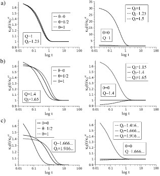
Figure 1: On the left column, the temporal evolution of $Q$-kurtosis for Itô ($\theta=0$), Stratonovich ($\theta=1/2$) and backward Itô ($\theta=1$) stochastic procedures. The numerical results are normalized by its stationary value $\kappa_{Q}^{st}=\kappa_{Q}(\infty)$. In (a) we have $Q=1$ and $Q_{i}=5/4$, in (b) $Q=7/5$ and $Q_{i}=1.65$ and (c) $Q=1.666...$ and $Q_{i}=1.91666...$ . As expected, for sufficient large times the numerical results approaches to unity. The right column shows the temporal evolution of the normalized $Q$-kurtosis with a fixed $\theta$. In (a) we have $Q=1$ and $Q_{i}=1,\,5/4\,\text{and}\,3/2$; (b) shows the results for $Q=7/5$ and $Q_{i}=1.15,\,7/5\,\text{and}\,1.65$; and (c) the results for $Q=5/3$ and $Q_{i}=1.41666...,\,5/3\,\text{and}\,1.91666...$ .

In Fig. 2 we can compare the behavior of the standard kurtosis and the $Q$-kurtosis given by Eq. (44). As we can see, the $Q$-kurtosis diverges at $Q=-1$, but is finite for $-1<Q<3$, while the standard kurtosis diverges for $7/5<Q<3$. As expected, the $Q$-kurtosis coincides with the standard one for $Q=1$. Furthermore, the $Q$-kurtosis is a monotonically decreasing function of $Q$. Based on this feature, experimentalists could use it as a calibration curve that allows the determination of the proper value of the entropic index $Q$ for a given system.

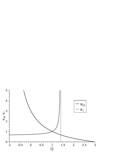
Figure 2: The standard kurtosis $\kappa_{1}$ and the $Q$-kurtosis $\kappa_{Q}$ as functions of $Q$. We verify that both have the same value 1 for $Q=1$. For $Q>1$, the use of $\kappa_{Q}$ is generically more convenient than using $\kappa_{1}$. Indeed, the latter one diverges at $Q=7/5$ while $\kappa_{Q}$ remains finite up to the maximal value $Q=3$. In contrast, for $Q<1$, $\kappa_{1}$ is more convenient than $\kappa_{Q}$. Indeed, $\kappa_{Q}$ diverges at $Q=-1$, whereas $\kappa_{1}$ remains finite down to $Q\to-\infty$. In the $Q\to-\infty$ limit, $\kappa_{1}$ saturates at the value $3/5$.

IV Conclusions

Based on stochastic integrals which unify Itô and Stratonovich approaches, we obtain (in two different though equivalent forms) an unified Fokker-Planck equation which recovers, as particular instances, equations currently available in the literature. Both Fokker-Planck forms exhibit an explicit dependence on the unifying parameter ($\theta$). One of these forms shows this dependence only in the deterministic part as a noise-induced drift term; in the other one, it only appears in the diffusion term. We present, based on escort mean values, an explicit form for the $Q$-generalized kurtosis to study the convergence towards the $Q$-Gaussian stationary solution. The difference in the convergence for the same $q$-Gaussian with different $\theta$’s is due to the change in the amplitude of the multiplicative noise needed to compensate the change in $\theta$ (see Eq. (24)). This is the origin of the difference in the convergence velocity when we keep $Q_{i}$’s and $Q$’s constant, and vary $\theta$. Looking at the time evolution of the $Q$-kurtosis starting from different initial conditions, i.e. different $Q_{i}$’s, we see that the convergence is reached for a little less than two decades in all explored cases. Finally, we propose that, if a system is well described by the nonextensive statistical mechanics, and has a $Q$-Gaussian form for its probability density function, the $Q$-kurtosis can be used as a calibration curve to determine, from data, the best value of the entropic index $Q$.

Appendix

IV.1 The integral $I_{\theta}[W(t)]=\int_{t_{0}}^{t}dW(t^{\prime})W(t^{\prime})$

Here we perform, in details, the calculation of the stochastic integral of the function $G(t)=W(t)$ in terms of discrete sums.

The definition of the unified stochastic integral is

$$I_{\theta}[G(t)]\equiv\text{ms -}\lim_{n\rightarrow\infty}S_{n}=\text{ms -}\lim_{n\rightarrow\infty}\sum_{i=1}^{n}\left[\theta G_{i}+(1-\theta)G_{i-1}\right]\Delta W_{i}\;.$$ (45)

If $G(t)=W(t)$, we have

$$S_{n}=\sum_{i=1}^{n}\left[\theta W_{i}\Delta W_{i}+(1-\theta)W_{i-1}\Delta W_{i}\right]\;.$$ (46)

The terms $W_{i}\Delta W_{i}$ and $W_{i-1}\Delta W_{i}$ can be written as

$$2W_{i}\Delta W_{i}=(W_{i})^{2}+(\Delta W_{i})^{2}-(\overbrace{W_{i}-\Delta W_{i}}^{W_{i-1}})^{2}$$ (47)

$$2W_{i-1}\Delta W_{i}=(\underbrace{W_{i-1}+\Delta W_{i}}_{W_{i}})^{2}-(W_{i-1})^{2}-(\Delta W_{i})^{2} \;.$$ (48)

Notice that in both equations we have terms like $(W^{2}_{i}-W^{2}_{i-1})$ under a summation. Therefore only the first and the last terms need to be taken into account in the summation. Indeed, all the others mutually cancel, and we will finally have

$$\sum_{i=1}^{n}W_{i}\Delta W_{i}=\frac{W^{2}(t)-W^{2}(t_{0})+\sum_{i=1}^{n}(\Delta W_{i})^{2}}{2}$$ (49)

$$\sum_{i=1}^{n}W_{i-1}\Delta W_{i}=\frac{W^{2}(t)-W^{2}(t_{0})-\sum_{i=1}^{n}(\Delta W_{i})^{2}}{2} \;.$$ (50)

Taking this last two equations into account and the fact that $\text{ms -}\lim_{n\rightarrow\infty}\sum_{i=1}^{n}(\Delta W_{i})^{2}=t-t_{0}$, we obtain

$$I_{\theta}[W(t)]\equiv\text{ms -}\lim_{n\rightarrow\infty}S_{n}=\frac{1}{2}\left\{[W(t)]^{2}-[W(t_{0})]^{2}-(1-2\theta)(t-t_{0})\right\}\;.$$ (51)

which is the same result presented in Eq. (5).

IV.2 How to get Eq. (15) from Eq. (16)

In section II we claim that Eqs. (15) and (16) are equivalent. To prove this statement, we only need to show the following equality:

$$K_{0}P-\frac{1}{2}[D]^{2\theta}\frac{\partial}{\partial u}\left\{[D]^{1-2\theta}P\right\}=K_{\theta}P-\frac{1}{2}\frac{\partial}{\partial u}\left[DP\right]\;,$$

where the dependence on the dynamical variable $u$ was omitted. To do this, we perform the derivative on the left hand side.

$$D^{2\theta}\frac{\partial}{\partial u}\left[D^{1-2\theta}P\right] = D^{2\theta}\left[(1-2\theta)D^{-2\theta}P\frac{\partial D}{\partial u}+D^{1-2\theta}\frac{\partial P}{\partial u}\right]$$ (52)

$$= -2\theta\frac{\partial D}{\partial u}P+\left[P\frac{\partial D}{\partial u}+D\frac{\partial P}{\partial u}\right]$$

$$= -2\theta\frac{\partial D}{\partial u}P+\frac{\partial}{\partial u}\left[DP\right]\;.$$

So,

$$K_{0}P-\frac{1}{2}[D]^{2\theta}\frac{\partial}{\partial u}\left\{[D]^{1-2\theta}P\right\} = K_{0}P-\frac{1}{2}\left\{-2\theta\frac{\partial D}{\partial u}P+\frac{\partial}{\partial u}\left[DP\right]\right\}$$ (53)

$$= K_{0}P+\theta\frac{\partial D}{\partial u}P-\frac{1}{2}\frac{\partial}{\partial u}\left[DP\right]\;,$$

where $K_{0}P+\theta\partial_{u}DP=K_{\theta}$.

IV.3 The equivalence between $\dot{u}=f(u)+g(u)\xi(t)+\eta(t)$ and $\dot{u}=f(u)+\tilde{g}(u)\zeta(t)$

Suppose two different Langevin equations for the stochastic processes $u(t)$, both with the same deterministic drift force $f(u)$ but different noise sources,

$$\dot{u} = f(u)+g(u)\xi(t)+\eta(t)$$ (54)

$$\dot{u} = f(u)+\tilde{g}(u)\zeta(t)\;.$$ (55)

The mean-value solution of both equations is

$$\langle u(t)\rangle=\int_{0}^{t}dt^{\prime}f(u)\;.$$ (56)

Let us calculate the variance corresponding to both equations. From the first one we obtain

$$\langle[u(t)-\langle u(t)\rangle]^{2}\rangle = \left\langle\int_{0}^{t}dt^{\prime}\int_{0}^{t}dt^{\prime\prime}\left\{g[u(t^{\prime})]\xi(t^{\prime})+\eta(t^{\prime})\right\}\left\{g[u(t^{\prime\prime})]\xi(t^{\prime\prime})+\eta(t^{\prime\prime})\right\}\right\rangle$$ (57)

$$= \int_{0}^{t}dt^{\prime}\int_{0}^{t}dt^{\prime\prime}\left\{g[u(t^{\prime})]g[u(t^{\prime\prime})]\underbrace{\langle\xi(t^{\prime})\xi(t^{\prime\prime})\rangle}_{=2M\delta(t^{\prime}-t^{\prime\prime})}+\underbrace{\langle\eta(t^{\prime})\eta(t^{\prime\prime})\rangle}_{=2A\delta(t^{\prime}-t^{\prime\prime})}\right.$$ (59)

$$\qquad\qquad\qquad\left.+g[u(t^{\prime})]\underbrace{\langle\xi(t^{\prime})\eta(t^{\prime\prime})\rangle}_{=0}+g[u(t^{\prime\prime})]\underbrace{\langle\xi(t^{\prime\prime})\eta(t^{\prime})\rangle}_{=0}\right\}$$

$$= \int_{0}^{t}dt^{\prime}\left\{2M\left\{g[u(t^{\prime})]\right\}^{2}+2A\right\}\;.$$ (60)

From the second one we obtain

$$\langle[u(t)-\langle u(t)\rangle]^{2}\rangle = \int_{0}^{t}dt^{\prime}\int_{0}^{t}dt^{\prime\prime}\tilde{g}[u(t^{\prime})]\tilde{g}[u(t^{\prime\prime})]\underbrace{\langle\zeta(t^{\prime})\zeta(t^{\prime\prime})\rangle}_{2C\delta(t^{\prime}-t^{\prime\prime})}$$ (61)

$$= \int_{0}^{t}dt^{\prime}2C\left\{\tilde{g}[u(t^{\prime})]\right\}^{2}\;.$$ (62)

If we want that both Langevin equations give us the same mean-squared value for the stochastic process $u(t)$, we must match the integrands of Eqs. (57) and (61). This leads to the following relation among noise terms:

$$\tilde{g}(u)=\sqrt{\frac{M[g(u)]^{2}+A}{C}}\;.$$ (63)

This result shows that Eqs. like (17) can be rewritten as in (19), with an effective multiplicative noise term given by Eq. (63).

References

- (1) C. W. Gardiner, Handbook of Stochastic Methods (Springer, Berlin, 1997).
- (2) H. Risken, The Fokker-Planck Equation. Methods of solutions and applications (Springer-Verlag, New York, 1984).
- (3) G. Germano, M. Politi, E. Scalas and R. L. Schilling, Phys. Rev. E 79, 066102 (2009).
- (4) A. W. C. Lau and T. C. Lubensky, Phys. Rev. E 76, 011123 (2007)
- (5) P. Lançon, G. Batrouni, L. Lobry and N. Ostrowsky, Physica A 304, 65 (2002)
- (6) P. Lançon, G. Batrouni, L. Lobry and, N. Ostrowsky, Euro-Phys. Lett. 54, 28 (2001).
- (7) L. Chung and Jean-Claude Zambrini, Monograph of the Portuguese Mathematical Society, Vol. 1, World Scientific Publishing Company, 2003; A. I. Ilin, R. Z. Khasminski, Theo. Prob. Appl. 9, 466 (1964); E. Nelson, Dynamical Theories of the Brownian Motion, (Princeton, University Press, Princeton, 1967); E. Nelson, Quantum Fluctuations, (Princeton University, Princeton, 1985.)
- (8) N. Dokuchaev, arXiv:0708.2497v1.
- (9) C. Anteneodo and C. Tsallis, J. Math. Phys. 44, 5194, (2003).
- (10) N. van Kampen, Stochastic Processes in Physics and Chemistry (North-Holland, Amsterdam, 1981).
- (11) N. van Kampen, J. of Stat. Phys. 24, 175, (1981).
- (12) V. Schwammle, E.M.F. Curado and F.D. Nobre, Eur. Phys. J. B 58, 159 (2007); V. Schwammle, F.D. Nobre and E.M.F. Curado, Phys. Rev. E 76, 041123 (2007).
- (13) L. Borland, F. Pennini, A. R. Plastino and A. Plastino, Eur. Phys. J. B 12, 285 (1999).
- (14) C. Beck and F. Schlogl, Thermodynamics of Chaotic Systems (Cambridge University Press, Cambridge, 1993).
- (15) C. Tsallis, R. S. Mendes and A. R. Plastino, Physica A 261 534 (1998).
- (16) C. Tsallis, J. Stat. Phys. 52, 479 (1988); C. Tsallis, Introduction to Nonextensive Statistical Mechanics - Approaching a Complex World (Springer, New York, 2009).
- (17) A. Upadhyaya, J.-P. Rieu, J.A. Glazier and Y. Sawada, Physica A 293, 549 (2001).
- (18) A.M. Reynolds, Physica A 389, 273-277 (2010).
- (19) K.E. Daniels, C. Beck and E. Bodenschatz, Physica D 193, 208 (2004).
- (20) R. Arevalo, A. Garcimartin and D. Maza, Eur. Phys. J. E 23, 191-198 (2007)[DOI10.1140/epje/i2006-10174-1].
- (21) R. Arevalo, A. Garcimartin and D. Maza, A non-standard statistical approach to the silo discharge, in Complex Systems - New Trends and Expectations, eds. H.S. Wio, M.A. Rodriguez and L. Pesquera, Eur. Phys. J.-Special Topics 143 (2007) [DOI: 10.1140/epjst/e2007-00087-9].
- (22) P. Douglas, S. Bergamini and F. Renzoni, Phys. Rev. Lett. 96, 110601 (2006); G.B. Bagci and U. Tirnakli, Chaos 19, 033113 (2009).
- (23) B. Liu and J. Goree, Phys. Rev. Lett. 100, 055003 (2008).
- (24) R.G. DeVoe, Phys. Rev. Lett. 102, 063001 (2009).
- (25) L. Borland, Phys. Rev. Lett. 89, 098701 (2002).
- (26) L. Borland, Quantitative Finance 2, 415 (2002).
- (27) S.M.D. Queiros, Quant. Finance 5, 475-487 (2005).
- (28) L.F. Burlaga and A.F.-Vinas, Physica A 356, 375 (2005).
- (29) L.F. Burlaga and N.F. Ness, Astrophys. J. 703, 311-324 (2009).
- (30) B. Bakar and U. Tirnakli, Phys. Rev. E 79, 040103(R) (2009).
- (31) F. Caruso, A. Pluchino, V. Latora, S. Vinciguerra and A. Rapisarda, Phys. Rev. E 75, 055101(R)(2007).
- (32) L.G. Moyano and C. Anteneodo, Phys. Rev. E 74, 021118 (2006).
- (33) J.C. Carvalho, R. Silva, J.D. do Nascimento and J.R. de Medeiros, Europhys. Lett. 84, 59001 (2008).
- (34) CMS Collaboration, J. High Energy Phys. 02, 041 (2010).
- (35) R.M. Pickup, R. Cywinski, C. Pappas, B. Farago and P. Fouquet, Phys. Rev. Lett. 102, 097202 (2009).
- (36) V. Schwammle, F. D. Nobre and C. Tsallis, Eur. Phys. J. B 66, 537 (2008).
- (37) C. Tsallis, A. R. Plastino and R. F. Alvarez-Estrada, J. Math. Phys. 50, 043303 (2009).
- (38) S. Umarov, C. Tsallis an S. Steiberg, Milan J. of Mathematics 76, 307 (2008); S. Umarov, C. Tsallis, M. Gell-Mann and S. Steinberg, J. Math. Phys. 51, 033502 (2010).