Renormalization group theory for finite-size scaling in extreme statistics

Abstract

We present a renormalization group (RG) approach to explain universal features of extreme statistics, applied here to independent, identically distributed variables. The outlines of the theory have been described in a previous Letter, the main result being that finite-size shape corrections to the limit distribution can be obtained from a linearization of the RG transformation near a fixed point, leading to the computation of stable perturbations as eigenfunctions. Here we show details of the RG theory which exhibit remarkable similarities to the RG known in statistical physics. Besides the fixed points explaining universality, and the least stable eigendirections accounting for convergence rates and shape corrections, the similarities include marginally stable perturbations which turn out to be generic for the Fisher-Tippett-Gumbel class. Distribution functions containing unstable perturbations are also considered. We find that, after a transitory divergence, they return to the universal fixed line at the same or at a different point depending on the type of perturbation.

I Introduction

Using present data-acquisition methods, it has become possible to build enormous databases in practically all fields of science. The large size of these databases make their analysis rather intricate, but questions can now be posed which were previously unanswerable. In particular, quantitative studies of extreme events have become feasible. Accordingly, extreme value statistics (EVS) has found its way from mathematics Fisher and Tippett (1928); Gumbel (1958) to various disciplines, foremost among them those fields where the extremes involve great risks as in engineeringWeibull (1951), finance Embrecht et al. (1997), hydrology Katz et al. (2002), meteorology v. Storch and Zwiers (2002), geology Gutenberg and Richter (1944). In physics, extreme statistics was relatively dormant until the last decade when a number of studies appeared in relation to spin glasses Bouchaud and Mézard (1997), interface– and landscape–fluctuations Raychaudhuri et al. (2001); Antal et al. (2001); Györgyi et al. (2003); Le Doussal and Monthus (2003); Majumdar and Comtet (2004, 2005); Bolech and Rosso (2004); Guclu and Korniss (2004), random fragmentation Krapivsky and Majumdar (2000), level-density in ideal quantum gases Comtet et al. (2007), atmospheric time series Eichner et al. (2006), etc.

The above studies revealed that an important problem with the quantitative application of EVS is the slow convergence in the size $N$ of the data set whose extremum is sought. A well known example is that the Fisher-Tippett-Gumbel limit distribution for independent, identically distributed (i.i.d.) variables is typically approached logarithmically slowly, i.e. proportionally to $1/\ln N$. This convergence problem is not cured even by the present size of the databases, thus studies of finite-size corrections are needed for a thorough analysis of EVS. While the mathematical literature contains results on the rate of convergence to the universal limit distributions de Haan and Resnick (1996); de Haan and Stadtmüller (1996), and particular cases for correlated variables have also been studied in physics Schehr and Majumdar (2006), to our knowledge, finite-size effects have apparently been ignored in most empirical data analysis.

In order to develop a readily usable theory of finite-size corrections giving not only the amplitude of the corrections but also providing shape corrections to the limit distribution, we recently introduced a renormalization group (RG) approach for the case of i.i.d. variables Györgyi et al. (2008). The concept of using RG in probability theory has been pioneered by Jona-Lasinio Jona-Lasinio (2001) in connection with critical phenomena. In the context of EVS, the real-space RG methods have been applied to random landscapes Le Doussal and Monthus (2003); Schehr and Le Doussal (2009). In our case, it turned out that the RG equation is just a physicist’s reformulation and a simple generalization of the original fixed point equation of Fisher and Tippett Fisher and Tippett (1928). Within this approach, the fixed point condition yields the known one-parameter ($\gamma$) family of solutions which provides the traditional classification of EVS limit distributions (Fisher-Tippett-Gumbel, -Fréchet, -Weibull). The RG approach is instrumental in determining the finite-size corrections as well, since they emerge from the action of the RG on the neighborhood of the fixed point. We found that the resulting eigenvalue problem and the emerging eigenfunctions represent the generic leading finite-size correction functions. An important outcome of the general considerations is that the first order shape corrections display universality. Namely, within a class of limit distributions characterized by $\gamma$, the correction is determined by a single additional parameter $\gamma^{\prime}$. The $\gamma$ is long known to be related to the leading asymptote of the parent distribution, while $\gamma^{\prime}$, emerging as an eigenvalue index from RG, is determined by the next-to-leading asymptote of the parent distribution which is in accordance with the mathematical results de Haan and Resnick (1996); de Haan and Stadtmüller (1996). Note that our RG framework also provides a simple example in addition to a series of known exact RG schemes Jona-Lasinio (2001); Ma (1973); Hilhorst et al. (1978); McKay et al. (1982); Schuster and Just (2005).

The above RG picture and the corresponding results have been briefly presented in a recent Letter Györgyi et al. (2008). Here, we offer an extended and more detailed view on our work with new aspects relating to the nonlinear neighborhood of the fixed line including nonlinear manifolds. In particular, a detailed derivation of the RG picture is presented in Sec. II where the fixed line of the RG transformation, parametrized by $\gamma$, is linked to the EVS limit distributions. Next, linear perturbations around a point on the fixed line are considered. The eigenvalue problem is solved (Sec. III), giving rise to a new parameter $\gamma^{\prime}$. The general aspects of the theory are developed further in Sec. IV where the RG transformation beyond the linear neighborhood of the fixed point is formulated to treat the case of marginal eigenfunctions within the Fisher-Tippett-Gumbel class. The practical consequences are discussed by connecting to the finite size properties in typical EVS problems and showing that the parameter $\gamma^{\prime}$ is the finite-size scaling exponent (Sec. V). Furthermore, the relationship between $\gamma^{\prime}$ and the parent distributions is determined, and we analyze in detail a family of parents with generalized exponential asymptote frequently occuring in applications. The question of unstable perturbations and the invariant manifolds associated with them are examined in Sec. VI, and they are illustrated on a series of examples. Finally, the conclusion and possible avenues for further application of the RG scheme to EVS problems are found in Sec. VII.

II Renormalization group transformation and its fixed line

In this section we recuperate known basic properties of EVS and explain the emergence of limit distributions within the framework of RG theory. This is essentially a reformulation of the original proposition of the seminal work by Fisher and Tippett Fisher and Tippett (1928), which we will further develop in subsequent sections.

The basic question of EVS is the limit behavior of the distribution of extremal values of random variables. In what follows we shall restrict our attention to maxima, i.e., the distribution of the largest variable, but by a sign change this is equivalent to the problem of minima. Suppose that we have a “batch” of random variables $z_{1},z_{2},\dots,z_{N}$, and we ask about the statistical properties of the largest $z=\max{\left\{z_{1},z_{2},\dots,z_{N}\right\}}$. The question has a simple answer, if the original variables $z_{i}$ were independent, identically distributed, each according to the so called parent probability density $\rho(z)$. The simplicity is apparent when using the integrated (cumulative) distribution

$$\mu(z)=\int_{-\infty}^{z}\!\rho(\bar{z})d\bar{z},$$ (II.1)

i.e. the probability that the variable is not larger than $z$ (we assume here and later nonsingular densities, and differentiability if necessary). Then the probability that the maximum is not exceeding $z$ is given by the joint probability that all variables do not exceed $z$, hence the integrated distribution of the maximum of batch of $N$ variables, the extreme value distribution (EVD) is

$$M_{N}^{\max}(z)=\mu^{N}(z).$$ (II.2)

Since the integrated parent distribution $\mu(z)$ is less than one whenever $z$ is within the support of the parent, the above quantity will converge to zero there for any fixed $z$. However, we can ask whether there is a linear change of variable so that for large $N$ the EVD is restored to a nondegenerate function in the large $N$ limit. Specifically, we ask about the existence of parameters $a_{N},b_{N}$ such that

$$M_{N}(x)=M_{N}^{\max}(a_{N}x+b_{N})\to M(x),$$ (II.3)

where the resulting integrated distribution represents the extreme value limit distribution. It is related to the limit density as $P(x)=M^{\prime}(x)$.

Note that the parameters $a_{N},b_{N}$ are not unique, if one choice produces a nondegenerate limit EVD then adding constants to either will also yield another one. This ambiguity can be eliminated by a standardization convention, for example

$$M(0)=P(0)=1/e.$$ (II.4)

We can require this condition also at finite stages in the limit (II.3) for the maximum distribution $M_{N}(x)$, which specifies uniquely the parameters $a_{N},b_{N}$.

Now let us turn to the invariance condition, which follows from the fact that $M(x)$ is a limit distribution of EVS. The reason behind this invariance is that if $p$ variables come from a parent that is a limit EVD, then their maximum will be also distributed according to the same limit EVD. Indeed, conceiving each of the variables as themselves representing maxima of some other large collection of variables, the distribution of their overall maximum will obviously be again the same limit EVD. Since these statements are valid up to a linear change of variable, for the limit EVD we obtain

$$M(x)=M^{p}(a(p)x+b(p)),$$ (II.5)

with appropriate scale- and shift paramenters, $a(p)$ and $b(p)$. While here $p$ should be a positive integer, we can easily convince ourselves that it can be any positive rational. Indeed, considering another $N^{\prime}=Np$, where $p$ is fixed during the large size limit, and making use of

$$M_{N}(x)\approx M_{Np}(x),$$ (II.6)

we obtain by (II.2,II.3) again (II.5). Then $p$ can in fact be continued to positive real numbers. The parameters $a(p),b(p)$ in (II.5) should be consistent with the standardization (II.4). In sum, condition (II.5) should be understood such that if $M(x)$ is a limit distribution then it should solve (II.5) for any $p$ with parameters ensuring (II.4). This is known in the mathematical literature as the condition of max-stability, appearing first in the classic paper by Fisher and Tippett Fisher and Tippett (1928) and now an exercise in textbooks on EVS.

In order to go later beyond the invariance condition, following our short paper Györgyi et al. (2008), we will identify the RG transformation of an integrated distribution $\mu(x)$ by the following operation

$$[\hat{R}_{p}\mu](x) =\mu^{p}(a(p)x+b(p)).$$ (II.7)

One can easily see that the standardization of the type (II.4) for $[\hat{R}_{p}\mu](x)$ requires

$$b(p) =\mu^{-1}(e^{-1/p}),$$ (II.8a)

$$a(p) =p\frac{d\,b(p)}{dp},$$ (II.8b)

​​​a condition forming part of the RG operation. Note that traditional RG used in critical phenomena is in fact a semigroup since, due to the elimination of degrees of freedom, the inverse element is missing. In our case, however, the transformations form a group, as the inverse element of a transformation with parameter $p$ has parameter $1/p$. Obviously, $p<1$ corresponds to the decrease of the batch size, but the above RG transformation is still meaningful.

We should note that, although there are differences, the EVS version of the RG transformation [eqs.(II.7,II.8)] has the spirit of the traditional RG. Namely, the raising to power $p>1$ and shifting by $b(p)$ decreases the weight of the small argument part of the parent distribution (eliminating the irrelevant degrees of freedom), while rescaling by $a(p)$ is analogous to the rescaling of the remaining degrees of freedom.

Within RG theory, the invariance condition (II.5) becomes a fixed point relation

$$[\hat{R}_{p}M](x)=M(x).$$ (II.9)

Concerning terminology, we mention that while in mathematical texts max-stability is essentially the fixed point relation, in the RG framework stability is characterized by the response to small deviations from the fixed point, to be investigated later in the paper.

One can easily solve (II.9) by introducing the function $f(x)$ as

$$M(x)=e^{-e^{-f(x)}},$$ (II.10)

where standardization (II.4) requires

$$f(0)=0,\,\ \ f^{\prime}(0)=1,$$ (II.11)

furthermore, from (II.8) the parameters can be written in terms of $f$ as

$$b(p) =f^{-1}(\ln p),$$ (II.12a)

$$a(p) =1/f^{\prime}(b(p)).$$ (II.12b)

The equation for $f$ can be obtained from (II.9), that is, writing (II.5) as

$$f(x) =f(a(p)x+b(p))-\ln p$$ (II.13)

whence

$$f^{\prime}(x) =a(p)f^{\prime}(a(p)x+b(p)).$$ (II.14)

It follows that the sought solution for $f^{\prime}$, independent of $p$, is the reciprocal of a linear function. The only form consistent with (II.11) allows one free parameter, $\gamma$, yielding

$$f^{\prime}(x;\gamma) =\frac{1}{1+\gamma x},$$ (II.15)

where here and later ^′ means differentiation by $x$, and $b(p)=\gamma^{-1}(a(p)-1)$ should hold. Again using (II.11) we get by integration the one-parameter family

$$f(x;\gamma)=\gamma^{-1}\ln(1+\gamma x),$$ (II.16)

and (II.12) requires

$$a(p,\gamma) =p^{\gamma},$$ (II.17a)

$$b(p,\gamma) =\gamma^{-1}(p^{\gamma}-1).$$ (II.17b)

Equation (II.16) gives with (II.10) the well known generalized extreme value distribution and the respective density

$$M(x;\gamma) =e^{-(1+\gamma x)^{-1/\gamma}}$$ (II.18a)

$$P(x;\gamma) =(1+\gamma x)^{-1/\gamma-1}e^{-(1+\gamma x)^{-1/\gamma}},$$ (II.18b)

​​with support extending to the range $1+\gamma x\geq 0$. This one-parameter family constitutes a fixed line of the RG transformation. The cases $\gamma<0,\,=0,\ >0$ were studied separately already by Fisher and Tippett Fisher and Tippett (1928), and correspond to the traditional categorization into Weibull, Gumbel, and Fréchet universality classes, respectively. The $\gamma<0$ case gives the limit distribution of integrated parent distributions approaching $1$ like a power $-1/\gamma$ at a finite upper border, $\gamma=0$ corresponds to faster than power asymptote at either a finite limit or at infinity, and $\gamma>0$ represents parent distributions approaching $1$ at infinity with a power $-1/\gamma$. These three cases will be referred to by the abbreviations FTW, FTG, and FTF, respectively.

III Eigenvalue problem near the fixed point

III.1 Perturbation about the fixed point

While the above fixed point condition is a textbook example of deriving the limit distributions of EVS, its perturbation has not been studied. Nevertheless, such perturbations are important since they naturally give rise to finite-size corrections. Before elucidating the connection to finite-size scaling, let us consider the function space about the fixed point and its transformations under the RG operation represented by the right-hand-side of (II.5). Introduce the perturbed distribution function

$$M(x;\gamma,\epsilon)=M(x+\epsilon\psi(x);\gamma),$$ (III.1)

where $M(x;\gamma)$ is assumed to satisfy the fixed point condition. We insert the perturbation into the argument since this leads to a simpler formulation later. Alternatively, one can also define

$$M(x;\gamma,\epsilon)=M(x;\gamma)+\epsilon P(x;\gamma)\psi(x).$$ (III.2)

The two formulas are equivalent to linear order in $\epsilon$. On the other hand, for a given finite $\epsilon$ the monotonicity condition for the integrated distribution $M(x;\gamma,\epsilon)$ in $x$ may impose different restrictions on $\psi(x)$. Generically, both formulas can be understood as approximations for small $\epsilon$ of some distribution with general $\epsilon$ dependence, sufficient for the present purposes. If we consider finite perturbations, that will be explicitly stated and the monotonicity condition discussed.

The standardization condition of the type (II.4) for both of the above integrated distribution functions is satisfied by

$$\psi(0)=0,\,\psi^{\prime}(0)=0,\ \psi^{\prime\prime}(0)=-1.$$ (III.3)

The third condition sets the sign and scale of $\epsilon$, the minus sign is just a convention which will be justified later. Note that in our short communication Györgyi et al. (2008) we used $\psi^{\prime\prime}(0)=1$, so in comparisons a sign change should be understood.

III.2 Eigenvalues and eigenfunctions

Now we shall study the eigenvalue problem of the linearized RG transformation around the fixed point, specifically, when the RG transformation changes the magnitude of the perturbation while leaving its functional form invariant. In other words, we are seeking the linear part of the invariant manifold of the RG emanating from the fixed point.

To make notation simpler in this section, we often omit the $\gamma$ and $p$ arguments, when they are obviously implied, e.g., we use $M(x;\epsilon)$ for $M(x;\gamma,\epsilon)$, etc. We start out from (III.1), apply the RG transformation, and assume that the result is of the same functional form with only the perturbation parameter changing

$$[\hat{R}_{p}M(\epsilon)](x)=M^{p}(a(\epsilon)x+b(\epsilon);\epsilon)=M(x;\epsilon^{\prime}),$$ (III.4)

where linearization in $\epsilon$ and $\epsilon^{\prime}$ is understood. The transformation parameters are also expanded

$$a(\epsilon) =a+\epsilon a_{1},$$ (III.5a)

$$b(\epsilon) =b+\epsilon b_{1},$$ (III.5b)

with the zeroth order values $a,b$ taken from (II.17) and the first order corrections $a_{1},\,b_{1}$ to be determined from the standardization condition (II.8) with $\mu(x)=M(x;\epsilon)$. Using (III.1) and (II.10) in these conditions we straightforwardly get

$$b_{1} =-\psi(b)$$ (III.6a)

$$a_{1} =-\psi^{\prime}(b)a.$$ (III.6b)

​​What is left is to determine the possible values of $\epsilon^{\prime}$ and the associated invariant function $\psi(x)$.

We now use (II.16) and (II.10), expand to linear order in $\epsilon$ and $\epsilon^{\prime}$ in the second exponential, and introduce their ratio as eigenvalue

$$\lambda=\epsilon^{\prime}/\epsilon.$$ (III.7)

Then we obtain

$$\begin{split}\lambda a\psi(x)&=\psi(ax+b)+a_{1}x+b_{1}\\ &=\psi(ax+b)-\psi(b)-a\psi^{\prime}(b)x.\end{split}$$ (III.8)

We used (III.6) to obtain the second line, which makes it obvious that the rôle of the constants $a_{1},b_{1}$ is to ensure the first two conditions in (III.3).

By differentiation we can eliminate the linear part

$$(\lambda/a)\psi^{\prime\prime}(x)=\psi^{\prime\prime}(ax+b)$$ (III.9)

We remind the reader that $a,b$ are given in (II.17) and change continuously with $p$, furthermore, we recall that

$$1+\gamma(ax+b)=a(1+\gamma x).$$ (III.10)

Thus the $p$ independent solution is

$$\psi^{\prime\prime}(x) =-(1+\gamma x)^{\alpha},$$ (III.11)

where the coefficient $-1$ follows from the third condition in (III.3), and the eigenvalue is obtained as

$$\lambda =a^{\alpha+1}=p^{\gamma(\alpha+1)},$$ (III.12)

where we also used (II.17a). The parameter $\alpha$ labels the eigenfunctions, but it is more convenient to introduce $\gamma^{\prime}=\gamma(\alpha+1)$, which gives

$$\psi^{\prime\prime}(x;\gamma,\gamma^{\prime}) =-(1+\gamma x)^{\gamma^{\prime}/\gamma-1},$$ (III.13)

$$\lambda(\gamma^{\prime}) =p^{\gamma^{\prime}}.$$ (III.14)

Linear stability of the fixed point for $p>1$ means that $\lambda<1$, then $\gamma^{\prime}<0$, the marginal case is $\lambda=1,\gamma^{\prime}=0$, while $\lambda>1,\gamma^{\prime}>0$ characterizes unstable directions.

The eigenfunction is obtained by integrating eq.(III.11) while satisfying the conditions (III.3)

$$\begin{split}\psi(x;\gamma,\gamma^{\prime})&=-\int_{0}^{x}dy\int_{0}^{y}dz\,(1+\gamma z)^{\gamma^{\prime}/\gamma-1}\\ &=\frac{1+(\gamma^{\prime}+\gamma)x-(1+\gamma x)^{\gamma^{\prime}/\gamma+1}}{\gamma^{\prime}(\gamma^{\prime}+\gamma)}.\end{split}$$ (III.15)

Note that for $\gamma=\gamma^{\prime}$ (III.15) simplifies to

$$\psi(x;\gamma,\gamma)=-\frac{x^{2}}{2}$$ (III.16)

irrespective of the value of $\gamma$. A function equivalent to (III.15) has been found in de Haan and Resnick (1996); Gomes and de Haan (1999) when studying convergence to the limit distribution, after starting out with parent distributions in the appropriate domain of attraction.

Knowing $\psi$, a substitution in (III.6) yields the corrections to the parameters as

$$a_{1} =\frac{p^{\gamma}(p^{\gamma^{\prime}}-1)}{\gamma^{\prime}},$$ (III.17a)

$$b_{1} =\frac{p^{\gamma+\gamma^{\prime}}}{\gamma^{\prime}(\gamma+\gamma^{\prime})}-\frac{p^{\gamma}}{\gamma\gamma^{\prime}}+\frac{1}{\gamma(\gamma+\gamma^{\prime})}.$$ (III.17b)

Summing up this section, we found using the RG theory that, for each fixed point specified by a $\gamma$, the linearized RG transformation yields a one-parameter family of eigenfunctions $\psi(x;\gamma,\gamma^{\prime})$. The rôle of the index $\gamma^{\prime}$ will be elucidated below in Sec.V.

III.3 Marginal eigenfunctions

We can immediately surmise that marginal eigenfunctions should appear on the line of fixed points $f(x;\gamma)$ (II.16). Since two fixed point functions stay the same upon the action of the RG transformation, their difference is also invariant with respect to the RG. If, in particular, the difference function was small, i.e., the two fixed points were differing by an infinitesimal increment in $\gamma$, then the difference function can be considered as a linear perturbation about either fixed point and, based on its invariance upon the RG, it should be proportional to the marginal eigenfunction with eigenvalue $\lambda=1$. By (III.14) this implies $\gamma^{\prime}=0$, whence we conclude that $\psi(x;\gamma,0)$ should emerge as an eigenfunction.

The above reasoning is confirmed by a simple calculation. First we display the marginal eigenfunction from (III.15)

$$\begin{split}\psi(x;\gamma,0)&=\gamma^{-2}\left[\gamma x-(1+\gamma x)\ln(1+\gamma x)\right].\end{split}$$ (III.18)

On the other hand, let us invoke the fixed point distribution (II.18a) and expand to leading order in $\gamma-\gamma_{0}$ about some nearby $\gamma_{0}$. It is easy to see that

$$\frac{\partial}{\partial\gamma}M(x;\gamma)=P(x;\gamma)\,\psi(x;\gamma,0),$$ (III.19)

with the definition (III.18), so finally we obtain for the perturbed fixed point

$$M(x;\gamma) \approx M(x;\gamma_{0})+\epsilon P(x;\gamma_{0})\,\psi(x,\gamma_{0},0),$$ (III.20a)

$$\epsilon =\gamma-\gamma_{0}.$$ (III.20b)

A comparison with (III.2) shows that indeed the difference of two infinitesimally close fixed point distributions is given by the marginal eigenfunction. This is interesting also from the viewpoint that one can determine the marginal function without solving the eigenvalue problem, by differentiation in terms of $\gamma$. Presumably for non-marginal functions it remains necessary to consider the traditional eigenvalue equation.

As a side-remark, the scale and sign of the eigenfunctions (III.15) were defined by the requirement (III.3). This had the consequence that the perturbation formula (III.20) has as small parameter $\epsilon$ just the increment in $\gamma$. Any other convention for the curvature at the origin in (III.3) would have introduced an extra factor in the perturbation in (III.20a), so the prescription (III.3) indeed provides the most natural scale and sign of the eigenfunctions.

IV Beyond linearized RG in the marginal case

Here we shall deal with the situation when $\gamma^{\prime}=0$, i.e., from (III.14) the eigenvalue $\lambda=1$, so within linear theory the size of the perturbation does not change under the action of the RG transformation. That is, the perturbation with such an eigenfunction is marginal, and we have to extend the RG formulation to terms nonlinear in $\epsilon$.

For the fixed point with nonzero $\gamma$, when the parent distribution has a power asymptote, the case of $\gamma^{\prime}=0$ seems to be atypical, because $\psi(x;\gamma,0)$ has a logarithmic singularity as shown in (III.18). On the other hand, in the FTG class with $\gamma=0$ the case $\gamma^{\prime}=0$ can be considered as generic, because the correction function $\psi(x;0,0)=-x^{2}/2$ represents the natural analytic perturbation in (III.1). We shall thus limit the RG study in the nonlinear neighborhood of the fixed line to the FTG case. Consider the most natural extension of (III.1) with $\gamma=\gamma^{\prime}=0$ (these arguments will be omitted in this section) as

$$M(x;\epsilon)=M(x-\epsilon x^{2}/2+\epsilon^{2}\psi_{2}(x)),$$ (IV.1)

where $M(x)=e^{-e^{-x}}$ and we require

$$\psi_{2}(0)=\psi_{2}^{\prime}(0)=\psi_{2}^{\prime\prime}(0)=0\,,$$ (IV.2)

where the first two equations follow from the standardization condition (II.4) while the third one sets the scale of $\epsilon$.

The RG transformation is again given by (III.4) where the right-hand-side should be expanded to second order in $\epsilon$ and

$$a(\epsilon) =1+\epsilon\ln p+\epsilon^{2}a_{2},$$ (IV.3a)

$$b(\epsilon) =\ln p+\frac{\epsilon}{2}\ln^{2}p+\epsilon^{2}b_{2}\,.$$ (IV.3b)

Here the terms up to linear order in $\epsilon$ were taken from the $\gamma,\gamma^{\prime}\to 0$ limit of (II.17). Since by (III.14) the eigenvalue is now $\lambda=1$, i.e., the eigenfunction is marginal to linear order, we assume an analytic extension of $\epsilon^{\prime}=\lambda\epsilon$ as

$$\epsilon^{\prime}=\epsilon-r\epsilon^{2}.$$ (IV.4)

Nonlinear stability then requires $|\epsilon^{\prime}|<|\epsilon|$, thus $r\epsilon>0$. If $r\epsilon<0$ then we have an unstable direction.

Straightforward calculation based on the RG transformation of (III.4) together with (IV.3,IV.4) yields

$$\psi_{2}^{\prime\prime}(x+\ln p)=\psi_{2}^{\prime\prime}(x)+2\ln p+r.$$ (IV.5)

The $p$-independent solution $\psi$ of this equation is linear

$$\psi_{2}^{\prime\prime}(x) =sx,$$ (IV.6)

where $s$ is arbitrary, and $r$ is determined as

$$r =(s-2)\ln p.$$ (IV.7)

Hence

$$\epsilon^{\prime}=\epsilon-\epsilon^{2}(s-2)\ln p,$$ (IV.8)

and using (IV.2) we obtain

$$\psi_{2}(x;s)=\frac{s}{6}x^{3}.$$ (IV.9)

Thus we find that in this order a new additional parameter $s$ arises. The corrections to the transformation parameters can also be calculated as

$$a_{2} =\frac{3-s}{2}\ln^{2}p,$$ (IV.10)

$$b_{2} =\frac{3-s}{6}\ln^{3}p.$$ (IV.11)

Nonanalytic corrections dominating the quadratic in $\epsilon$ can studied by the ansatz

$$\epsilon^{\prime}=\epsilon-r|\epsilon|^{\xi},\ \ \ 1<\xi<2.$$ (IV.12)

Carrying out an analysis similar to the above one, we again obtain the cubic eigenfunction (IV.9) but now $r=s\ln p$.

Next, the above results will be used to obtain practicable finite-size expressions in EVS.

V Finite size scaling

So far we have been studying the abstract space of distribution functions under the action of the RG transformation. Below we explain how the results on the eigenfunctions near a fixed point can be translated to the size dependence of the convergence to the limiting EVD starting out from a particular parent distribution.

V.1 The finite-size exponent $\gamma^{\prime}$

Consider the basic situation described in Sec. II, namely, the EVD $M_{N}(x)$ approaches one of the fixed points $M(x;\gamma)$ for a diverging batch size $N$. Then it is natural to assume that the convergence for large $N$ occurs along a dominant eigenfunction, approximated by the form (III.1), with some $\epsilon=\epsilon_{N}$. Further $p$ iterates of the extreme value distribution by the RG transformation corresponds to increasing the batch size to $pN$, and so, according to (III.4), it generates a new perturbation parameter

$$\epsilon^{\prime}=\epsilon_{pN}=\lambda_{\gamma^{\prime}}\epsilon_{N}.$$ (V.1)

Using now $\lambda(\gamma^{\prime})=p^{\gamma^{\prime}}$ (III.14) and assuming a power law dependence for $\epsilon_{N}$, one obtains

$$\epsilon_{N}\propto N^{\gamma^{\prime}}.$$ (V.2)

Hence the meaning of the parameter $\gamma^{\prime}$ follows, it is the exponent of the leading finite-size correction to the limit distribution. Clearly, $\gamma^{\prime}<0$ is needed for power-like decay whereas a correction faster or slower than power-law should be characterized within the RG theory of linear perturbations by a $\gamma^{\prime}=-\infty$ and $\gamma^{\prime}=0$, respectively.

V.2 Marginal case near the FTG fixed point

One expects that slower than power such as logarithmic corrections are also consistent with (V.1) and they emerge in the $\gamma^{\prime}\to 0$ limit. We study this case by considering the marginal situation near the FTG fixed point, as described in Sec. IV. Again we take an $\epsilon_{N}$ function, and get in one RG step $\epsilon^{\prime}=\epsilon_{pN}$. Expanding the reciprocal of (IV.8) yields in leading order

$$\frac{1}{\epsilon_{pN}}=\frac{1}{\epsilon_{N}}+(s-2)\ln p.$$ (V.3)

This is a functional equation for $1/\epsilon_{N}$, whose solution is the logarithm function, yielding

$$\epsilon_{N}\approx\frac{1}{(s-2)\ln N}.$$ (V.4)

Thus in the case $\gamma=\gamma^{\prime}=0$ the natural assumption of analyticity in $\epsilon$ leads to the cubic next-to-leading correction, and entails the logarithmic decay of the finite-size correction. This can be considered as the generic stable manifold about the FTG fixed point and explains the typically slow, $1/\ln N$, decay of the corrections.

Note that the above results consistently describe stable perturbations. Indeed, (IV.8) gives an $\epsilon^{\prime}$ closer to zero than $\epsilon$, if $\epsilon$ has the same sign as $s-2$. But this is just what we obtained in (V.4).

A more general case is when the nonlinear extension in the marginal situation is (IV.12). Translating that to the finite-size correction we have in the end

$$\epsilon_{N} \approx\frac{A}{(\ln N)^{\frac{1}{\xi-1}}},$$ (V.5)

$$A =\frac{\text{sgn}(s)}{[|s|(\xi-1)]^{\frac{1}{\xi-1}}}.$$ (V.6)

Hence RG theory accounts for faster-than-logarithmic decay in the case of an invariant manifold nonanalytic in $\epsilon$.

The conclusions drawn from the results of the RG study beyond the linear region are quite revealing. The correction characterizes how fast the parent distribution approaches the FTG fixed point. A quite slow but typical case is when the parent is attracted by the RG transformation to an invariant manifold analytic in both $x$ and the perturbation parameter $\epsilon$, yielding a finite-size correction logarithmically decaying in $N$. If the $\epsilon$-dependence is not analytic in next-to-leading order then a larger power of the log and so faster decay is obtained. These cases correspond to $\gamma^{\prime}=0$ and polynomial corrections in $x$, quadratic in leading and cubic in next-to-leading order. Faster, essentially power-law correction is obtained if the convergence is characterized by $\gamma^{\prime}<0$, when the correction function is no longer polynomial. Finally, faster than power decay corresponds to the case $\gamma^{\prime}\to-\infty$, thus it falls beyond the validity of the present RG theory.

V.3 Connection to the parent distribution

It remains to be seen how the perturbation parameter $\epsilon_{N}$ can be determined from the parent distribution. That is, we start out from the classic extreme value problem of the distribution of the maximum of $N$ i.i.d. variables, each characterized by the same parent distribution. Let us write the integrated parent distribution as

$$\mu(z)=e^{-e^{-g(z)}},$$ (V.7)

then the distribution of the maximum of $N$ variables is

$$M^{\max}_{N}(z)=\mu(z)^{N}=e^{-Ne^{-g(z)}}.$$ (V.8)

Let us assume that $\mu(z)$ belongs to the domain of attraction of the fixed point distribution $M(x;\gamma)$ from (II.18a). Then, by using the linear transformation ensuring the standardization (II.4)

$$z =a_{N}x+b_{N},$$ (V.9)

$$g(b_{N}) =\ln N,$$ (V.10)

$$g^{\prime}(b_{N}) =1/a_{N},$$ (V.11)

one obtains

$$M^{\max}_{N}(a_{N}x+b_{N})=M_{N}(x)\to M(x;\gamma).$$ (V.12)

Our basic assumption is that for large but finite $N$ the approach to the fixed point goes along some eigendirection as

$$M_{N}(x)\approx M(x+\epsilon_{N}\psi(x;\gamma,\gamma^{\prime});\gamma).$$ (V.13)

Here $\epsilon_{N}$ gives the order of the correction and is assumed to vanish for large $N$ as characterized by the exponent $\gamma^{\prime}$.

Taking the double negative logarithm of both sides and using (II.17) we get

$$\begin{split}g(a_{N}x+b_{N})-g(b_{N})&\approx f(x;\gamma)\\ &\,\,+\epsilon_{N}f^{\prime}(x;\gamma)\psi(x;\gamma,\gamma^{\prime}).\end{split}$$ (V.14)

In the next step we shall use the properties (II.11) and (III.3) together with the equalities $f^{\prime\prime}(0;\gamma)=-\gamma$ and (V.11). Then double differentiation of (V.14) at $x=0$ yields the perturbation parameter

$$\epsilon_{N}=\gamma_{N}-\gamma,$$ (V.15)

where

$$\gamma_{N}=-\frac{g^{\prime\prime}(b_{N})}{g^{\prime 2}(b_{N})}=\frac{da_{N}}{db_{N}}.$$ (V.16)

The second equality follows from (V.11) and is useful in practical calculations.

To summarize the practical recipe, given a parent distribution, one calculates $\gamma_{N}$ and if

$$\gamma_{N}\to\gamma$$ (V.17)

then the parent belongs to the domain of attraction of the fixed point with parameter $\gamma$. Then one determines $\epsilon_{N}$ from (V.15) at least to leading order, whose approach to zero is characterized by the exponent $\gamma^{\prime}$, see (V.2). This exponent also determines the eigenfunction $\psi(x;\gamma,\gamma^{\prime})$ in the final approach to the fixed point, as it appears in (V.13). In the end, by linear expansion of (V.13), we obtain the leading correction to the fixed point distribution in the form

$$\begin{split}M_{N}(x)&\approx M(x;\gamma)+\epsilon_{N}M_{1}(x;\gamma,\gamma^{\prime})\\ &=M(x;\gamma)+\epsilon_{N}P(x;\gamma)\psi(x;\gamma,\gamma^{\prime}),\end{split}$$ (V.18)

corresponding to the density

$$\begin{split}P_{N}(x)&=\frac{d}{dx}M_{N}(x)\approx P(x;\gamma)+\epsilon_{N}P_{1}(x;\gamma,\gamma^{\prime}).\end{split}$$ (V.19)

We relegate to a later work a more detailed discussion of the connection to the parent distributions. Some examples of specific parents will be considered below.

The picture that emerges from the RG study complements the long-known connection between the Fisher-Tippett max-stability condition and the limit distributions. By reformulating the former as the fixed point relation of an appropriately defined RG transformation, we can then solve the eigenvalue problem for distributions close to a fixed point. These eigenfunctions will then appear as correction functions in the final approach to the limit distribution for large batch sizes $N$. One new parameter labeling the eigenfunctions also emerged, the characteristic exponent of the convergence in $N$.

The case of marginality, $\gamma^{\prime}=0$, deserves a special mention. As it was discussed in Sec. III.3, nearby points on the fixed line are connected by marginal eigenfunctions. Using (III.20) and substituting there $\epsilon$ by $\epsilon_{N}=\gamma_{N}-\gamma$ (V.15), we realize that the distribution (V.18) is, up to leading order, a fixed point distribution with a modified index

$$M_{N}(x)\approx M(x;\gamma_{N}).$$ (V.20)

This property was noted already by Fisher and Tippett Fisher and Tippett (1928) in the case of the Gaussian parent, and studied since then in the mathematical literature, see Kaufmann (2000). In the RG picture such an asymptote means that the final approach to a fixed point is tangential to the fixed line, which happens when the finite-size correction decays slower than a power law.

V.4 Example for a parent in the FTG class: generalized exponential asymptote

We demonstrate the asymptotic analysis above on the example of a parent distribution, whose asymptote for $z\to\infty$ is of the following generalized exponential form

$$\mu(z) \approx 1-Be^{-Az^{\delta}}/z^{\theta},\ \ \ \delta>0,$$ (V.21)

$$g(z) =-\ln\left(-\ln\mu(z)\right)\approx Az^{\delta}+\theta\ln z-\ln B.$$ (V.22)

The leading singular parts of the shift and scale parameters are obtained from (V.10,V.11), respectively, as

$$b_{N} =g^{-1}(\ln N)\approx\left(\frac{\ln N}{A}\right)^{1/\delta},$$ (V.23)

$$a_{N} =1/g^{\prime}(b_{N})\approx\frac{b_{N}^{1-\delta}}{A\delta}-\frac{\theta b_{N}^{1-2\delta}}{A^{2}\delta^{2}}.$$ (V.24)

Next we calculate from (V.16) the effective parameter

$$\gamma_{N}=\frac{da_{N}}{db_{N}}\approx\frac{1-\delta}{A\delta}b_{N}^{-\delta}+\frac{2\delta-1}{A^{2}\delta^{2}}\,\theta\,b_{N}^{-2\delta}.$$ (V.25)

The limit gives of course

$$\gamma_{N}\to\gamma=0,$$ (V.26)

the parameter for the FTG fixed point. Hence the perturbation parameter to leading order is

$$\epsilon_{N}=\gamma_{N}\approx\left\{\begin{array}[]{lr}\dfrac{1-\delta}{\delta\ln N},&\delta\neq 1\,,\\ \theta\dfrac{1}{\ln^{2}N},&\delta=1\,.\\ \end{array}\right.$$ (V.29)

We call the attention to the fact that the above expressions do not depend on $A$ and $B$, they would enter only in the next order in $1/\ln N$. It should also be noted that the case $\delta=1,\,\theta=0$ is special since it is not sufficiently specified by (V.21) and further corrections to the asymptote need to be included. A representative case is the pure exponential parent distribution which will be treated below in this section.

In the cases described by (V.29), the decay is slower than power law, thus

$$\gamma^{\prime}=0.$$ (V.30)

We can see that the reciprocal logarithmic finite-size correction is valid for all $\delta\neq 1$, so it is indeed typical, as surmised from nonlinear RG theory. Note that, for $\delta\neq 1$, the value of $\theta$ does not enter the leading term in $\epsilon_{N}$, as can be seen from (V.29) and anticipated from the fact that the power factor $z^{\theta}$ in (V.21) represents a next to leading correction in the exponent. Exceptionally, when $\delta=1$ the $\theta$ dependence does appear in the leading term of $\epsilon_{N}$ as shown in (V.29).

A further result of the nonlinear RG was the EVS distribution to second order in $\epsilon$, (IV.1), with $\psi_{2}(x;s)=sx^{3}/6$ as given by (IV.9). Here the coefficient $s$ is related to the magnitude of the perturbation parameter $\epsilon_{N}$ by Eq.  (V.4). From the comparison of Eqs. (V.4,V.29) we get

$$s=\frac{\delta-2}{\delta-1}.$$ (V.31)

The parameter $s$ defines the second order finite-size correction for the extreme value distribution. Note that, for consistency, an expansion up order $1/\ln^{2}\!\!N$ should also involve the expansion of $\epsilon_{N}$ to this order.

The case $\delta=1$ with $\theta\neq 0$ corresponds to a power-corrected exponential asymptote of the parent, when the perturbation parameter $\epsilon_{N}$ exhibits reciprocal square logarithmic convergence. This is the situation treated in the end of Sec. IV. Comparison of (V.6) and the second line of (V.29) gives

$$\xi = \frac{3}{2},$$ (V.32)

$$s = -\frac{2\text{sgn}(\theta)}{\sqrt{|\theta|}}.$$ (V.33)

The family of asymptotes for the parent distribution (V.21) comprises some notable cases. First we mention the Gaussian parent having $\delta=2$, $\theta=1$, thus by (V.29) we get $\epsilon_{N}\approx-1/2\ln N$ and so the linear correction defined in (V.18) becomes

$$\epsilon_{N}M_{1}(x)\approx\frac{x^{2}}{4\ln N}e^{-x-e^{-x}}.$$ (V.34)

The same result is obtained for the Rayleigh parent distribution, $\mu(z)=1-e^{-x^{2}}$, where $\delta=2$, $\theta=0$. Another situation, which was used in Györgyi et al. (2008), is $\delta=1$, $\theta=1$, describing the exponential distribution with a $1/z$ factor. This is in fact the asymptote of the distribution of the sizes of connected components in subcritical site percolation. In this case (V.29) yields $\epsilon_{N}\approx 1/\ln^{2}\!\!N$ and the correction to the distribution becomes

$$\epsilon_{N}M_{1}(x)\approx-\frac{x^{2}}{2\ln^{2}\!\!N}e^{-x-e^{-x}}.$$ (V.35)

Finally we mention the pure exponential decay, corresponding to $\delta=1$ and $\theta=0$. In the above approximation $\epsilon_{N}=0$, thus one has to go to a higher order in $g(z)$. As a notable example we consider the exponential parent $\mu(z)=1-e^{-Az}$, where $g(z)\approx Az-\frac{1}{2}e^{-Az}$, and so $b_{N}\approx A^{-1}\ln N$ and $a_{N}\approx A^{-1}-(2A)^{-1}e^{-Az}$. Then the effective $\gamma_{N}=da_{N}/db_{N}\approx(2N)^{-1}$, which equals now $\epsilon_{N}$. Thus the decay index is $\gamma^{\prime}=-1$ and

$$\epsilon_{N}M_{1}(x)\approx\frac{1-x-e^{-x}}{2N}e^{-x-e^{-x}}$$ (V.36)

gives the leading correction to the asymptotic FTG fixed point distribution. Note that the above correction functions are understood with the standardization (II.8), so in empirical data analysis a further linear change of variable may have to be considered.

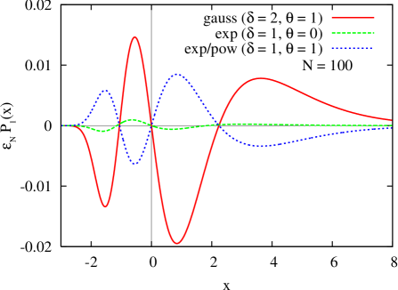
Figure 1: (Color online) First order corrections $\epsilon_{N}P_{1}(x,\gamma,\gamma^{\prime})=[\epsilon_{N}M_{1}(x,\gamma,\gamma^{\prime})]^{\prime}$ to the limit distribution density in the FTG class, $\gamma=0$, for the generalized exponential case $\mu(z)\approx 1-Be^{-Az^{\delta}}/z^{\theta}$. The different magnitudes of the shape corrections are illustrated by evaluating the amplitude $\epsilon_{N}$ at the same batch-size $N=100$. Note that while the curves marked as gauss and exp have the same shape with different prefactors, the functional form of exp/pow is slightly different.

Fig.1 displays the corrections to limit distributions for the three examples treated above (V.34,V.35,V.36) using the standardization (II.8) adopted here for theoretical reasons. The aim here is to illustrate empirical plots of the first order corrections including the amplitude $\epsilon_{N}$. One can clearly see that the fastest convergence occurs for the exponential parent distribution. Furthermore, while the functional forms for the Gaussian ($\delta=2,\,\theta=1$) and for the power law corrected exponential ($\delta=1,\,\theta=1$) are the same, the difference in the sign of the correction makes the empirical distinction apparent.

VI Unstable eigenfunctions and invariant manifolds

So far we have been concentrating on the small neighborhood of the fixed line. However, regions far away from the critical line where the space of distribution functions with respect to the RG transformation becomes more complex, are also of interest. In order to explore those regions, we should select special parent distributions. Upon the action of the RG transformation with $p>1$, the parent distributions we considered approached a fixed point along a stable eigendirection. This is the last surviving perturbation and represents the finite-size correction to the limit distribution for large batch size $N$, and is characterized by $\gamma^{\prime}\leq 0$. On the other hand, eigenvalues $\lambda=p^{\gamma^{\prime}}>1$ also exist corresponding to $\gamma^{\prime}>0$. So the question naturally arises: what happens, if we start out from a parent distribution that is close to a fixed point labeled by $\gamma$, and differs from it in an unstable eigenfunction $\psi(x;{\gamma,\gamma^{\prime}})$ with a small magnitude $\epsilon$. Initially, the distribution will move away from the fixed point by the action of the linearized RG but the evolution becomes nontrivial at later stages due to the nonlinearities present. One can nevertheless pose the question whether parent distribution belongs to the domain of attraction of a standard EVS fixed point.

By evolving a distribution containing an unstable eigendirection as a perturbation about a fixed point, an invariant unstable manifold emerges. This manifold can be determined order by order in the perturbation parameter $\epsilon$, by the successive application of the RG transformation. An ambiguity emerges, however, as to how a perturbation proportional to $\epsilon$ is introduced. This is exemplified by two natural choices of distributions (III.1,III.2), redisplayed with an eigenfunction as perturbation

$$\mu_{1}(z) =M(z+\epsilon\psi(z;\gamma,\gamma^{\prime});\gamma),$$ (VI.1a)

$$\mu_{2}(z) =M(z;\gamma)+\epsilon P(z;\gamma)\psi(z;\gamma,\gamma^{\prime}),$$ (VI.1b)

​​where $M$ is a fixed point distribution, $P$ its density, $\psi$ is given by (III.15), and $\epsilon$ is a small, but fixed, parameter. While these distributions are the same up to linear order in $\epsilon$, they generically differ in higher order terms and in their large-$z$ asymptote. Thus it matters which distribution we start with, because they will track different manifolds. More variants equivalent to linear order are also possible, but we restrict our attention to the above two types.

A problem to be considered when various linear perturbations are introduced, as in Eqs. (VI.1), is that we should have a valid (monotonic from 0 to 1) distribution for finite $\epsilon$ in some support in $z$. Since the eigenfunctions $\psi(z;\gamma,\gamma^{\prime})$ are non-monotonic in $z$, extra care should be exercised. In particular, the equivalence of the two forms in (VI.1) holds only for $|\epsilon\psi(z;\gamma,\gamma^{\prime})|\ll|z|$, but this condition is generically not fulfilled in the entire support. We circumvent the above problem by considering particular parent distributions, specifying which form in (VI.1) should be understood, and determining some allowed sets of the parameters $\epsilon,\gamma^{\prime}$. Below, we shall discuss separately the unstable invariant manifolds emanating from the three classes of fixed point distributions.

VI.1 Instability near the FTG fixed point

First we shall consider the parent of the form (VI.1a)

$$\mu(z)=\mu_{1}(z)=e^{-e^{-z-\epsilon\psi(z)}},$$ (VI.2)

where $\epsilon$ is assumed small but finite and fixed, and

$$\psi(z)=\psi(z;0,\gamma^{\prime})=\frac{1}{\gamma^{\prime 2}}\left(1+\gamma^{\prime}z-e^{\gamma^{\prime}z}\right)$$ (VI.3)

is an unstable eigenfunction with $\gamma^{\prime}>0$. It is easy to see that for $0<-\epsilon<\gamma^{\prime}$ we have a strictly increasing $\mu(z)$ for all $z$, so the support extends over the entire real axis. For sufficiently large $z$, however, in the region of importance for extreme statistics, one has $\epsilon\psi(z)\gg z$, so an expansion in $\epsilon$ is no longer legitimate and (VI.2) is not equivalent to the corresponding formula in (VI.1b) even for small $\epsilon$.

We now would like to determine whether the parent is attracted to a fixed point, and, if so, what its finite-size correction is. The associated parameters will be denoted by $\tilde{\gamma}$, labeling the attracting fixed point, and $\tilde{\gamma}^{\prime}$, specifying the eigenfunction of the final approach. These parameters can be determined by means of the relations given in Sec. V.3, namely

$$g(z) =-\ln(-\ln\mu(z))$$

$$=z+\epsilon\psi(z)\approx\frac{|\epsilon|}{\gamma^{\prime 2}}e^{\gamma^{\prime}z},$$ (VI.4a)

$$b_{N} =g^{-1}(\ln N)\approx\frac{1}{\gamma^{\prime}}\ln{\left(\frac{\gamma^{\prime 2}}{|\epsilon|}\ln N\right)},$$ (VI.4b)

$$a_{N} =\frac{1}{g^{\prime}(b_{N})}\approx\frac{\gamma^{\prime 2}}{|\epsilon|}e^{-\gamma^{\prime}b_{N}}.$$ (VI.4c)

Convergence is characterized by the effective $\gamma_{N}$ defined in (V.16), which now approaches $\tilde{\gamma}$, and by the perturbation parameter $\epsilon_{N}$ given in (V.15). We now have

$$\gamma_{N}=\frac{da_{N}}{db_{N}}=\tilde{\gamma}+\epsilon_{N}\approx-\frac{\gamma^{\prime 2}}{|\epsilon|}e^{-\gamma^{\prime}b_{N}}.$$ (VI.5)

Hence we can easily determine the indices of universality

$$\gamma_{N} \to\tilde{\gamma}=0,$$ (VI.6a)

$$\epsilon_{N} =\gamma_{N}\approx-\frac{1}{\ln N},$$ (VI.6b)

$$\tilde{\gamma}^{\prime} =0.$$ (VI.6c)

The third line follows from the slower than power decay in the second one. Note that the function $g(z)$ discussed in this subsection diverges faster than any power and, accordingly, the result (VI.6b) can be obtained as the $\delta\to\infty$ limit of (V.29).

Summarizing, if we start out from the parent (VI.2) close to the FTG fixed point, but differing from it in an unstable eigenfunction then the RG transformation drives it to the same fixed point along the eigendirection with marginal eigenvalue $1$. That is, this unstable manifold with a $\gamma^{\prime}>0$ loops back along the marginally stable one with $\tilde{\gamma}^{\prime}=0$. We illustrate this effect as follows. On Fig. 2a the initial $\gamma^{\prime}=1.5$ and $\epsilon=-0.01$ was taken, and the extreme value density of $N$ variables displayed for some increasing $N$, showing the increasing deviation from FTG. The $N$ here corresponds to the parameter $p$ of the RG transformation (II.7). Figure 2b, on the other hand, shows that for further increasing $N$ the sequence of distributions approach FTG, thus completing the loop of the invariant manifold.

The loop in function space can be further visualized by plotting the evolution of difference from the FTG limit distribution as $N$ changes (Fig.3). A feature which can be easily seen on this plot is that the initial and the final small deviations from the FTG have different functional forms corresponding to the different values of $\gamma^{\prime}$ and $\tilde{\gamma}^{\prime}$.

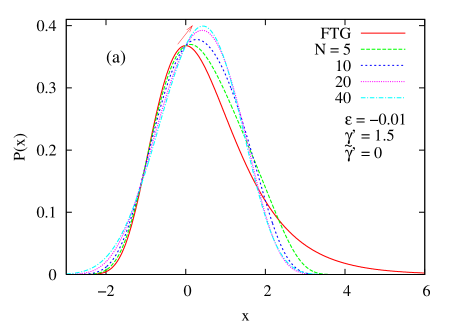
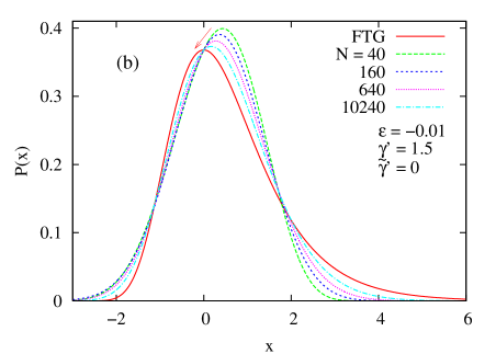
Figure 2: (Color online) Probability densities on the invariant manifold starting from the unstable parent (VI.2) with (VI.3): (a) A sequence of densities diverging from FTG. (b) A sequence of densities returning towards FTG. The arrows mark the direction of $N$ increasing. The initial $\epsilon,\gamma^{\prime}$ and final $\tilde{\gamma}^{\prime}$ parameters are indicated. Since the effective $\gamma_{N}$ tends to zero logarithmically slowly, see (VI.6b), one has to go up to relatively high $N$ to demonstrate convergence to the FTG distribution.

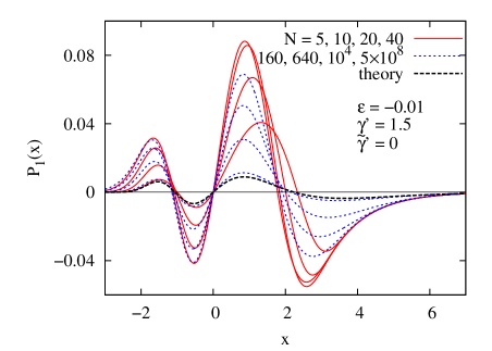
Figure 3: (Color online) The differences from FTG of the densities plotted in Fig. 2. The magnitudes of the solid red curves increase while those of the dotted blue ones decrease with $N$. It is apparent that the initial and final shape corrections have different functional form (the solid blue and dotted red curves with smallest magnitude). For illustration, the marginal correction function (“theory”) with the amplitude $\epsilon_{N}=-1/\ln N$ ($N=5\times 10^{8}$) from (VI.6b) is also displayed (dashed black line), well approximating the last dotted blue curve.

In order to demonstrate the difference of the forms (VI.1a) and (VI.1b), next we consider the same perturbation as in (VI.2) but now defined through the form (VI.1b). That is, we take the parent

$$\mu(z)=\mu_{2}(z)=e^{-e^{-z}}\left[1+\epsilon\psi(z)e^{-z}\right]\,,$$ (VI.7)

where (VI.3) is implied. To have $\mu(z)\to 1$ from below for $z\to\infty$, we should set $1>\gamma^{\prime}>0$ and $\epsilon>0$. Note that formula (VI.7) would yield negative $\mu(z)$ for large negative arguments, but $\mu(z)$ becomes positive for smaller negative arguments, and a sufficiently small $\epsilon$ ensures that thenceforth $\mu(z)$ is strictly increasing. Thus if we discard the region of negativity from the support then the function so obtained becomes a legitimate integrated probability distribution. For small enough $\epsilon$ it is obviously an unstable direction, and thus the source of an invariant manifold after RG transformations. Its large $z$ behavior can be characterized by the function $g(z)$ in (V.7) as

$$\begin{split}g(z)&=-\ln(-\ln\mu(z))\\ &\approx(1-\gamma^{\prime})z+\ln\frac{\gamma^{\prime 2}}{\epsilon}+\gamma^{\prime}ze^{-\gamma^{\prime}z}\\ &\ \ \ -\frac{\epsilon}{2\gamma^{\prime 2}}e^{-(1-\gamma^{\prime})z},\end{split}$$ (VI.8)

where we kept competing exponential terms. Hence, according to the procedure set forth in Sec. V.3, we obtain

$$b_{N}=g^{-1}(\ln N)\approx\frac{\ln\left(\epsilon N/\gamma^{\prime 2}\right)}{1-\gamma^{\prime}},$$ (VI.9)

and

$$\begin{split}\gamma_{N}&=-\frac{g^{\prime\prime}(b_{N})}{g^{\prime 2}(b_{N})}\\ &\approx\left\{\begin{array}[]{lr}c\,N^{-\frac{\gamma^{\prime}}{1-\gamma^{\prime}}}\ln N,&0<\gamma^{\prime}\leq 1/2,\\ \dfrac{1}{2N},&1/2<\gamma^{\prime}<1,\end{array}\right.\end{split}$$ (VI.10)

where the constant $c$ depends on $\epsilon$ and $\gamma^{\prime}$. Since $\gamma_{N}\to\tilde{\gamma}=0$, again the FTG fixed point is approached. Thus we have $\epsilon_{N}=\gamma_{N}$, whose decay is characterized by the index

$$\tilde{\gamma}^{\prime}=\left\{\begin{array}[]{lr}-\dfrac{\gamma^{\prime}}{1-\gamma^{\prime}},&0<\gamma^{\prime}\leq 1/2,\\ -1,&1/2\leq\gamma^{\prime}<1.\end{array}\right.$$ (VI.11)

Hence a nonmarginal asymptotic index, $\tilde{\gamma}^{\prime}<0$, is obtained, which characterizes the last surviving eigenfunction. This should be contrasted with the previously discussed case of (VI.2), where independently of the initial $\gamma^{\prime}$ we had $\tilde{\gamma}^{\prime}=0$ as shown in (VI.6c). That demonstrates the inequivalence of the distributions with unstable perturbations, (VI.1a) and (VI.1b) in the sense that depending on whether we apply the perturbation additively or in the argument, different limiting properties emerge. The unstable manifold generated from (VI.7) is illustrated on Figs. 4.

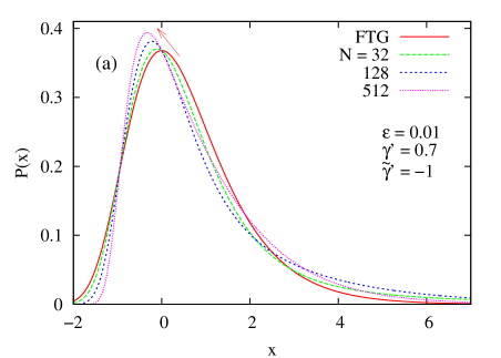
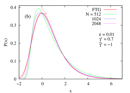
Figure 4: (Color online) Probability densities on the invariant manifold starting from the unstable parent (VI.7) with (VI.3): (a) A sequence of densities diverging from FTG. (b) A sequence of densities returning towards FTG. Arrows mark the direction of increasing $N$. The convergence to FTG is markedly faster than that along the marginal eigendirection in Fig. 2.

VI.2 Instability near the FTF fixed point

Consider the parent of the type (VI.1a)

$$\mu(z)=\mu_{1}(z)=e^{-(1+\gamma z+\epsilon\gamma\psi(z))^{-1/\gamma}},$$ (VI.12)

where $\psi(z)$ abbreviates $\psi(z;\gamma,\gamma^{\prime})$ as given by (III.15) and $\gamma,\gamma^{\prime}>0$. This is a legitimate integrated distribution in $[-1/\gamma,\infty)$ if $\gamma^{\prime}>-\epsilon>0$. Note that $\mu(z)$ has a positive value at the lower border $-1/\gamma$, below it we define $\mu(z)$ to be zero.

We again denote by $\tilde{\gamma},\tilde{\gamma}^{\prime}$ the characteristic parameters for the above parent. The procedure for calculating them was described in Sec. V.3. We now have

$$g(z) =-\ln(-\ln\mu(z))$$

$$=\frac{1}{\gamma}\ln(1+\gamma z+\gamma\epsilon\psi(z)),$$ (VI.13)

$$e^{\gamma g(b_{N})} =1+\gamma b_{N}+\gamma\epsilon\psi(b_{N})=N^{\gamma},$$ (VI.14)

$$a_{N} =\frac{1}{g^{\prime}(b_{N})}=\frac{1+\gamma b_{N}+\gamma\epsilon\psi(b_{N})}{1+\epsilon\psi^{\prime}(b_{N})}.$$ (VI.15)

Expanding the above formula in $y_{N}=1+\gamma b_{N}$, using (V.16) and the expression for $\psi(z)$ in (III.15), we obtain

$$\gamma_{N} =\frac{da_{N}}{db_{N}}=\gamma\frac{da_{N}}{dy_{N}}$$

$$\approx\frac{\gamma^{2}}{\gamma^{\prime}+\gamma}+\frac{\gamma-\gamma^{\prime}}{\gamma+\gamma^{\prime}}\gamma^{\prime}\left(\frac{\gamma^{\prime}}{|\epsilon|}-1\right)y_{N}^{-\gamma^{\prime}/\gamma}$$

$$+O(y_{N}^{-\gamma^{\prime}/\gamma-1})+O(y_{N}^{-2\gamma^{\prime}/\gamma}).$$ (VI.16)

The large-$N$ limit determines the index of the attracting fixed point

$$\tilde{\gamma}=\frac{\gamma^{2}}{\gamma^{\prime}+\gamma}.$$ (VI.17)

This is just the asymptotic exponent in $b_{N}\propto N^{\tilde{\gamma}}$, which also can be obtained from (VI.14) and the dominant term in (III.15). Next, we have to determine the leading power of $N$ in

$$\epsilon_{N}=\gamma_{N}-\tilde{\gamma}\propto N^{\tilde{\gamma}^{\prime}}.$$ (VI.18)

One should distinguish the case $\gamma^{\prime}=\gamma$, the amplitude of the term $y_{N}^{-\gamma^{\prime}/\gamma}$ vanishes in (VI.16), and the leading correction becomes $y_{N}^{-2}$. Using $b_{N}\propto y_{N}$ in (VI.16) we finally obtain

$$\tilde{\gamma}^{\prime}=\left\{\begin{array}[]{lr}-\dfrac{\gamma\gamma^{\prime}}{\gamma^{\prime}+\gamma},&\gamma^{\prime}\neq\gamma,\\ -\gamma^{\prime},&\gamma^{\prime}=\gamma.\end{array}\right.$$ (VI.19)

We illustrate the above described invariant manifold on Fig. 5, with starting parameters $\gamma=1.5,\gamma^{\prime}=3$ resulting in final ones $\tilde{\gamma}=0.5,\tilde{\gamma}^{\prime}=-1$.

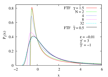
Figure 5: (Color online) Sequence of densities on an invariant manifold of the form (VI.12), with increasing $N$ tracking the RG trajectory. In variance with the FTG case, the starting and final distributions are different here. Note that while convergence to the latter is well demonstrated, the maximum decreases to below the limit before the final approach. This is related to the fact that the effective $\gamma_{N}$ in (VI.16) approaches the limit from below.

In order to demonstrate the inequivalence of (VI.1a) and (VI.1b) also in the FTF case, we consider the example

$$\mu(z)=\mu_{2}(z)=e^{-(1+\gamma z)^{-{1}/{\gamma}}}\left[1+\epsilon\psi(z)(1+\gamma z)^{-{1}/{\gamma}-1}\right].$$ (VI.20)

Given the form of $\psi$ in (III.15), the decay of the perturbation for large $z$ requires $\gamma^{\prime}<1$. It is easy to see that near the lower border of the support of the unperturbed limit distribution, in some interval for $z<0$, this function is negative. Then for increasing argument it becomes positive, and for not too large $\epsilon$ it remains monotonic thereafter. Since the EVS limit behavior depends on the large-$z$ asymptote, we simply discard the region of negativity from the support, thus we wind up with a legitimate parent distribution, given by (VI.20) whenever it is non-negative. We keep only the asymptotic terms necessary to determine the final indices

$$\begin{split}g(z)&=-\ln(-\ln\mu(z))\\ &\approx\frac{1-\gamma^{\prime}}{\gamma}\ln(1+\gamma z)+c_{1}\\ &+c_{2}(1+\gamma z)^{-\gamma^{\prime}/\gamma}+c_{3}(1+\gamma z)^{-(1-\gamma^{\prime})/\gamma},\end{split}$$ (VI.21)

where the constants $c_{j}$ depend on the parameters $\epsilon,\gamma,\gamma^{\prime}$. Repeating the steps of the procedure set forth in Sec. V.3, we find

$$\tilde{\gamma} =\dfrac{\gamma}{1-\gamma^{\prime}},$$ (VI.22a)

$$\tilde{\gamma}^{\prime} =\left\{\begin{array}[]{lr}-\dfrac{\gamma^{\prime}}{1-\gamma^{\prime}},&0\leq\gamma^{\prime}\leq 1/2,\\ -1,&1/2\leq\gamma^{\prime}<1.\end{array}\right.$$ (VI.22d)

On Fig. 6 we illustrate this case with $\epsilon=0.01,\gamma=0.5,\gamma^{\prime}=2/3$. The asymptotic indices can be read off from Eq, (VI.22) as $\tilde{\gamma}=1.5$ and $\tilde{\gamma}^{\prime}=-1$.

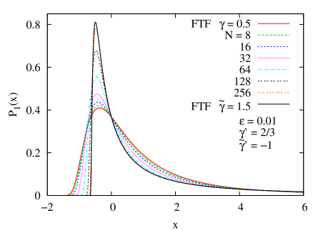
Figure 6: (Color online) Sequence of densities on an invariant manifold starting out from (VI.20), where increasing $N$ follows the RG trajectory. Again, the starting and final distributions are different, but in contrast with the case (VI.12), illustrated on Fig. 5, the final $\tilde{\gamma}$ is larger than the initial $\gamma$.

Summarizing, the parent with perturbed argument (VI.12), representing an unstable function near an FTF fixed point with $\gamma>0$ and having an instability parameter $\gamma^{\prime}>0$, will eventually be attracted to another FTF limit distribution with $\tilde{\gamma}$ as in (VI.17). The final approach happens along the stable manifold with parameter $\tilde{\gamma}^{\prime}$ as in (VI.19). In contrast, if we additively perturb the fixed point and take for the parent (VI.20), we get a different set of indices $\tilde{\gamma},\tilde{\gamma}^{\prime}$, as given in (VI.22).

VI.3 Instability near the FTW fixed point

In the FTW case, the two types of parent distributions, (VI.1a) and (VI.1b) have the same formulas as for the FTF class, (VI.12) and (VI.20), respectively, but we have $\gamma<0$ for FTW. As we shall see, however, the properties of the FTW case cannot be obtained by trivially changing the sign of $\gamma$ in the FTF results.

Consider first the parent of the form (VI.12), with $\gamma<0$. For our present purposes it suffices to mention that for $\gamma^{\prime}>-\epsilon>0$ monotonicity holds, furthermore, the upper limit of the support $z^{\ast}$, where $g(z)$ diverges, is some value below $1/|\gamma|$. Near $z^{\ast}$ the argument of the log in (VI.13),

$$\phi(z)=e^{\gamma g(z)},$$ (VI.23)

is analytic, whence we can determine the indices of universality following Sec. V.3. We have to determine the effective index

$$\gamma_{N}=\gamma+\epsilon_{N}=-\frac{g^{\prime\prime}(b_{N})}{g^{\prime 2}(b_{N})}=\gamma-\frac{\gamma\phi(b_{N})\phi^{\prime\prime}(b_{N})}{\phi^{\prime 2}(b_{N})}.$$ (VI.24)

Now the $N\to\infty$ limit of the effective $\gamma_{N}$ gives $\tilde{\gamma}$, while the decay of $\epsilon_{N}$ provides the index $\tilde{\gamma}^{\prime}$. They can be obtained by noting that from (VI.14) we have $\phi(b_{N})=N^{\gamma}$ and higher derivatives of $\phi(b_{N})$ go to constants. Thus the limit of (VI.24) is

$$\tilde{\gamma}=\gamma,$$ (VI.25)

and the exponent of convergence of $\epsilon_{N}$ is equally

$$\tilde{\gamma}^{\prime}=\gamma.$$ (VI.26)

Thus, we found that the unstable manifold returns to the same fixed point along the stable manifold whose stability parameter $\tilde{\gamma}^{\prime}$ coincides with the fixed point parameter, irrespective of the initial value of the instability parameter $\gamma^{\prime}$.

Turning to the case of the additively perturbed distribution, we use (VI.20) with $\gamma<0$. If $1>-\gamma>\gamma^{\prime}>0$ then, for not too large $\epsilon>0$, one has the same upper limit of support $z^{\ast}=-1/\gamma$ as in the unperturbed case, and

$$\begin{split}g(z)&=-\ln(-\ln\mu(z))\\ &\approx\frac{1+\gamma}{\gamma}\ln(1+\gamma z)+d_{1}\\ &+d_{2}(1+\gamma z)^{\gamma^{\prime}/\gamma+1}+d_{3}(1+\gamma z)^{-(1+\gamma)/\gamma},\end{split}$$ (VI.27)

where $d_{j}$ are constants. We calculate again the effective $\gamma_{N}$ according to Sec. V.3, and wind up with the following final indices

$$\tilde{\gamma} =\dfrac{\gamma}{1+\gamma},$$ (VI.28a)

$$\tilde{\gamma}^{\prime} =\max\left\{\frac{\gamma+\gamma^{\prime}}{1+\gamma},-1\right\}.$$ (VI.28b)

Comparison of (VI.28) with (VI.25,VI.26) demonstrates once more that the asymptotic properties strongly depend on the way the unstable perturbation is applied. Plots of the evolution of distributions as $N$ increases for initial states with $\gamma<0<\gamma^{\prime}$ are qualitatively similar to previous figures, therefore we do not display them.

VI.4 Unstable manifolds in function space

The results above on the unstable manifolds emanating from the eigendirections of the form (VI.1a) are graphically represented in function space on Fig. 7. If we start out from a parent distribution near the fixed point with $\gamma$, in the direction of the unstable eigenfunction with $\gamma^{\prime}>0$, then upon the action of the RG transformation the distribution function moves on an unstable manifold. For $\gamma\leq 0$, the FTW case, the unstable manifold loops back towards the same fixed point, whose neighborhood it started out from. On the other hand, in the FTF case, $\gamma>0$, the RG trajectory will wind up in the fixed point with $\tilde{\gamma}<\gamma$, as given in (VI.17), falling between the starting and the FTG fixed points. The characteristic parameter of the stability is $\tilde{\gamma}^{\prime}=\gamma$ for the case $\gamma\leq 0$, whereas for the FTF class, $\gamma>0$, the parameter of the stable eigendirection is given by Eq. (VI.19).

\psfrag{c}{$\gamma>0$}\psfrag{b}{$\tilde{\gamma}(<\gamma)$}\psfrag{f}{$\gamma^{\prime}\!>\!0$}\psfrag{a}{$\tilde{\gamma}^{\prime}=\tilde{\gamma}=\gamma=0$}\psfrag{g}{$\tilde{\gamma}^{\prime}\!\!<\!0$}\psfrag{d}{$\gamma$}\psfrag{e}{$\tilde{\gamma}^{\prime}=\tilde{\gamma}=\gamma\!<\!0$}\psfrag{ww}{FTW}\psfrag{gg}{FTG}\psfrag{ff}{FTF}\includegraphics[width=236.15796pt]{rg.eps}

Figure 7: Illustration of the invariant manifolds of various fixed points in the space of probability distributions. Starting distributions near a fixed point with some $\gamma$, differing from it by an eigenfunction with a parameter $\gamma^{\prime}>0$, with the definition in (VI.1a). The straight line is the $\gamma$ axis and the directed curves represent RG transformation flows. Each flow ends up in a fixed point with $\tilde{\gamma}$ along a stable direction characterized by the finite-size index $\tilde{\gamma}^{\prime}\leq 0$. The approach to the FTG fixed point is along the marginal direction $\tilde{\gamma}^{\prime}=0$, which corresponds to a small perturbation on the fixed line, as discussed in Sec. III.3.

The invariant manifolds starting from unstable distributions of the form (VI.1b) are illustrated on Fig. 8. For the cases $\gamma\neq 0$ the RG trajectory will wind up in the fixed point with a different $\tilde{\gamma}$, farther from the origin. This can be understood from the fact that the additive perturbation in (VI.1b) slows down the asymptote of the distribution, while such effect is not present if the perturbation is in the argument like in (VI.1a). The characteristic parameter of the asymptotic stability is $\tilde{\gamma}^{\prime}<0$ in all cases.

\psfrag{b}{$\gamma>0$}\psfrag{c}{$\tilde{\gamma}(>\gamma)$}\psfrag{f}{$\gamma^{\prime}>0$}\psfrag{h}{$\gamma^{\prime}<0$}\psfrag{a}{$\tilde{\gamma}=\gamma=0$}\psfrag{g}{$\gamma<0$}\psfrag{d}{$\gamma$}\psfrag{e}{$\tilde{\gamma}(<\gamma)$}\psfrag{ww}{FTW}\psfrag{gg}{FTG}\psfrag{ff}{FTF}\includegraphics[width=236.15796pt]{rg2.eps}

Figure 8: Illustration of the invariant manifolds from starting distributions with $\gamma^{\prime}>0$ in the definition (VI.1b). Each flow converges to a fixed point with $\tilde{\gamma}$ along a stable direction characterized by a finite-size index $\tilde{\gamma}^{\prime}<0$.

Note that on the fixed line there is a symmetry between a $\gamma>0$ and its negation, i.e., the FTF and FTW cases. In particular, in the FTF case with a $\gamma>0$, the variable $1+\gamma x$ has the same distribution as in the FTW case, with the parameter $-\gamma$, the variable $1/(1-\gamma x)$ has. Nevertheless, this symmetry does not manifest itself for the invariant manifolds. On the one hand, in (VI.1a) the symmetry is broken, since $\psi$ is added to the variable itself in the argument. This is also responsible for the effect that in the FTF case the decay of the limit distribution is stronger than that of the parent. On the other hand, for the additively perturbed distributions of the form (VI.1b) there is a qualitative symmetry, in that the RG trajectory loops back to the fixed line farther from the origin for both signs of the starting $\gamma$. The particular values of the final $\tilde{\gamma},\tilde{\gamma}^{\prime}$ indices, as given by (VI.22) and (VI.28), however, do not exhibit the sign flip symmetry of the fixed line.

VII Conclusion and outlook

We have shown how finite-size corrections to EVS limit distributions can be derived by borrowing ideas and terminology from the RG theory. The corrections in shape and amplitude emerged from the action of the RG transformation on the function space associated with the close neighborhood of the fixed line of limit distributions. This RG approach provided the classification of the first-order corrections and, furthermore, it also helped to establish the connection to parent distributions, thus making the results practically useful. A remarkable feature of the RG theory is that the study of the linear neighborhood of the fixed line reveals orbits – invariant manifolds – of the RG transformation which first diverge and later return to the same or to a different point on the fixed line.

There are several problems in EVS where the RG approach developed here may be of interest. Within the theory of EVS of i.i.d. variables, the RG theory should be instrumental in developing a compact treatment of the finite-size corrections for order statistics in general, among them for the 2nd, 3rd, etc. maxima, as well as for their various joint statistics. Furthermore, higher order corrections are also of interest from the empirical viewpoint, especially in the case of the logarithmically slow convergence.

The next level of difficulty is met when trying to investigate the problem of weakly correlated variables (a nontrivial example is the stationary sequence of Gaussian variables with correlation decaying as a power law) where the EVS limit distribution of the maximum is known to be FTG Berman (1964)). There the question arises naturally, whether the finite-size corrections elucidated in this paper remain valid for families of sufficiently weakly correlated variables. There is ground to believe that the finite-size corrections may be the same Györgyi et al. (2007) but further studies are needed to clarify the matter.

Finally, the extension of the RG approach to calculate the EVS of strongly correlated systems appears to be a real challenge. We are aware of only one work Schehr and Le Doussal (2009) where the so called real-space renormalization group was developed for obtaining EVS of random walk type processes. The results are restricted presently to the limit distributions for these processes. It would be certainly interesting to extend the method to find the finite-size corrections and compare with the phenomenological approaches Györgyi et al. (2008) since some of them suggests that the shape corrections can be calculated from the limit distributions.