Electron spin relaxation in graphene from a microscopic approach: Role of electron-electron interaction

Abstract

Electron spin relaxation in graphene on a substrate is investigated from the microscopic kinetic spin Bloch equation approach. All the relevant scatterings, such as the electron-impurity, electron–acoustic-phonon, electron–optical-phonon, electron–remote-interfacial-phonon, as well as electron-electron Coulomb scatterings, are explicitly included. Our study concentrates on clean intrinsic graphene, where the spin-orbit coupling from the adatoms can be neglected. We discuss the effect of the electron-electron Coulomb interaction on spin relaxation under various conditions. It is shown that the electron-electron Coulomb scattering plays an important role in spin relaxation at high temperature. We also find a significant increase of the spin relaxation time for high spin polarization even at room temperature, which is due to the Coulomb Hartree-Fock contribution-induced effective longitudinal magnetic field. It is also discovered that the spin relaxation time increases with the in-plane electric field due to the hot-electron effect, which is different from the non-monotonic behavior in semiconductors. Moreover, we show that the electron-electron Coulomb scattering in graphene is not strong enough to establish the steady-state hot-electron distribution widely used in the literature and an alternative approximate one is proposed based on our computation.

I Introduction

Graphene, as a strictly two-dimensional material, has revealed a cornucopia of new physics and potential applications, and thus has attracted much attention in recent years.Geim_07 This material is also important for spintronics since the spin relaxation time (SRT) in intrinsic graphene is expected to be very long. The underlying reason is the low hyperfine interaction of the spin with the carbon nuclei (natural carbon only contains 1% ¹³C with spin) and the weak spin-orbit coupling (SOC) due to the low atomic number.Loss_hyper ; Kane_SOC ; Hernando_06 ; Min ; Fang_07 ; Fabian_SOC

The study of spin relaxation in graphene is still in the initial stage. Some investigations have been performed on the spin relaxation due to the D’yakonov-Perel’ (DP) mechanismDyakonov in graphene.Fabian_SR ; Hernando_07 ; Hernando_09 This relaxation mechanism is from the joint effects of the momentum scattering and the momentum-dependent spin-orbit field (inhomogeneous broadeningWu_01 ; Wu_rev ). However, the previous investigations are all in the framework of single-particle approach, thus the electron-electron Coulomb scattering, which has been demonstrated to be very important for the spin relaxation in bulk and low-dimensional semiconductor systems,Wu_01 ; Wu_rev ; Zhou_PRB_07 ; Jiang_bulk_09 ; highP ; wu-exp-hP ; tobias ; Zheng_exp ; hot-e ; multi ; Ivchenko ; Leyland ; Ji was not included. Understanding the effect of the electron-electron Coulomb scattering on spin relaxation in graphene is an important problem. In addition, the Coulomb Hartree-Fock (HF) term acts as an effective longitudinal magnetic field, and hence can increase the SRT by more than one order of magnitude for high initial spin polarization in semiconductors at low temperature.highP ; wu-exp-hP ; tobias ; Zheng_exp ; Jiang_bulk_09 Whether it is still valid in graphene remains unchecked. Also, in semiconductors the spin relaxation can be effectively manipulated by the high in-plane electric field.hot-e ; multi ; Jiang_bulk_09 How the in-plane electric field affects the spin relaxation in graphene is also unclear. In the present paper, we investigate the spin relaxation in graphene from the microscopic kinetic spin Bloch equation (KSBE) approach,Wu_rev which has achieved much success in the study of the spin dynamics in semiconductors. Via this approach, we can explicitly include all the relevant scatterings, especially the electron-electron Coulomb scattering, and understand the physics raised above.

It is also noted that there is a significant discrepancy between the existing theories and the recent spin transport experiments.Tombros_07 ; Tombros_08 ; Popinciuc ; Jozsa_09 These experiments reported the SRTs of only about $150$ ps, at least one order of magnitude shorter than the lowest value obtained in the theory.Fabian_SR ; Hernando_07 ; Hernando_09 This suggests that the SRTs obtained in the recent experiments are likely to be limited by an extrinsic mechanisms, e.g., the local spin-orbit field from the adatoms.Fabian_SR ; Hernando_09 ; Castro_imp In this paper we concentrate on the relatively cleaner graphene samples by choosing low impurity densities which give a mobility higher than the values in the latest experiments, so that the effect of the adatoms can be neglected.

This paper is organized as follows. In Sec. II, we present the model and introduce the KSBEs. Then in Sec. IIIA, we discuss the effect of the electron-electron Coulomb interaction on spin relaxation at various temperature, electron density, initial spin polarization and in-plane electric field. We discuss the hot-electron distribution function in the steady state in Sec. IIIB. Finally, we summarize in Sec. IV.

II Model and KSBEs

We start our investigation from a graphene layer on a SiO₂ substrate. The $z$-axis is set perpendicular to the graphene plane. A uniform electric field ${\bf E}_{\|}$ and a uniform magnetic field ${\bf B}$ are applied along the $x$- and $y$-axes respectively (the Voigt configuration). Without the SOC and the external field, the band structure of graphene near the $K$ and $K^{\prime}$ points can be described by the effective Hamiltonian ($\hbar\equiv 1$)DiVincenzo

$$H_{0}^{\mu}=v_{\rm F}(\mu\sigma_{x}k_{x}+\sigma_{y}k_{y}).$$ (1)

Here $\mu=1(-1)$ for $K(K^{\prime})$ valleys; $v_{\rm F}$ is the Fermi velocity; ${\bf k}$ represents the two-dimensional wave vector relative to $K(K^{\prime})$ points; $\bm{\sigma}$ is the Pauli matrix in the pseudospin space formed by the A and B sublattices of the honeycomb lattice. The eigenvalues of $H_{0}^{\mu}$ are $\epsilon_{\mu\nu{\bf k}}=\nu v_{\rm F}|{\bf k}|$ with $\nu=1(-1)$ for electron (hole) band. The corresponding eigenstates are $\psi_{{\bf k}}^{\mu\nu}=1/\sqrt{2}(\mu\nu e^{-i\mu\theta_{\bf k}},1)^{\rm T}$ with $\theta_{\bf k}$ representing the polar angle of ${\bf k}$. We introduce an orthogonal and complete basis set $\Psi_{{\bf k}s}^{\mu\nu}=\psi_{{\bf k}}^{\mu\nu}\otimes\chi_{s}$ with $\chi_{s}$ being the eigenstate of the spin Pauli matrix $s_{z}$. In this basis set, the total Hamiltonian including the SOC can be written asFabian_SR ; correct

$${H}_{\mathrm{eff}} = \sum_{{\mu}\nu{\bf k}ss^{\prime}}\big{[}(\epsilon_{\mu\nu{\bf k}}-\lambda_{\rm I}-e{\bf E}_{\|}\cdot{\bf R})\delta_{ss^{\prime}}$$ (2)

$$+(g\mu_{B}{\bf B}+\nu\bm{\Omega}_{\bf k})\cdot\mathbf{s}_{ss^{\prime}}\big{]}{c^{{\mu}\nu}_{{\bf k}s}}^{\dagger}c^{{\mu}\nu}_{{\bf k}s^{\prime}}+{H}_{\rm int}.$$

where ${\bf R}=(x,y)$ is the electron position. $c^{{\mu}\nu}_{{\bf k}s}$ (${c^{{\mu}\nu}_{{\bf k}s}}^{\dagger}$) is the annihilation (creation) operator of the state $\Psi_{{\bf k}s}^{\mu\nu}$. $e$ is the electron charge ($e>0$). $g=2$ is the effective Landé factor. The intrinsic SOC coefficient $\lambda_{\rm I}=0.012$ meV is from the recent first-principle calculation.Fabian_SOC From Eq. (2), it is seen that the intrinsic SOC only induces a shift of the energy spectrum of graphene. $\bm{\Omega}_{\bf k}$ denotes the effective magnetic field due to the Rashba SOC, which readsFabian_SR

$$\bm{\Omega}_{\bf k}=\alpha_{\rm R}(-\sin\theta_{\bf k},\cos\theta_{\bf k},0)$$ (3)

with $\alpha_{\rm R}=\zeta E_{z}$. The recent first-principle calculation gives $\zeta=0.005$ meV$\cdot$nm/V.Fabian_SOC The longitudinal electric field $E_{z}$ originates from the gate voltage and chemical doping. Here we choose a typical value in experiment $E_{z}=300$ kV/cm.Novoselov_Science ; Ez_sub It is noted that $\bm{\Omega}_{\bf k}$ depends on the direction of ${\bf k}$ only, but is independent on the magnitude of ${\bf k}$. Therefore the inhomogeneous broadening induced by the SOC does not change with the variation of temperature and electron density. This makes the temperature and electron-density dependences of the SRT in graphene very different from those in semiconductors.Wu_rev The interaction Hamiltonian $H_{\rm int}$ consists of the electron-impurity, electron-phonon as well as electron-electron Coulomb interactions. Their expressions are given in the appendix. In the derivation of Eq. (2), $|\epsilon_{\mu\nu{\bf k}}|\gg\alpha_{\rm R}+\lambda_{\rm I}$ is assumed and thus the terms between the electron and hole bands are neglected. This approximation is valid when the Fermi energy $E_{\rm F}$ is much larger than $0.03$ meV,Fabian_SOC ; Fabian_SR which is usually fulfilled in gated or doped graphene. In our calculation, we restrict ourselves to the $n$-doped case (i.e., $E_{\rm F}\gg k_{\rm B}T$).

By using the nonequilibrium Green function method,Haug_1998 the KSBEs can be constructed as:Wu_rev

$$\partial_{t}\hat{\rho}_{{\mu}{\bf k}}=\left.\partial_{t}\hat{\rho}_{{\mu}{\bf k}}\right|_{\rm coh}+\left.\partial_{t}\hat{\rho}_{{\mu}{\bf k}}\right|_{\rm drift}+\left.\partial_{t}\hat{\rho}_{{\mu}{\bf k}}\right|_{\rm scat},$$ (4)

where $\hat{\rho}_{{\mu}\bf k}$ represent the density matrices of electron with the relative momentum ${\bf k}$ in valley ${\mu}$, whose diagonal terms $\rho_{\mu{\bf k},ss}\equiv f_{{\mu}{\bf k}s}$ ($s=\pm\frac{1}{2}$) represent the electron distribution functions and off-diagonal ones $\rho_{\mu{\bf k},\frac{1}{2}\,{-}\frac{1}{2}}=\rho_{\mu{\bf k},{-}\frac{1}{2}\,\frac{1}{2}}^{\ast}$ describe the spin coherence. The coherent term is given by

$$\left.\partial_{t}\hat{\rho}_{{\mu}{\bf k}}\right|_{\rm coh}=-i\left[(g\mu_{B}{\bf B}+\bm{\Omega}_{\bf k})\cdot\hat{\bf s}+\hat{\Sigma}^{\rm HF}_{\mu{\bf k}},\;\;\hat{\rho}_{{\mu}{\bf k}}\right],$$ (5)

in which $[A,B]\equiv AB-BA$ is the commutator; $\hat{\Sigma}^{\mathrm{HF}}_{\mu{\bf k}}=-\sum_{{\bf k}^{\prime}}V^{\mu 11}_{{\bf k},{\bf k}^{\prime}}I_{{\bf k}{\bf k}^{\prime}}\hat{\rho}_{{\mu}{\bf k}^{\prime}}$ is the effective magnetic field from the Coulomb HF contribution.highP The drift term can be written ashot-e

$$\left.\partial_{t}\hat{\rho}_{{\mu}{\bf k}}\right|_{\rm drift}=e{\bf E}_{\|}\cdot\mbox{\boldmath$\nabla$\unboldmath}_{\bf k}\hat{\rho}_{\mu{\bf k}},$$ (6)

The scattering term $\partial_{t}\hat{\rho}_{{\mu}{\bf k}}|_{\rm scat}$ consists of the electron-impurity, electron–acoustic (AC)-phonon, electron–optical (OP)-phonon, electron–remote-interfacial (RI)-phonon as well as electron-electron Coulomb scatterings. These scattering terms are

$$\left.\partial_{t}\hat{\rho}_{{\mu}{\bf k}}\right|_{\rm ei} = -\pi N_{i}\sum_{{\bf k}^{\prime}}|U^{\mu 1}_{{\bf k},{\bf k}^{\prime}}|^{2}I_{{\bf k}{\bf k}^{\prime}}\delta(\varepsilon_{{\mu}{\bf k}^{\prime}}-\varepsilon_{{\mu}{\bf k}})\left(\hat{\rho}^{>}_{\mu{\bf k}^{\prime}}\hat{\rho}^{<}_{\mu{\bf k}}-\hat{\rho}^{<}_{\mu{\bf k}^{\prime}}\hat{\rho}^{>}_{\mu{\bf k}}\right)+{\rm H.c.},$$ (7)

$$\left.\partial_{t}\hat{\rho}_{{\mu}{\bf k}}\right|_{\rm ep} = -\pi\sum_{\mu^{\prime}{\bf k}^{\prime}\lambda,\pm}|M^{\lambda}_{\mu{\bf k},\mu^{\prime}{\bf k}^{\prime}}|^{2}\delta(\varepsilon_{{\mu^{\prime}}{\bf k}^{\prime}}-\varepsilon_{{\mu}{\bf k}}\pm\omega^{\lambda}_{{\bf k}-{\bf k}^{\prime}})\left(N^{\pm}_{\lambda,{\bf k}-{\bf k}^{\prime}}\hat{\rho}^{>}_{\mu^{\prime}{\bf k}^{\prime}}\hat{\rho}^{<}_{\mu{\bf k}}-N^{\mp}_{\lambda,{\bf k}-{\bf k}^{\prime}}\hat{\rho}^{<}_{\mu^{\prime}{\bf k}^{\prime}}\hat{\rho}^{>}_{\mu{\bf k}}\right)+{\rm H.c.},$$ (8)

$$\left.\partial_{t}\hat{\rho}_{{\mu}{\bf k}}\right|_{\rm ee} = -\pi\sum_{\mu^{\prime}{\bf k}^{\prime}{\bf k}^{\prime\prime}}|V^{\mu 11}_{{\bf k},{\bf k}^{\prime}}|^{2}I_{{\bf k}{\bf k}^{\prime}}I_{{\bf k}^{\prime\prime}\mathtt{{\bf k}^{\prime\prime}{-}{\bf k}{+}{\bf k}^{\prime}}}\delta(\varepsilon_{{\mu}{\bf k}^{\prime}}{-}\varepsilon_{{\mu}{\bf k}}{+}\varepsilon_{{\mu}^{\prime}{\bf k}^{\prime\prime}}{-}\varepsilon_{\mathtt{\mu^{\prime}{\bf k}^{\prime\prime}-{\bf k}+{\bf k}^{\prime}}})\Big{[}{\rm Tr}\left(\hat{\rho}^{<}_{\mu^{\prime}{\bf k}^{\prime\prime}{-}{\bf k}{+}{\bf k}^{\prime}}\hat{\rho}^{>}_{\mu^{\prime}{\bf k}^{\prime\prime}}\right)\hat{\rho}^{>}_{\mu{\bf k}^{\prime}}\hat{\rho}^{<}_{\mu{\bf k}}$$ (9)

$$\mbox{}-{\rm Tr}\left(\hat{\rho}^{>}_{\mu^{\prime}{\bf k}^{\prime\prime}{-}{\bf k}{+}{\bf k}^{\prime}}\hat{\rho}^{<}_{\mu^{\prime}{\bf k}^{\prime\prime}}\right)\hat{\rho}^{<}_{\mu{\bf k}^{\prime}}\hat{\rho}^{>}_{\mu{\bf k}}\Big{]}+{\rm H.c.}.$$

In these equations, $\varepsilon_{{\mu}{\bf k}}\equiv\epsilon_{\mu\nu=1{\bf k}}=v_{\rm F}|{\bf k}|$,linear $\hat{\rho}^{>}_{{\mu}{\bf k}}\equiv 1-\hat{\rho}_{{\mu}{\bf k}}$, $\hat{\rho}^{<}_{{\mu}{\bf k}}\equiv\hat{\rho}_{{\mu}{\bf k}}$; $\omega^{\lambda}_{\bf q}$ denotes the phonon energy spectrum; $N_{\lambda{\bf q}}^{\pm}=N_{\lambda{\bf q}}+\frac{1}{2}\pm\frac{1}{2}$ with $N_{\lambda{\bf q}}$ representing the phonon number at lattice temperature. The form factor $I_{{\bf k}{\bf k}-{\bf q}}=|{\psi_{{\bf k}}^{\mu 1}}^{\dagger}\psi_{{\bf k}-{\bf q}}^{\mu 1}|^{2}=\frac{1}{2}[1+\cos(\theta_{\bf k}-\theta_{{\bf k}-{\bf q}})]$. The matrix elements $U^{\mu 1}_{{\bf k},{\bf k}^{\prime}}$, $V^{\mu 11}_{{\bf k},{\bf k}^{\prime}}$ and $M^{\lambda}_{\mu{\bf k},\mu^{\prime}{\bf k}^{\prime}}$ are given in the appendix.

III Results

The KSBEs with all the scatterings explicitly included can be solved self-consistently following the numerical scheme similar to that in semiconductors, detailed in the appendix of Ref. hot-e, . Then one can obtain the temporal evolution of the electron density matrix. The SRT $T_{1}$ and ensemble spin dephasing time $T_{2}^{\ast}$ can be determined from the slopes of the envelopes of $\Delta N(t)=\sum_{\mu{\bf k}}(f_{\mu{\bf k}\frac{1}{2}}-f_{\mu{\bf k}-\frac{1}{2}})$ and $\rho(t)=\left|\sum_{\mu{\bf k}}\rho_{\mu{\bf k}\frac{1}{2}\,-\frac{1}{2}}\right|$, respectively.Lv_PLA ; Wu_rev Since the Rashba spin-orbit field is in the graphene plane, these two SRTs satisfy $T_{2}^{\ast}=2T_{1}$ in the case without magnetic field. In the presence of an in-plane magnetic field, the spin relaxation becomes isotropic, i.e., $T_{1}=T_{2}^{\ast}=2/(T_{1}({\bf B}=0)^{-1}+T_{2}^{\ast}({\bf B}=0)^{-1})=\frac{4}{3}T_{1}({\bf B}=0)$.Wu_rev In the following, we only show the SRT $\tau\equiv T_{1}$. Unless otherwise specified, we choose initial spin polarization $P=1$ %, electron density $N_{e}=7\times 10^{11}$ cm^-2 ($E_{\rm F}=100$ meV), external magnetic field ${\bf B}=0$ and electric field ${\bf E}_{\|}=0$. The effective impurity density is chosen to be $N_{i}=2\times 10^{11}$ cm^-2. The corresponding mobility is $\mu=3\times 10^{4}$ cm²/V$\cdot$s at $100$ K, which is of the same order of magnitude as those reported in the experimentNovoselov_Science but one order of magnitude higher than those in the recent spin transport experiments.Tombros_07 ; Tombros_08 ; Popinciuc ; Jozsa_09

III.1 Effect of electron-electron Coulomb interaction on spin relaxation

In Fig. 1, we plot the total SRT and the contributions from each individual scattering as function of temperature $T$. It is seen that the SRT changes little with temperature when $T$ varies from $5$ K to $100$ K, and increases with increasing temperature when $T>100$ K. The underlying physics is as follows. As said above, the inhomogeneous broadening does not change with temperature and electron density, therefore the temperature dependence of the SRT is determined by the momentum scattering: stronger momentum scattering leads to longer SRT in the strong scattering limit.Wu_rev The electron-impurity scattering, which dominates the momentum scattering at low temperature, depends weakly on temperature. Thus the SRT varies very mildly with $T$. However, the electron-phonon and electron-electron Coulomb scatterings both increase with temperature,Zhou_PRB_07 ; Vignale ; Ivchenko and become comparable to the impurity scattering at high temperature. This enhances the momentum scattering and hence increases the SRT. It is noted that the electron-electron Coulomb scattering, which is absent in the previous investigations on spin relaxation in graphene,Fabian_SR ; Hernando_07 ; Hernando_09 plays an important role in spin relaxation at high temperature. We also show that the electron–OP-phonon scattering is always negligible in the parameter regime of our investigation, which is consistent with the claim in the previous literature.Sarma_AC ; Chen_Nnano

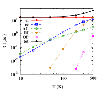
Figure 1: (Color online) Total SRT ($\blacktriangle$) and the contributions from the electron-impurity ($\bullet$), electron-electron Coulomb ($\square$), electron–AC-phonon ($\circ$), electron–RI-phonon ($\blacktriangledown$) as well as electron–OP-phonon ($\times$) scatterings as function of temperature $T$.

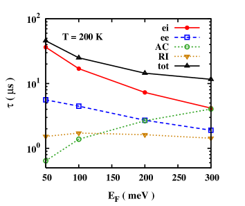
Figure 2: (Color online) Total SRT ($\blacktriangle$) and the contributions from the electron-impurity ($\bullet$), electron-electron Coulomb ($\square$), electron–AC-phonon ($\circ$) as well as electron–RI-phonon ($\blacktriangledown$) scatterings as function of Fermi energy $E_{\rm F}$. $T=200$ K.

Then we turn to the electron-density dependence. In Fig. 2, the total SRT and the contributions from various scatterings are plotted against the Fermi energy $E_{\rm F}$ at $T=200$ K.noRI It is seen that the SRT decreases first rapidly and then slowly with increasing $E_{\rm F}$. To understand the underlying physics, we first discuss the electron-density dependence of each individual scattering. The electron-impurity scattering decreases with $E_{\rm F}$ due to the decrease of the cross section.Guinea_08 The electron-electron Coulomb scattering also decreases with $E_{\rm F}$ in the degenerate regime due to the increase of the Pauli blocking.Jiang_bulk_09 The electron–AC-phonon scattering increases with increasing $E_{\rm F}$ since the matrix element ($\sim q$) and the density of states ($\sim k$) both increase with $E_{\rm F}$.Sarma_AC The electron–RI-phonon scattering varies slowly with $E_{\rm F}$ due to the competition of the decrease in the matrix element and the increase in the density of states.Fratini_RI Under the joint effects of these factors, the behaviour in $\tau-E_{\rm F}$ curve is understood: the SRT first decreases rapidly with $E_{\rm F}$ due to the decrease of the electron-impurity scattering, and then decreases slowly since the increase of the electron–AC-phonon scattering partially compensates the decrease of the impurity scattering.

The initial spin polarization dependence of the SRT is also investigated. In Fig. 3, we plot the SRT versus initial spin polarization $P$ at $T=20$ K and $200$ K. It is seen that the SRT increases rapidly with the increase of the initial spin polarization. By comparing the calculation with and without the Coulomb HF term, one can see that the increase of the SRT originates from the Coulomb HF term. The underlying physics is similar to the previous studies in semiconductors:highP the Coulomb HF term serves as an effective magnetic field along the $z$-axis, which is described by

$$B_{\rm HF}({\bf k})=\sum_{\mu{\bf k}^{\prime}}\left.V^{\mu 11}_{{\bf k},{\bf k}^{\prime}}I_{{\bf k}{\bf k}^{\prime}}(f_{\mu{\bf k}^{\prime}\frac{1}{2}}-f_{\mu{\bf k}^{\prime}-\frac{1}{2}})\right/(g\mu_{B}).$$ (10)

This effective magnetic field blocks the spin precession and slows down the spin relaxation. It is also shown that the SRT increases slower with $P$ when temperature increases. This is because at high temperature the electrons are distributed to a wider range in ${\bf k}$ space, thus the effective magnetic field becomes smaller [see Eq. (10)] and the effect of the HF term is weakened.highP It is noted that in graphene there is a considerable increase of the SRT with the initial spin polarization, even at room temperature. In contrast, in semiconductors the electron system is in the nondegenerate regime at room temperature (as the Fermi energy in semiconductor is only tens of meV), and thus the effect of the HF term becomes insignificant.highP This means that the HF effective field is more pronounced in graphene compared with semiconductors. Since the effects of the HF term have been probed experimentally in semiconductors recently,wu-exp-hP ; tobias ; Zheng_exp we expect they can be observed easily in graphene.

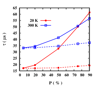
Figure 3: (Color online) SRT as function of initial spin polarization $P$ with (solid curves) and without (dashed curves) the Coulomb HF term at $T=20$ K ($\bullet$) and 300 K ($\square$).

We also study the effect of the in-plane electric field on spin relaxation. In Fig. 4, the SRT and the in-plane electric field $E_{\|}$ are plotted against the hot-electron temperature $T_{e}$ for lattice temperature $T=300$ K and applied magnetic field $B=2$ T. The hot-electron temperature is obtained by averaging the inverse of the slopes of $g_{\mu{\bf k}s}\equiv\log({1/f_{\mu{\bf k}s}^{\rm st}}-1)$ with ${\bf k}$ varying along different directions. Here $f_{\mu{\bf k}s}^{\rm st}$ represents the hot-electron distribution function in the steady state, whose expression will be discussed in the next subsection. From Fig. 4, it is seen that the SRT increases monotonically with the electric field, which is very different from the complicated behavior in semiconductor quantum wells.hot-e ; Zhou_PRB_07 In those systems, the high electric field induces two effects: (i) the drift of the electron distribution which enhances the inhomogeneous broadening as more electrons are distributed at larger $k$ and the SOC increases with $k$; (ii) the hot-electron effect which enhances the momentum scattering. The former tends to decrease the SRT while the latter tends to increase. Therefore the electric field dependence of the SRT can be nonmonotonic.hot-e ; Zhou_PRB_07 However, the spin-orbit field in graphene is independent on magnitude of ${\bf k}$. Thus Effect (i) on spin relaxation is marginal, and the electric field dependence of the SRT is mainly from the hot-electron effect. Consequently the SRT increases monotonically with $E_{\|}$. In addition, by comparing the calculation with and without the electron-electron Coulomb scattering at the same hot-electron temperature, one finds that the contribution to the SRT from the electron-electron scattering increases with increasing hot-electron temperature, which is consistent with the lattice temperature dependence discussed above.

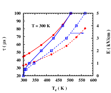
Figure 4: (Color online) SRTs ($\bullet$) and in-plane electric field $E_{\|}$ ($\square$) as function of hot-electron temperature $T_{e}$ with (solid curves) and without (dashed curves) the electron-electron Coulomb scattering at lattice temperature $T=300$ K and applied magnetic field in the Voigt configuration $B=2$ T.

III.2 Steady-state hot-electron distribution function

Previous investigations have shown that in the Boltzmann limit, the strong electron-electron Coulomb scattering can establish the steady-state hot-electron distribution functiondistribution

$$\tilde{f}^{\rm st}_{\mu{\bf k}s}=\left\{\exp\left[(\varepsilon_{{\mu}{\bf k}}-{\bf u}\cdot{\bf k}-\mu_{s})/(k_{B}T_{e})\right]+1\right\}^{-1},$$ (11)

where $\mu_{s}$ stands for the chemical potential of electrons with spin $s$ and ${\bf u}$ is the drift velocity. Recently Bistritzer and MacDonald applied this distribution function to study the charge transport in graphene.Bistritzer However, whether the Coulomb scattering in graphene is strong enough to justify the validity of this distribution function remains unchecked. Since we can obtain the distribution function with the genuine Coulomb scattering explicitly computed, we check the validity of Eq. (11) here. It is noted, if Eq. (11) is valid, $g_{\mu{\bf k}s}\equiv\log({1/\tilde{f}_{\mu{\bf k}s}^{\rm st}}-1)=(v_{\rm F}|{\bf k}|-{\bf u}\cdot{\bf k}-\mu_{s})/k_{B}T_{e}$ has a minimum around $k=0$ and different slopes along different $k$-directions. In Fig. 5(a), $g_{\mu{\bf k}s}$ is plotted against ${\bf k}$ varying along the direction of the electric field at $E_{\|}=2$ kV$/$cm and $T=300$ K. One immediately finds that the hot-electron distribution function from our calculation is very different from Eq. (11): the minimum of $g_{\mu{\bf k}s}$ is away from the point of $k=0$ and the slopes are close to each other when ${\bf k}$ varying along opposite directions. Based on the above property, we propose the approximate expression of the computed hot-electron distribution function as:

$$f^{\rm st}_{\mu{\bf k}s}=\left\{\exp\left[(\varepsilon_{{\mu}{\bf k}-{\bf u}}-\mu_{s})/k_{B}T_{e}\right]+1\right\}^{-1}.$$ (12)

Correspondingly, $g_{\mu{\bf k}s}=(v_{\rm F}|{\bf k}-{\bf u}|-\mu_{s})/k_{B}T_{e}$. To examine our assumption, we also plot $g_{\mu{\bf k}s}$ from Eq. (12) in Fig. 5(a) and find that the computed hot-electron distribution function is in reasonable agreement with Eq. (12). In fact, for systems with parabolic energy dispersion, e.g., semiconductors in our previous investigations,hot-e ; Jiang_bulk_09 Eqs. (11) and (12) are equivalent. However, for graphene with linear dispersion, these two distribution functions are quite distinct. It is noted that Eq. (12) is just used to estimate the hot-electron temperature. The SRT and hot-electron distribution in this investigation are explicitly computed from the KSBEs.

In order to reveal the effect of Coulomb scattering to the steady-state hot-electron distribution, we introduce a dimensionless scaling coefficient $\chi$ in front of the electron-electron Coulomb scattering, with $\chi=1$ corresponding to the genuine case. We plot $g_{\mu{\bf k}s}$ against ${\bf k}$ along the direction of the electric field with different scaling coefficients $\chi$ in Fig. 5(b). It is seen that with the increase of $\chi$, i.e., the electron-electron Coulomb scattering, the distribution function gets closer to Eq. (11). This indicates that in graphene the electron-electron Coulomb scattering is not strong enough to establish the hot-electron distribution Eq. (11).

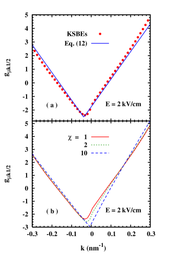
Figure 5: (Color online) (a) $g_{\mu{\bf k}\frac{1}{2}}\equiv\log({1/f^{\rm st}_{\mu{\bf k}\frac{1}{2}}}-1)$ from the KSBE computation (red dots) and from Eq. (12) (blue solid curve) against ${\bf k}$ varying along the direction of the in-plane electric field at $E_{\|}=2$ kV$/$cm and $T=300$ K. (b) $g_{\mu{\bf k}\frac{1}{2}}$ vs. ${\bf k}$ with the scaling coefficients $\chi=1$ (red solid curve), 2 (green dotted curve) and 10 (blue dashed curve).

IV Conclusion and Discussion

In conclusion, we have investigated the spin relaxation in graphene from the microscopic KBSE approach, where all the relevant scatterings, especially the electron-electron Coulomb scattering, are explicitly included. We show that the SRT remains almost unchanged with increasing $T$ at low temperature because the electron-impurity scattering, which dominates the momentum scattering, varies little with temperature. Nevertheless, the SRT increases with $T$ at high temperature because the electron-electron and electron-phonon scatterings become comparable to the electron-impurity scattering and both scatterings increase with increasing $T$. We also show that the electron-electron Coulomb scattering plays an important role in spin relaxation at high temperature. It is also seen that the SRT first decreases rapidly with the increase of $E_{\rm F}$ due to the decrease of the electron-impurity scattering, and then decreases mildly with $E_{\rm F}$ since the increase of the electron–AC-phonon scattering partially counteracts the decrease of the electron-impurity scattering. We also predict a pronounced increase of the SRT at high spin polarization in the whole temperature regime of our investigation. The underlying physics is that the Coulomb HF term serves as an effective longitudinal magnetic field which blocks the spin precession and suppresses the spin relaxation. The effect of the in-plane electric field on spin relaxation is also investigated. It is shown that the SRT increases with the in-plane electric field due to the hot-electron effect. Moreover, we show that the electron-electron Coulomb scattering in graphene is not strong enough to establish the usual steady-state hot-electron distribution in the literature and an approximate one is suggested based on our computation.

Now we address the effect of ripples on the spin relaxation. For graphene samples with an undulating surface, i.e. ripples,Morozov_curv an additional Rashba-type SOC, whose expression is the same as the electric field induced SOC,Hernando_06 appears. The SOC coefficient due to the curvature effect is estimated to be $\alpha_{\rm curv}{\sim}0.02$ meV (0.2 K),Hernando_06 which is about two orders of magnitude larger than $\alpha_{\rm R}=1.5\times 10^{-4}$ meV used in our calculations. For the well-known relation $1/\tau\propto\alpha_{\rm R}^{2}$ for the DP mechanism,Dyakonov one expects that the SRT is shortened by four orders of magnitude. Nevertheless, the additional SOC does not change the dependences of the SRT on the temperature and sample parameters, as well as the importance of the electron-electron Coulomb scattering.

Finally, it is noted that even after considering the SOC enhanced by the curvature effect, the SRTs from our calculation are still two orders of magnitude larger than those in recent spin transport experimental measurements.Tombros_07 ; Tombros_08 ; Popinciuc ; Jozsa_09 We stress that the range of impurity (adatom) density of the graphene samples we discuss is different from that in recent experiments, and therefore the dominant spin relaxation mechanism is also quite different. As mentioned above, the mechanism most likely limiting the SRTs in the recent experiments is the local spin-orbit field induced by the randomly distributed adatoms. The experimental and theoretical worksVarykhalov ; Castro_imp showed that the SOC strength from the adatoms can reach $10$ meV, which is about three orders of magnitude larger than the strength used in our calculations. The study on the effect of the adatoms on spin relaxation is beyond the scope of this investigation. It is further noted that the spin-related experiment in clean graphene is still missing, we expect that the effects presented in this manuscript can be confirmed by the future experiments in relatively cleaner graphene samples. A possible method to obtain the graphene sample with higher mobility is the epitaxial growth of graphene on SiC substrate.Emtsev ; Virojanadara ; Deretzis Nevertheless in this system, some other factors must be taken into account, e.g., the scattering arising from the interfacial states.Deretzis The study in this system can be the future extension of this investigation.

*

Appendix A Expression of the interaction Hamiltonian

The electron-impurity and electron-electron Coulomb interaction Hamiltonian can be written as

$$H_{ei} = \sum_{j{\mu}{\nu}\atop{\bf k}{\bf q}s}U^{\mu\nu}_{{\bf k},{\bf k}-{\bf q}}T^{{\mu}\nu\nu}_{{\bf k}{\bf k}-{\bf q}}e^{-i{\bf q}\cdot{\bf R}_{j}}{c^{{\mu}\nu}_{{\bf k}s}}^{\dagger}c^{{\mu}\nu}_{{\bf k}-{\bf q}s},$$ (13)

$$H_{ee} = \frac{1}{2}\sum_{{\mu}{\mu}^{\prime}\nu\nu^{\prime}\atop{\bf k}{\bf k}^{\prime}{\bf q}ss^{\prime}}V^{\mu\nu\nu}_{{\bf k},{\bf k}-{\bf q}}T^{{\mu}\nu\nu}_{{\bf k}{\bf k}-{\bf q}}T^{{\mu}^{\prime}\nu^{\prime}\nu^{\prime}}_{{\bf k}^{\prime}{\bf k}^{\prime}+q}{c^{{\mu}\nu}_{{\bf k}s}}^{\dagger}{c^{{\mu}^{\prime}\nu^{\prime}}_{{\bf k}^{\prime}s^{\prime}}}^{\dagger}c^{{\mu}^{\prime}\nu^{\prime}}_{{\bf k}^{\prime}+qs^{\prime}}c^{{\mu}\nu}_{{\bf k}-{\bf q}s}$$ (14)

$$\mbox{}\hskip 85.35826pt+\frac{1}{2}\sum_{{\mu}{\mu}^{\prime},\nu\neq\nu^{\prime}\atop{\bf k}{\bf k}^{\prime}{\bf q}ss^{\prime}}V^{\mu\nu\nu^{\prime}}_{{\bf k},{\bf k}-{\bf q}}T^{{\mu}\nu\nu^{\prime}}_{{\bf k}{\bf k}-{\bf q}}T^{{\mu}^{\prime}\nu^{\prime}\nu}_{{\bf k}^{\prime}{\bf k}^{\prime}+q}{c^{{\mu}\nu}_{{\bf k}s}}^{\dagger}{c^{{\mu}^{\prime}\nu^{\prime}}_{{\bf k}^{\prime}s^{\prime}}}^{\dagger}c^{{\mu}^{\prime}\nu}_{{\bf k}^{\prime}+qs^{\prime}}c^{{\mu}\nu^{\prime}}_{{\bf k}-{\bf q}s}.$$

In these equations, ${\bf R}_{j}$ stands for the position of $j$th impurity; $T^{{\mu}\nu\nu^{\prime}}_{{\bf k}{\bf k}-{\bf q}}={\psi_{{\bf k}}^{\mu\nu}}^{\dagger}\psi_{{\bf k}-{\bf q}}^{\mu\nu^{\prime}}$; $U^{\mu\nu}_{{\bf k},{\bf k}-{\bf q}}=Z_{i}V^{\mu\nu\nu}_{{\bf k},{\bf k}-{\bf q}}e^{-qd}$ is the electron-impurity interaction matrix element. Here $Z_{i}=1$ is the charge number of the impurity; the effective distance $d$ of the impurity layer to the graphene sheet is chosen to be $0.4$ nm.Fabian_SR ; Adam_07 ; Hwang_PRL ; Adam_08 ; Fratini_RI $V^{\mu\nu\nu^{\prime}}_{{\bf k},{\bf k}-{\bf q}}$ denotes the screened Coulomb potential where the screening is calculated under the random phase approximation,Manhan ; Jonson ; Zhou_PRB_07 ; Haug_1998 ; Adam_07 ; Hwang_PRL ; Adam_08 ; Sarma_Coulomb ; Sarma_RPA ; Wunsch ; Ramezanali ; WangXF

$$V^{\mu\nu\nu^{\prime}}_{{\bf k},{\bf k}-{\bf q}}=\frac{V_{{\bf q}}^{(0)}}{{1-V_{{\bf q}}^{(0)}\Pi({\bf q},\epsilon_{{\mu}\nu{\bf k}}-\epsilon_{{\mu}\nu^{\prime}{\bf k}-{\bf q}})}},$$ (15)

where $V_{{\bf q}}^{(0)}={{2\pi v_{\rm F}r_{s}}}/{q}$ is the two-dimensional bare Coulomb potential with $r_{s}=0.8$.Adam_07 ; Hwang_PRL ; Adam_08 As pointed out in Refs. Adam_07, and Hwang_PRL, , such small $r_{s}$ ensures the validity of the random phase approximation. $\Pi(\mathbf{q},\omega)$ is given byWunsch ; Sarma_RPA ; WangXF ; Ramezanali

$$\Pi(\mathbf{q},\omega)=\sum_{\mu\nu\nu^{\prime}{\bf k}s}|T^{{\mu}\nu\nu^{\prime}}_{{\bf k}{\bf k}-{\bf q}}|^{2}\frac{f^{\mu\nu}_{{\bf k}s}-f^{\mu\nu^{\prime}}_{{\bf k}-{\bf q}s}}{\epsilon_{\mu\nu{\bf k}}-\epsilon_{\mu\nu^{\prime}{\bf k}-{\bf q}}+\omega+i0^{+}}.$$ (16)

It is noted that the interband contribution in screening cannot be neglected even in the $n$-doped case.

The electron-phonon interaction Hamiltonian takes the form (only the terms relevant to the electron band presented)

$$H_{ep}=\sum_{{\mu}{\mu}^{\prime},\nu=1\atop{\bf k}{\bf q}s}M^{\lambda}_{\mu{\bf k},\mu^{\prime}{\bf k}-{\bf q}}(a_{{\lambda},{\bf q}}+a_{{\lambda},-{{\bf q}}}^{\dagger}){c^{{\mu}\nu}_{{\bf k}s}}^{\dagger}c^{{\mu}^{\prime}\nu}_{{\bf k}-{\bf q}s}.$$ (17)

Here $a_{{\lambda},{\bf q}}$ (${a_{{\lambda},{\bf q}}}^{\dagger}$) is the annihilation (creation) operator and $M^{\rm\lambda}_{\mu{\bf k},\mu^{\prime}{\bf k}-{\bf q}}$ stands for the matrix element of the electron-phonon interaction with $\lambda$ being the phonon branch index. For the electron–AC-phonon scattering, the phonon energy spectrum $\omega^{\rm AC}_{\bf q}=v_{\rm ph}q$ and $|M^{\rm AC}_{\mu{\bf k},\mu^{\prime}{\bf k}-{\bf q}}|^{2}=\frac{D^{2}q}{2\rho_{m}v_{\rm ph}}I_{{\bf k}{\bf k}-{\bf q}}\delta_{\mu\mu^{\prime}}$, where $v_{\rm ph}=2\times 10^{6}$ cm/s is acoustic phonon velocity and $\rho_{m}=7.6\times 10^{-8}$ g/cm² denotes graphene mass density.Sarma_AC ; Chen_Nnano The value of deformation potential $D$ is still in debate. The range of $D$ obtained via various theoretical and experimental methods is from $4.5$ to $30$ eV.Chen_Nnano ; Borysenko ; Bolotin ; Chen_AC ; Hong_AC ; Stauber ; Pietronero ; Sugihara Here we choose a moderate value $D=19$ eV.Sarma_AC ; Chen_Nnano ; Sugihara For the electron–RI-phonon scattering, $|M^{\rm RI}_{\mu{\bf k},\mu^{\prime}{\bf k}-{\bf q}}|^{2}=g\frac{v_{\rm F}^{2}}{a}\frac{e^{-2qd}}{q+q_{s}}I_{{\bf k}{\bf k}-{\bf q}}\delta_{\mu\mu^{\prime}}$ where $q_{s}=4r_{s}k_{\rm F}$ is the Thomas-Fermi screening length,Wunsch $a=1.42$ Å is the C-C bond distance. For SiO₂ substrate, the energy of the remote phonon modes are $\omega^{\rm RI}_{1}=59$ meV and $\omega^{\rm RI}_{2}=155$ meV; the corresponding dimensionless coupling parameters are $g_{1}=5.4\times 10^{-3}$ and $g_{2}=3.5\times 10^{-2}$, respectively.Fratini_RI The matrix element of the electron–OP-phonon scattering is described by $|M^{\rm OP}_{\mu{\bf k},\mu^{\prime}{\bf k}-{\bf q}}|^{2}=\frac{A_{\lambda}}{2\rho_{m}\omega_{\lambda}}$. For the longitudinal and transverse optical phonons near $\Gamma$ point, which cause the intravelley scattering, $A^{\rm LO}_{\Gamma}=\langle D_{\Gamma}^{2}\rangle[1-\cos(\theta_{\bf k}+\theta_{\bf k-q}-2\theta_{\bf q})]\delta_{\mu\mu^{\prime}}$, $A^{\rm TO}_{\Gamma}=\langle D_{\Gamma}^{2}\rangle[1+\cos(\theta_{\bf k}+\theta_{\bf k-q}-2\theta_{\bf q})]\delta_{\mu\mu^{\prime}}$ with $\langle D_{\Gamma}^{2}\rangle=45.60$ eV²/Ų and $\omega_{\Gamma}=196.0$ meV; whereas for the transverse optical phonon near $K(K^{\prime})$ point which causes the intervalley scattering, $A^{\rm TO}_{K}=\langle D_{K}^{2}\rangle[1-\cos(\theta_{\bf k}-\theta_{\bf k-q})]\delta_{\mu,-\mu^{\prime}}$ with $\langle D_{K}^{2}\rangle=92.05$ eV²/Ų and $\omega_{K}=161.2$ meV.Piscanec_OP ; Lazzeri_OP

References

- (1) A. K. Geim and K. S. Novoselov, Nature Mater. 6, 183 (2007).
- (2) J. Fischer, B. Trauzettel, and D. Loss, Phys. Rev. B 80, 155401 (2009).
- (3) C. L. Kane and E. J. Mele, Phys. Rev. Lett. 95, 226801 (2005).
- (4) D. Huertas-Hernando, F. Guinea, and A. Brataas, Phys. Rev. B 74, 155426 (2006).
- (5) H. Min, J. E. Hill, N. A. Sinitsyn, B. R. Sahu, L. Kleinman, and A. H. MacDonald, Phys. Rev. B 74, 165310 (2006).
- (6) Y. Yao, F. Ye, X.-L. Qi, S.-C. Zhang, and Z. Fang, Phys. Rev. B 75, 041401(R) (2007).
- (7) M. Gmitra, S. Konschuh, C. Ertler, C. Ambrosch-Draxl, and J. Fabian, Phys. Rev. B 80, 235431 (2009).
- (8) M. I. D’yakonov and V. I. Perel’, Zh. Eksp. Teor. Fiz. 60, 1954 (1971) [Sov. Phys. JETP 33, 1053 (1971)]; Fiz. Tverd. Tela (Leningrad) 13, 3581 (1971) [Sov. Phys. Solid State 13, 3023 (1972)].
- (9) D. Huertas-Hernando, F. Guinea, and A. Brataas, Eur. Phys. J. Spec. Top. 148, 177 (2007).
- (10) D. Huertas-Hernando, F. Guinea, and A. Brataas, Phys. Rev. Lett. 103, 146801 (2009).
- (11) C. Ertler, S. Konschuh, M. Gmitra, and J. Fabian, Phys. Rev. B 80, 041405(R) (2009).
- (12) M. W. Wu and C. Z. Ning, Eur. Phys. J. B 18, 373 (2000); M. W. Wu, J. Phys. Soc. Jpn. 70, 2195 (2001).
- (13) M. W. Wu, J. H. Jiang, and M. Q. Weng, Phys. Rep., doi:10.1016/j.physrep.2010.04.002 (2010) and references therein.
- (14) M. Q. Weng and M. W. Wu, Phys. Rev. B 68, 075312 (2003); ibid. 70, 195318 (2004).
- (15) D. Stich, J. Zhou, T. Korn, R. Schulz, D. Schuh, W. Wegscheider, M. W. Wu, and C. Schüller, Phys. Rev. Lett. 98, 176401 (2007); Phys. Rev. B 76, 205301 (2007).
- (16) T. Korn, D. Stich, R. Schulz, D. Schuh, W. Wegscheider, and C. Schüller, Adv. Solid State Phys. 48, 143 (2009).
- (17) F. Zhang, H. Z. Zheng, Y. Ji, J. Liu, and G. R. Li, Europhys. Lett. 83, 47006 (2008).
- (18) M. Q. Weng, M. W. Wu, and L. Jiang, Phys. Rev. B 69, 245320 (2004).
- (19) P. Zhang, J. Zhou, and M. W. Wu, Phys. Rev. B 77, 235323 (2008).
- (20) J. H. Jiang and M. W. Wu, Phys. Rev. B 79, 125206 (2009).
- (21) J. Zhou, J. L. Cheng, and M. W. Wu, Phys. Rev. B 75, 045305 (2007).
- (22) M. M. Glazov and E. L. Ivchenko, Pis’ma Zh. Eksp. Teor. Fiz. 75, 476 (2002) [JETP Lett. 75, 403 (2002)]; Zh. Eksp. Teor. Fiz. 126, 1465 (2004) [JETP 99, 1279 (2004)].
- (23) W. J. H. Leyland, G. H. John, R. T. Harley, M. M. Glazov, E. L. Ivchenko, D. A. Ritchie, I. Farrer, A. J. Shields, and M. Henini, Phys. Rev. B 75, 165309 (2007).
- (24) X. Z. Ruan, H. H. Luo, Y. Ji, Z. Y. Xu, and V. Umansky, Phys. Rev. B 77, 193307 (2008).
- (25) N. Tombros, C. Józsa, M. Popinciuc, H. T. Jonkman, and B. J. van Wees, Nature (London) 448, 571 (2007).
- (26) N. Tombros, S. Tanabe, A. Veligura, C. Józsa, M. Popinciuc, H. T. Jonkman, and B. J. van Wees, Phys. Rev. Lett. 101, 046601 (2008).
- (27) M. Popinciuc, C. Józsa, P. J. Zomer, N. Tombros, A. Veligura, H. T. Jonkman, and B. J. van Wees, Phys. Rev. B 80, 214427 (2009).
- (28) C. Józsa, T. Maassen, M. Popinciuc, P. J. Zomer, A. Veligura, H. T. Jonkman, and B. J. van Wees, Phys. Rev. B 80, 241403(R) (2009).
- (29) A. H. Castro Neto and F. Guinea, Phys. Rev. Lett. 103, 026804 (2009).
- (30) D. P. DiVincenzo and E. J. Mele, Phys. Rev. B 29, 1685 (1984).
- (31) Here we have corrected a minor error in Eq. (2) of Ref. Fabian_SR, .
- (32) K. S. Novoselov, A. K. Geim, S. V. Morozov, D. Jiang, Y. Zhang, S. V. Dubonos, I. V. Grigorieva, and A. A. Firsov, Science 306, 666 (2004).
- (33) As shown by Ertler et al.,Fabian_SR the charged impurities in the substrate also provide an random longitudinal electric field. However, for the impurity concentration cm-2 used in our calculation, the effective electric field from the charged impurities is smaller than kV/cm, and thus much smaller than the applied electric field used in the experiment.Novoselov_Science
- (34) H. Haug and A.-P. Jauho, Quantum kinetics in Transport and Optics of Semiconductors (Springer, Berlin, 1998).
- (35) The angle-resolved photoemission spectroscopy measurements [A. Bostwick, T. Ohta, T. Seyller, K. Horn, and E. Rotenberg, Nature Phys. 3, 36 (2007); K. R. Knox, S. Wang, A. Morgante, D. Cvetko, A. Locatelli, T. O. Mentes, M. A. Niño, P. Kim, and R. M. Osgood, Jr., Phys. Rev. B 78, 201408(R) (2008)] have shown that in the monolayer graphene grown on a weakly interacting substrate, the linear energy dispersion is a good approximation for the electrons in the energy range of our investigation, i.e., hundreds of meV above the bottom of the electron band.
- (36) C. Lü, J. L. Cheng, M. W. Wu, and I. C. da Cunha Lima, Phys. Lett. A 365, 501 (2007).
- (37) G. F. Giulianni and G. Vignale, Quantum Theory of the Electron Liquid (Cambridge University Press, Cambridge, England, 2005).
- (38) E. H. Hwang and S. Das Sarma, Phys. Rev. B 77, 115449 (2008).
- (39) J.-H. Chen, C. Jang, S. Xiao, M. Ishigami, and M. S. Fuhrer, Nat. Nanotechnol. 3, 206 (2008).
- (40) The contribution on spin relaxation from the electron–RI-phonon phonon is not shown here since it is much smaller than those from other scatterings at K.
- (41) F. Guinea, J. Low Temp. Phys. 153, 359 (2008).
- (42) S. Fratini and F. Guinea, Phys. Rev. B 77, 195415 (2008).
- (43) E. M. Lifshitz and L. P. Pitaevskii, Physical Kinetics (Pergamon, London, 1981); G. E. Uhlenbeck, G. W. Ford, and E. W. Montroll, Lectures in Statistical Mechanics (American Mathematical Society, Providence, 1963), Chap. IV; V. F. Gantmakher and Y. B. Levinson, Carrier Scattering in Metals and Semiconductors (North-Holland, Amsterdam, 1987), Chap. 6.
- (44) R. Bistritzer and A. H. MacDonald, Phys. Rev. B 80, 085109 (2009).
- (45) S. Morozov, K. Novoselov, M. Katsnelson, F. Schedin, D. Jiang, and A. K. Geim, Phys. Rev. Lett. 97, 016801 (2006).
- (46) A. Varykhalov, J. Sánchez-Barriga, A. M. Shikin, C. Biswas, E. Vescovo, A. Rybkin, D. Marchenko, and O. Rader, Phys. Rev. Lett. 101, 157601 (2008).
- (47) K. V. Emtsev, A. Bostwick, K. Horn, J. Jobst, G. L. Kellogg, L. Ley, J. L. McChesney, T. Ohta, S. A. Reshanov, J. Röhrl, E. Rotenberg, A. K. Schimd, D. Waldmann, H. B. Weber, and T. Seyller, Nature Mater. 8, 203 (2009).
- (48) C. Virojanadara, M. Syväjarvi, R. Yakimova, L. I. Johansson, A. A. Zakharov, and T. Balasubramanian, Phys. Rev. B 78, 245403 (2008).
- (49) I. Deretzis and A. La Magna, Appl. Phys. Lett. 95, 063111 (2009).
- (50) S. Adam, E. H. Hwang, V. M. Galitski, and S. Das Sarma, Proc. Natl. Acad. Sci. USA 104, 18392 (2007).
- (51) E. H. Hwang, S. Adam, and S. Das Sarma, Phys. Rev. Lett. 98, 186806 (2007).
- (52) S. Adam and S. Das Sarma, Solid State Commun. 146, 356 (2008).
- (53) G. D. Mahan, Many Particle Physics (Plenum, New York, 2000).
- (54) M. Jonson, J. Phys. C 9, 3055 (1976).
- (55) S. Das Sarma, E. H. Hwang, and W.-K. Tse, Phys. Rev. B 75, 121406(R) (2007); E. H. Hwang, B. Y.-K. Hu, and S. Das Sarma, ibid. 76, 115434 (2007).
- (56) E. H. Hwang and S. Das Sarma, Phys. Rev. B 75, 205418 (2007).
- (57) B. Wunsch, T. Stauber, F. Sols, and F. Guinea, New J. Phys. 8, 318 (2006).
- (58) X.-F. Wang and T. Chakraborty, Phys. Rev. B 75, 033408 (2007).
- (59) M. R. Ramezanali, M. M. Vazifeh, R. Asgari, M. Polini, and A. H. MacDonald, J. Phys. A: Math. Theor. 42, 214015 (2009).
- (60) S. Ono and K. Sugihara, J. Phys. Soc. Jpn. 21, 861 (1966); K. Sugihara, Phys. Rev. B 28, 2157 (1983).
- (61) K. I. Bolotin, K. J. Sikes, J. Hone, H. L. Stormer, and P. Kim, Phys. Rev. Lett. 101, 096802 (2008).
- (62) J.-H. Chen, C. Jang, M. Ishigami, S. Xiao, W. G. Cullen, E. D. Williams, and M. S. Fuhrer, Solid State Commun. 149, 1080 (2009).
- (63) X. Hong, A. Posadas, K. Zou, C. H. Ahn, and J. Zhu, Phys. Rev. Lett. 102, 136808 (2009).
- (64) K. M. Borysenko, J. T. Mullen, E. A. Barry, S. Paul, Y. G. Semenov, J. M. Zavada, M. B. Nardelli, and K. W. Kim, Phys. Rev. B 81, 121412(R) (2010).
- (65) T. Stauber, N. M. R. Peres, and F. Guinea, Phys. Rev. B 76, 205423 (2007); F. T. Vasko and V. Ryzhii, ibid. 76, 233404 (2007).
- (66) L. Pietronero, S. Strässler, H. R. Zeller, and M. J. Rice, Phys. Rev. B 22, 904 (1980); L. M. Woods and G. D. Mahan, ibid. 61, 10651 (2000); H. Suzuura and T. Ando, ibid. 65, 235412 (2002); G. Pennington and N. Goldsman, ibid. 68, 045426 (2003).
- (67) S. Piscanec, M. Lazzeri, F. Mauri, A. C. Ferrari, and J. Robertson, Phys. Rev. Lett. 93, 185503 (2004).
- (68) M. Lazzeri, S. Piscanec, F. Mauri, A. C. Ferrari, and J. Robertson, Phys. Rev. Lett. 95, 236802 (2005).