Magnetic phase diagram of the spin-$1/2$ antiferromagnetic zigzag ladder

Abstract

We study the one-dimensional spin-1/2 Heisenberg model with antiferromagnetic nearest-neighbor $J_{1}$ and next-nearest-neighbor $J_{2}$ exchange couplings in magnetic field $h$. With varying dimensionless parameters $J_{2}/J_{1}$ and $h/J_{1}$, the ground state of the model exhibits several phases including three gapped phases (dimer, $1/3$-magnetization plateau, and fully polarized phases) and four types of gapless Tomonaga-Luttinger liquid (TLL) phases which we dub TLL1, TLL2, spin-density-wave (SDW₂), and vector chiral phases. From extensive numerical calculations using the density-matrix renormalization-group method, we investigate various (multiple-)spin correlation functions in detail, and determine dominant and subleading correlations in each phase. For the one-component TLLs, i.e., the TLL1, SDW₂, and vector chiral phases, we fit the numerically obtained correlation functions to those calculated from effective low-energy theories of TLLs, and find good agreement between them. The low-energy theory for each critical TLL phase is thus identified, together with TLL parameters which control the exponents of power-law decaying correlation functions. For the TLL2 phase, we develop an effective low-energy theory of two-component TLL consisting of two free bosons (central charge $c=1+1$), which explains numerical results of entanglement entropy and Friedel oscillations of local magnetization. Implications of our results to possible magnetic phase transitions in real quasi-one-dimensional compounds are also discussed.

I Introduction

Frustrated quantum antiferromagnets have long been a subject of active research, since AndersonAnderson suggested resonating-valence-bond ground state for a triangular lattice antiferromagnet. Recent experimental studies of quasi-two-dimensional compounds, such as the organic Mott insulatorShimizu $\kappa$-(BEDT-TTF)₂Cu₂(CN)₃ and the transition metal chloride Cs₂CuCl₄,Coldea have further prompted theoretical research of anisotropic triangular lattice antiferromagnets.Watanabe04 ; Motrunich05 ; Lee2 ; Alicea06 ; Veillette05 ; StarykhB2007 ; Kawakami09 ; Kohno In these anisotropic quasi-two-dimensional antiferromagnets combination of frustrated exchange interactions and strong quantum fluctuations suppresses tendency toward conventional magnetic orders, thereby opening up possibilities of exotic quantum states.

A zigzag spin ladder is a one-dimensional (1D) strip of the anisotropic triangular lattice spin system, and can be regarded as a minimal, toy model of (strongly anisotropic quasi-two-dimensional) frustrated quantum magnets. Furthermore, the 1D $J_{1}$-$J_{2}$ Heisenberg model on the zigzag ladder is in itself a good model for various quasi-1D magnetic compounds, such as (N₂H₅)CuCl₃,Brown1979 ; Hagiwara2001 ; Maeshima2003 Rb₂Cu₂Mo₃O₁₂,Hase2004 and LiCuVO₄.Enderle2005 ; Banks2007 ; Buttgen2007 ; Naito2007 ; Schrettle2008 Despite its simplicity, the 1D $J_{1}$-$J_{2}$ Heisenberg model has been shown to exhibit various unconventional phases under magnetic field (as we summarize below).OkunishiT2003 ; HikiharaKMF2008 ; SudanLL2008 ; Heidrich-Meisner2009 In this paper we aim to clarify the nature of the phases in the ground-state phase diagram of the 1D spin-$1/2$ $J_{1}$-$J_{2}$ Heisenberg model under magnetic field, when both the nearest- and next-nearest-neighbor exchange couplings are antiferromagnetic (AF). To this end, we study in detail spin correlations in each phase using the numerical density matrix renormalization group (DMRG) method as well as low-energy effective theory based on bosonization.

The Hamiltonian of the $J_{1}$-$J_{2}$ Heisenberg zigzag spin ladder is given by

$$\mathcal{H}=J_{1}\sum_{l}{\bm{s}}_{l}\cdot{\bm{s}}_{l+1}+J_{2}\sum_{l}{\bm{s}}_{l}\cdot{\bm{s}}_{l+2}-h\sum_{l}s^{z}_{l},$$ (1)

where ${\bm{s}}_{l}$ is a spin-$1/2$ operator at $l$th site, $J_{1}$ and $J_{2}$ are respectively the nearest- and next-nearest-neighbor exchange couplings ($J_{1}>0$ and $J_{2}>0$), and $h$ is external magnetic field along the $z$-direction.

In the classical limit, the ground state of the zigzag ladder $J_{1}$-$J_{2}$ Heisenberg antiferromagnet has a helical magnetic structure

$${\bm{s}}_{l}=s(\sin\theta^{c}\cos\phi_{l}^{c},\sin\theta^{c}\sin\phi_{l}^{c},\cos\theta^{c})$$ (2)

with a pitch angle

$$\phi^{c}=\phi_{l+1}^{c}-\phi_{l}^{c}=\pm\arccos\left(\frac{-J_{1}}{4J_{2}}\right)$$ (3)

and a canting angle

$$\theta^{c}=\arccos\left(\frac{4hJ_{2}}{s(J_{1}+4J_{2})^{2}}\right)$$ (4)

for $J_{2}/J_{1}>1/4$, whereas the ground state has canted Néel order for $J_{2}/J_{1}\leq 1/4$.

In the quantum ($s=1/2$) case, the ground-state properties of the model (1) change drastically from the classical spin state. The ground state at zero magnetic field $h=0$ has been understood quite well. For small $J_{2}/J_{1}<(J_{2}/J_{1})_{\rm c}$, the ground state is in a critical Tomonaga-Luttinger liquid (TLL) phase with gapless excitations. The model undergoes a quantum phase transition at $(J_{2}/J_{1})_{\rm c}=0.2411$,JullienH1983 ; OkamotoN1992 ; Eggert1996 to a gapped phase with spontaneous dimerizationMajumdarG1969A ; MajumdarG1969B ; Haldane1982 ; WhiteA1996 for $J_{2}/J_{1}>(J_{2}/J_{1})_{\rm c}$. It is also known that the model exhibits a long-range order (LRO) of vector chirality in the case of anisotropic exchange couplings.NersesyanGE1998 ; KaburagiKH1999 ; HikiharaKK2001

With applied magnetic field, the phase diagram becomes even richer. From numerical studies of the magnetization process, it has been found that for a certain range of $J_{2}/J_{1}$ the magnetization curve exhibits a plateau at one-third of the saturated magnetization and cusp singularities.OkunishiT2003 ; OkunishiHA1999 ; OkunishiT2003B ; TonegawaOONK2004 In this $1/3$-plateau phase, the ground state has a magnetic LRO of up-up-down structure. Furthermore, it was found that away from the $1/3$-plateau and at $J_{2}/J_{1}\gtrsim 1$, the total magnetization $S^{z}_{\rm tot}=\sum_{l}s^{z}_{l}$ changes in units of $\Delta S^{z}_{\rm tot}=2$, indicating that two spins form a bound pair and flip simultaneously as the field $h$ increases.OkunishiT2003 ; OkunishiT2003B These characteristic changes in the magnetization process give accurate estimates of phase boundaries, which divide the parameter space into several regions (see Fig. 1 below), although the magnetization process alone cannot give much information on the nature of each phase.

Another interesting feature of the $J_{1}$-$J_{2}$ zigzag ladder in magnetic field is a field-induced LRO of the vector chirality,

$$\kappa_{l}^{(n)}=({\bm{s}}_{l}\times{\bm{s}}_{l+n})^{z}.$$ (5)

In zero field, the vector chiral LRO has been found when and only when the system has an easy-plane anisotropy.NersesyanGE1998 ; KaburagiKH1999 ; HikiharaKK2001 ; HikiharaKKT2000 ; Hikihara2002 In this case, due to the anisotropy, symmetry of the system in spin space is lowered from isotropic $SU(2)$ to $U(1)\times Z_{2}$, where the $U(1)$ and $Z_{2}$ symmetries correspond to the rotation in the easy plane and the sign of pitch angle of helical spin order, respectively. While the continuous $U(1)$ symmetry is preserved in the quantum case $s=|{\bm{s}}|<\infty$,Momoi1996 the discrete $Z_{2}$ symmetry can be spontaneously broken even in the quantum limit $s=1/2$, thereby resulting in the vector chiral phase. This line of symmetry consideration suggests that the magnetic field, which induces the same symmetry reduction, should also lead to the spontaneous symmetry breaking of the $Z_{2}$ symmetry. Indeed, this possibility was first pointed out by Kolezhuk and Vekua,KolezhukV2005 who have predicted from a field-theoretical analysis that the vector chiral LRO may set in for a large $J_{2}/J_{1}$ regime. Recently, the appearance of the vector chiral LRO under magnetic field was verified numerically.McCullochKKKSK2008 ; Okunishi2008

In this paper, we report our numerical and analytic results of the ground-state properties in the various phases that appear under magnetic field. From a thorough comparison of long-distance behavior of correlation functions, we identify effective theories that describe the low-energy physics of each phase. For this purpose, we calculate numerically various correlation functions, which include longitudinal-spin, transverse-spin, vector chiral, and nematic (two-magnon) correlation functions using the DMRG method.White1992 ; White1993 Comparing the numerical results with asymptotic forms derived from bosonization analysis, we find that, in addition to the gapped dimer phase, $1/3$-plateau phase, and fully polarized phase, the system exhibits four critical phases: (i) a phase with one-component TLL which is adiabatically connected to the ground state of the 1D Heisenberg antiferromagnet (TLL1 phase), (ii) a two-component TLL phase (TLL2 phase), (iii) a vector chiral phase, and (iv) a spin-density-wave phase with two-spin bound pairs (SDW₂ phase). The low-energy states in the TLL1, vector chiral, and SDW₂ phases turn out to be one-component TLLs (a conformal field theory with central charge $c=1$). Furthermore, we provide quantitative estimates of non-universal parameters appearing in the low-energy effective theories, such as the TLL parameter and incommensurate wavenumbers of spin correlations, as functions of $J_{2}/J_{1}$ and the magnetization. In particular, our results of the TLL parameter, which controls decay exponents of correlation functions, have direct relevance to experimental observables, e.g., a magnetic LRO emerging in real quasi-1D compounds with weak interladder couplings and temperature dependence of relaxation rates ($1/T_{1}$) in nuclear magnetic resonance experiments.Giamarchi-text ; SatoMF We also propose a two-component TLL theory to describe the TLL2 phase.

This paper is organized as follows: In Sec. II, we show the ground-state phase diagram under magnetic field (see Fig. 1), which contains the TLL1, $1/3$-plateau, SDW₂, vector chiral, TLL2, dimer, and fully polarized phases. We briefly summarize the characteristics of each phase. In the following sections, we discuss in detail our numerical results for correlation functions and effective theories for each phase. In Sec. III, we consider the TLL1 phase, which appears in small $J_{2}/J_{1}$ regime. The correlation functions obtained with the DMRG method are shown to be fitted well to analytic forms obtained from a bosonization theory for a weakly-perturbed single Heisenberg spin chain, and the decay exponents of the spin correlation functions are estimated accurately. This analysis reveals that the dominant correlation function changes from the staggered transverse-spin correlation to incommensurate longitudinal-spin one as $J_{2}/J_{1}$ increases. In Sec. IV, we discuss the SDW₂ phase, which appears at larger $J_{2}/J_{1}$. From the fitting of numerical data to bosonization theory, we show that the low-energy excitations are described by a one-component TLL with quasi-long-ranged dominant incommensurate longitudinal-spin and subleading nematic correlations and short-ranged transverse-spin correlation. Section V discusses the 1/3-plateau phase. We show that the numerically found up-up-down spin structure is understood in terms of the bosonization theories for the neighboring TLL1 and SDW₂ phases. In Sec. VI, we consider the vector chiral phase, which is also a one-component TLL. The fitting analysis shows that the vector chiral phase is characterized by the vector chiral LRO and the incommensurate quasi-LRO of the transverse spins. In Sec. VII, we develop a two-component TLL theory, i.e., two free boson theories (central charge $c=1+1$), as a low-energy effective theory for the TLL2 phase. We confirm the central charge $c=2$ through numerical computation of entanglement entropy. The consistency between the effective theory and the DMRG result is shown by examining a few dominant Fourier components in the local magnetization profile near open boundaries. Section VIII contains summary and discussions on implications of our results to real quasi-1D compounds with weak interladder couplings.

II Phase diagram

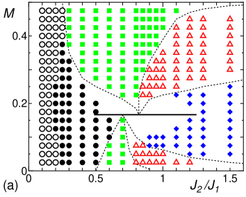
Figure 1: (Color online) Magnetic phase diagram of the spin-1/2 antiferromagnetic zigzag ladder (a) in the $J_{2}/J_{1}$ versus $M$ plane and (b) in the $J_{2}/J_{1}$ versus $h/J_{1}$ plane. In (a), symbols represent parameter points for which their ground-state phases are identified: Open ($\circ$) and solid ($\bullet$) circles represent the TLL1 phase with dominant transverse- and longitudinal-spin correlation, respectively. Diamonds ($\diamond$), triangles ($\vartriangle$), and squares ($\square$) respectively represent the SDW₂, vector chiral, and TLL2 phases. The solid line shows the 1/3-plateau phase. The dotted curves are the guide for the eye. In (b), symbols P, VC, D, and F indicate the 1/3 plateau, vector chiral, dimer, and fully polarized phases, respectively. The phase boundaries shown by solid lines are obtained in Ref. OkunishiT2003, from the numerical results of magnetization curves, except for the boundaries between the vector chiral and TLL2 phases which are obtained from the analysis of correlation functions in the present paper. The dotted line in the TLL1 phase represents the crossover line between the transverse- and longitudinal-spin dominant regimes.

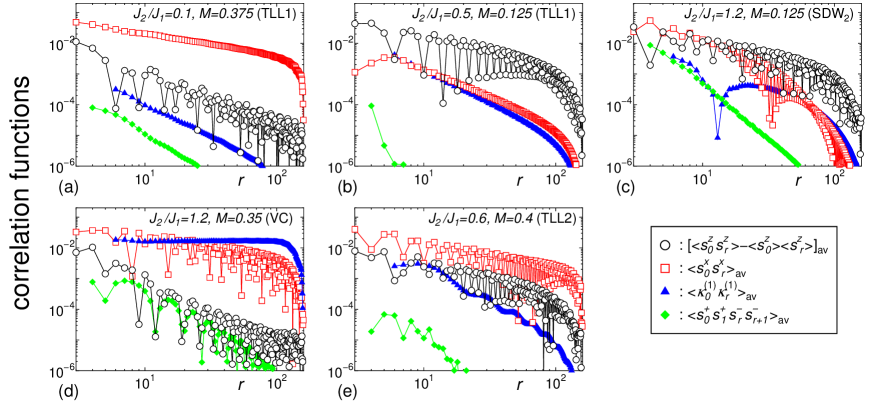
Figure 2: (Color online) Typical spatial dependence of correlation functions in critical phases; (a) TLL1 phase (transverse-spin correlation dominant), (b) TLL1 phase (longitudinal-spin correlation dominant), (c) SDW₂ phase, (d) vector chiral phase, and (e) TLL2 phase. Absolute values of the averaged correlation functions are plotted.

Figure 1 presents the magnetic phase diagram based on the numerical results obtained in this paper as well as in previous studies. The diagram is shown in the $J_{2}/J_{1}$ versus magnetization $M$ plane in Fig. 1(a) and in the $J_{2}/J_{1}$ versus $h/J_{1}$ plane in Fig. 1(b), where $M=(1/L)\sum_{l}s^{z}_{l}$ is the magnetization per site and $L$ the system size. The system exhibits at least four critical phases, i.e., TLL1, TLL2, vector chiral, and SDW₂ phases, in addition to three gapped phases including the dimer phase at $M=0$, the 1/3-plateau phase ($M=1/6$), and the fully polarized phase ($M=1/2$).

It has been revealed that the magnetization process of the zigzag ladder (1) has remarkable features:OkunishiT2003 ; OkunishiHA1999 ; OkunishiT2003B ; TonegawaOONK2004 for small $J_{2}/J_{1}$ ($0.25\leq J_{2}/J_{1}\lesssim 0.7$), the magnetization curve has at most two cusp singularities at higher and lower fields, $h=h_{\rm c1}$ and $h_{\rm c2}$, which correspond to boundaries between the TLL1 and TLL2 phases. A magnetization plateau also appears at $M=1/6$ for $0.487<J_{2}/J_{1}\lesssim 1.25$ and $h_{\rm p1}<h<h_{\rm p2}$.OkunishiT2003 ; TonegawaOONK2004 For large $J_{2}/J_{1}$, the magnetization process exhibits two-spin flips with $\Delta S^{z}_{\rm tot}=2$ in an intermediate field region $h_{\rm m1}<h<h_{\rm m2}$. See Figs. 2 and 3 in Ref. OkunishiT2003, for these results. At zero magnetization, the ground state is gapless for $J_{2}/J_{1}<0.2411$ and dimerized for $0.2411<J_{2}/J_{1}$. The spin gap in the dimerized phase vanishes at a critical field $h_{\mathrm{d}}$. The ground state is fully polarized above the saturation field $h_{\mathrm{s}}$. The critical fields $h_{\rm c1}$, $h_{\rm c2}$, $h_{\rm p1}$, $h_{\rm p2}$, $h_{\rm m1}$, $h_{\rm m2}$, $h_{\mathrm{d}}$, and $h_{\mathrm{s}}$ are plotted in Fig. 1(b) with solid lines.

To reveal the nature of ground states in each region, we have calculated several correlation functions, using the DMRG method, for the system with up to $L=160$ spins with open boundaries. We have kept typically $300$ block states in the calculation (up to $400$ states for some cases), and confirmed the convergence of the calculation by checking the dependence of results on the number of kept states. We have calculated the longitudinal-spin correlation function $\langle s^{z}_{l}s^{z}_{l^{\prime}}\rangle$, the transverse-spin correlation function $\langle s^{x}_{l}s^{x}_{l^{\prime}}\rangle$, the vector chiral correlation function $\langle\kappa_{l}^{(n)}\kappa_{l^{\prime}}^{(n^{\prime})}\rangle$ with $n,n^{\prime}=1,2$, the nematic (two-magnon) correlation function $\langle s^{+}_{l}s^{+}_{l+1}s^{-}_{l^{\prime}}s^{-}_{l^{\prime}+1}\rangle$, and the local spin polarization $\langle s^{z}_{l}\rangle$, where $\langle\cdots\rangle$ denotes the expectation value in the ground state. To lessen the open-boundary effects, we have computed the two-point correlation functions for several pairs of $(l,l^{\prime})$ with fixed distance $r=|l-l^{\prime}|$ and taken their average for the estimate of the correlation at the distance $r$. In the following, we use the notation $\langle\cdots\rangle_{\rm av}$ for the averaged correlation functions.

Figure 2 shows typical spatial dependence of averaged correlation functions in the critical phases. We note that the bending-down behaviors of the averaged correlation functions seen for large distance (e.g., $r\gtrsim 100$ for $L=160$) are due to boundary effects and should not be confused with intrinsic behaviors in the bulk. Analyzing the long-distance behavior of correlation functions in each parameter regime, we have determined the low-energy effective theory for each phase. The parameter points in the phase diagram at which numerical results are explained successfully by the effective low-energy theory of the corresponding phase are shown with symbols in Fig. 1(a). We summarize properties of each phase below.

TLL1 phase: In small $J_{2}/J_{1}$ regime, the ground state is adiabatically connected to the one-component TLL of the antiferromagnetic Heisenberg chain with only $J_{1}$ under magnetic field. For relatively large $J_{2}/J_{1}$ ($0.25\leq J_{2}/J_{1}$) the boundaries of the TLL1 phase are defined by the cusp singularities in the magnetization curve.OkunishiHA1999 ; OkunishiT2003 In this phase, both the longitudinal-spin fluctuation $\langle s^{z}_{0}s^{z}_{r}\rangle-\langle s^{z}_{0}\rangle\langle s^{z}_{r}\rangle$ and transverse-spin correlation functions $\langle s^{x}_{0}s^{x}_{r}\rangle$ decay algebraically. The former shows incommensurate oscillations with a wavenumber $Q=\pi(1\pm 2M)$, while the latter is staggered, $Q=\pi$. The numerical estimation of the decay exponents, shown in Sec. III, indicates that the dominant correlation function changes from the staggered transverse-spin correlation to incommensurate longitudinal-spin correlation as $J_{2}/J_{1}$ increases [see Figs. 2 (a) and (b)]. The TLL1 phase is thus divided by the crossover line into two regions of different dominant correlations, as shown in Fig. 1.

SDW₂ phase: For large $J_{2}/J_{1}$, there is a phase where the magnetization process changes by the steps of $\Delta S^{z}_{\rm tot}=2$.OkunishiT2003 We show in Sec. IV that this phase is described by a one-component TLL theory, which was originally derived from the weakly-coupled AF Heisenberg chains in the limit $J_{2}/J_{1}\gg 1$.KolezhukV2005 ; HMeisnerHV2006 ; VekuaHMH2007 ; HikiharaKMF2008 The phase is characterized by the quasi-long-ranged longitudinal-spin and nematic correlation functions, $\langle s^{z}_{0}s^{z}_{r}\rangle-\langle s^{z}_{0}\rangle\langle s^{z}_{r}\rangle$ and $\langle s^{+}_{0}s^{+}_{1}s^{-}_{r}s^{-}_{r+1}\rangle$, which are dual to each other, and by the short-ranged transverse-spin correlation function $\langle s^{x}_{0}s^{x}_{r}\rangle$ reflecting a finite energy gap to single-spin-flip excitations, as shown in Fig. 2(c). The longitudinal-spin correlation is incommensurate with the wavenumber $Q_{2}=\pm\pi(1/2+M)$. Numerical analyses of correlation functions reveal that the longitudinal-spin correlation function is dominant in the whole parameter region of this phase. We thus call this phase the SDW₂ phase. We note that the same phase has been found in the zigzag ladder (1) with ferromagnetic $J_{1}$ and AF $J_{2}$ as well.Chubukov1991 ; CabraHP2000 ; HMeisnerHV2006 ; KeckeMF2007 ; VekuaHMH2007 ; HikiharaKMF2008 ; SudanLL2008 ; LauchliSL2009

1/3-plateau phase: At one third of the saturated magnetization, $M=1/6$, there is a magnetization-plateau phase in the intermediate parameter region $0.487\lesssim J_{2}/J_{1}\lesssim 1.25$.OkunishiT2003 ; TonegawaOONK2004 This phase is characterized by a field-induced excitation gap and a spontaneous breaking of translational symmetry accompanied by a magnetic LRO of the up-up-down structure. The ground state is three-fold degenerate. As shown in Sec. V, all two-point correlation functions exhibit exponential decay, in accordance with the fully-gapped nature of the phase.

Vector Chiral phase: The vector chiral phase is characterized by the LRO of the vector chirality $\kappa^{(n)}$ as well as quasi-LRO of incommensurate transverse spins, which decays algebraically in space. The discrete $Z_{2}$ symmetry corresponding to the parity about a bond center is broken spontaneously and the ground state is doubly degenerate in the thermodynamic limit. This vector chiral state is a quantum counterpart of the classical helical state. Though the classical helical state appears in $1/4<J_{2}/J_{1}$ for arbitrary magnetization, the quantum vector chiral phase is found only in two narrow regions separated by the SDW₂ and 1/3-plateau phases,McCullochKKKSK2008 ; Okunishi2008 see Fig. 1. We show that the vector chiral phase is also described by a one-component TLL theory which can be formulated starting from the two weakly-coupled AF Heisenberg chains for $J_{2}/J_{1}\gg 1$.NersesyanGE1998 ; KolezhukV2005 The correlation functions in this phase will be discussed in Sec. VI.

TLL2 phase: The TLL2 phase occupies two parameter regions adjacent to the TLL1 phase and the vector chiral phase. The TLL2 phase is described as two Gaussian conformal field theories (central charge $c=1+1$), or a two-component TLL, having two flavors of free massless bosonic fields as its low-energy excitations. In the Jordan-Wigner fermion representation, fermions have two separate Fermi seas, and the two bosonic fields represent particle-hole excitations near the two sets of Fermi points. In the TLL2 phase all correlation functions decay algebraically and have incommensurate wave numbers which are linear functions of the two Fermi momenta of Jordan-Wigner fermions. We will discuss these properties and the low-energy effective theory in Sec. VII.

Dimer phase: For $J_{2}/J_{1}>0.2411$ and at $M=0$, the ground state of the $J_{1}$-$J_{2}$ AF Heisenberg zigzag spin ladder is spontaneously dimerized.MajumdarG1969A ; MajumdarG1969B ; Haldane1982 ; WhiteA1996 ; JullienH1983 ; OkamotoN1992 ; Eggert1996 The ground state is doubly degenerate in the thermodynamic limit, and there is a gap to lowest excitation.

Fully polarized phase: When applied magnetic field is larger than the saturation field, $h>h_{\rm s}$, the ground state is in the fully polarized phase with saturated magnetization $M=1/2$. As the field decreases, the fully-polarized ground state is destabilized by softening of single-magnon excitations, which have the dispersion,

$$\varepsilon_{k}=J_{1}(\cos k-1)+J_{2}(\cos 2k-1)+h.$$ (6)

When $J_{2}/J_{1}<1/4$, the magnon dispersion has a single minimum at $k=\pi$, while, when $J_{2}/J_{1}>1/4$, there are two energy minima at $k=\pm\arccos(-J_{1}/4J_{2})$. The saturation field $h_{\rm s}$ is given by $h_{\rm s}/J_{1}=2$ for $J_{2}/J_{1}<1/4$ and $h_{\rm s}/J_{1}=2J_{2}/J_{1}+1+J_{1}/(8J_{2})$ for $J_{2}/J_{1}>1/4$.

III TLL1 phase

In this section, we discuss the TLL1 phase appearing for small $J_{2}/J_{1}$. Since the parameter space of this phase includes the AF Heisenberg chain with $J_{2}=0$, we naturally expect that the TLL1 phase should share the same properties with the single Heisenberg chain. Here, we first briefly review the TLL theory for the AF Heisenberg zigzag ladder with weak $J_{2}$ coupling. We then compare the theory with the numerical results of correlation functions for the zigzag ladder (1) with $J_{2}>0$.

It is well known that the low-energy properties of a single Heisenberg chain under magnetic field ($|M|<\frac{1}{2}$ and $J_{2}=0$) is described as a TLL.Giamarchi-text Since the (leading) operator generated from weak $J_{2}$ coupling is irrelevant in applied magnetic field (and marginally irrelevant without magnetic field) in the renormalization-group sense, the low-energy effective theory for small $J_{2}/J_{1}$ is adiabatically connected to the TLL theory of the single AF Heisenberg chain ($J_{2}=0$). Hence the low-energy excitations in the TLL1 phase are free massless bosons governed by the Gaussian model,

$$\widetilde{\mathcal{H}}_{0}=\frac{v}{2}\int dx\left[K\left(\frac{d\theta}{dx}\right)^{2}+\frac{1}{K}\left(\frac{d\phi}{dx}\right)^{2}\right],$$ (7)

where $(\phi,\theta)$ are bosonic fields satisfying the equal-time commutation relation $[\phi(x),\partial_{y}\theta(y)]=i\delta(x-y)$. The TLL parameter $K$ is a function of $J_{2}/J_{1}$ and $M$. We have taken the lattice spacing to be one and identify the continuous coordinate $x$ with the site index $l$. The spin velocity $v$ is of order $J_{1}$, except for the saturation limit $M\to 1/2$, where $v\to 0$. The spin operators ${\bm{s}}_{l}$ can be expressed in terms of the bosonic fields as

$$s^{z}_{l}\!\! = \!\!M+\frac{1}{\sqrt{\pi}}\frac{d\phi(x)}{dx}$$ (8)

$$\!\!{}-(-1)^{l}a\sin[2\pi Ml+\sqrt{4\pi}\phi(x)]+\cdots,$$

$$s^{+}_{l}\!\! = \!\!(-1)^{l}be^{i\sqrt{\pi}\theta(x)}$$ (9)

$$\!\!{}+b^{\prime}e^{i\sqrt{\pi}\theta(x)}\sin[2\pi Ml+\sqrt{4\pi}\phi(x)]+\cdots,$$

where $a$, $b$, and $b^{\prime}$ are nonuniversal positive constants, whose numerical values are known at $J_{2}=0$.HikiharaF1998 ; HikiharaF2001 ; HikiharaF2004 Equations (7), (8), and (9) define the effective theory for the TLL1 phase, with which asymptotic forms of spin correlation functions are obtained as

$$\langle s^{z}_{0}s^{z}_{r}\rangle\!\! = \!\!M^{2}-\frac{\eta}{4\pi^{2}r^{2}}+A^{z}_{1}\frac{(-1)^{r}\cos(2\pi Mr)}{|r|^{\eta}}+\cdots,\quad$$ (10)

$$\langle s^{x}_{0}s^{x}_{r}\rangle\!\! = \!\!A^{x}_{0}\frac{(-1)^{r}}{|r|^{1/\eta}}-A^{x}_{1}\frac{\cos(2\pi Mr)}{|r|^{\eta+1/\eta}}+\cdots,$$ (11)

where $A^{z}_{1}=a^{2}/2$, $A^{x}_{0}=b^{2}/2$, $A^{x}_{1}=b^{\prime 2}/4$ (with appropriate short-distance regularization), and the decay exponent $\eta$ is related to the TLL parameter $K$ by $\eta=2K$. Equations (10) and (11) tell us that for $\eta>1$ the staggered transverse-spin correlation function $\langle s^{x}_{l}s^{x}_{l^{\prime}}\rangle$ is dominant, while the incommensurate longitudinal-spin correlation $\langle s^{z}_{l}s^{z}_{l^{\prime}}\rangle$ with a wavenumber $Q=\pi(1\pm 2M)$ is dominant for $\eta<1$. At $J_{2}=0$ the decay exponent $\eta$ can be calculated exactly using Bethe ansatz;BogoliubovIK1986 ; CabraHP1998 $\eta$ increases monotonically as $M$ increases, from $\eta=1$ at $M=0$ to $\eta=2$ for $M\to 1/2$. Therefore, at $J_{2}=0$, the transverse-spin correlation $\langle s^{x}_{0}s^{x}_{r}\rangle$ is always the most-slowly decaying one for $0<M<1/2$. For finite $J_{2}>0$, the exact value of the exponent $\eta$ is known in the limit $M\to 0$. For $J_{2}/J_{1}<0.2411$ where the ground state at $M=0$ is in the TLL1 phase, $\eta=1$ at $M=0$ because of the SU(2) symmetry. On the other hand, for $J_{2}/J_{1}>0.2411$, i.e., when the ground state at $M=0$ is in the dimer phase,Schulz1980 ; ChitraG1997 $\eta\to 1/2$ as $M\to 0$. This means that $\eta$ is singular at $J_{2}/J_{1}=(J_{2}/J_{1})_{c}$ and $M=0$.

One can also derive the (same) effective theory for the TLL1 phase, starting from the saturation limit for $0<J_{2}/J_{1}<1/4$. In this limit the system can be viewed as a dilute gas of interacting hard-core bosons (magnons) with one flavor, as the magnon dispersion (6) has a single minimum at $k=\pi$. The hydrodynamic theory for the one-flavor interacting bosons is nothing but the TLL theory, Eq. (7).Giamarchi-text This approach naturally gives the same asymptotic forms of spin correlators as Eqs. (8) and (9). Furthermore, in the saturation limit $M\to 1/2$, $\eta\to 2$ in the TLL1 phase (i.e., $J_{2}/J_{1}<1/4$), since the dilute limit of the hard-core bose gas is equivalent to a free fermion gas.

Next we discuss our DMRG results of the transverse and longitudinal spin correlation functions $\langle s^{x}_{l}s^{x}_{l^{\prime}}\rangle$ and $\langle s^{z}_{l}s^{z}_{l^{\prime}}\rangle$ and the local spin polarization $\langle s^{z}_{l}\rangle$. To achieve better numerical convergence and efficiency, the DMRG calculation was done for finite systems ($L$ spins) with open boundaries. We thus compare the numerical results with the correlation functions calculated analytically from the effective theory (7) by imposing appropriate boundary conditions on the bosonic field $\phi$.HikiharaF1998 ; HikiharaF2001 ; HikiharaF2004 To this end, we have taken the Dirichlet boundary conditions $\phi(\delta)=\phi(L+1-\delta)=0$,Fath2003 where $\delta$ is a free parameter to be determined later. For example, spatial dependence of the magnetization is given by

$$\langle s^{z}_{l}\rangle=z(l;q)\equiv\frac{q}{2\pi}-a\frac{(-1)^{l}\sin[q(l-\delta)]}{f_{\eta/2}\biglb(2(l-\delta)\bigrb)},$$ (12)

where

$$q=\frac{2\pi LM}{L+1-2\delta},$$ (13)

and

$$f_{\alpha}(x)=\left[\frac{2(L+1-2\delta)}{\pi}\sin\left(\frac{\pi|x|}{2(L+1-2\delta)}\right)\right]^{\alpha}.$$ (14)

In the limit $l\ll L$, Eq. (12) reduces to

$$\langle s^{z}_{l}\rangle=M-\frac{(-1)^{l}a}{[2(l-\delta)]^{\eta/2}}\sin[2\pi M(l-\delta)].$$ (15)

The presence of open boundaries gives rise to “Friedel oscillations” in the local magnetization. The wave number of the oscillations is “$2k_{F}$” of the Jordan-Wigner fermions, which equals $Q=\pi(1\pm 2M)$ for $L\gg 1$. Similarly, the longitudinal and transverse spin correlation functions are modified by boundary contributions as

$$\langle s^{z}_{l}s^{z}_{l^{\prime}}\rangle\!\! = \!\!Z(l,l^{\prime};q)$$ (16)

$$\equiv \!\!\left(\frac{q}{2\pi}\right)^{2}-\frac{\eta}{4\pi^{2}}\left[\frac{1}{f_{2}(l-l^{\prime})}+\frac{1}{f_{2}(l+l^{\prime}-2\delta)}\right]-\frac{qa}{2\pi}\left[\frac{(-1)^{l}\sin[q(l-\delta)]}{f_{\eta/2}\biglb(2(l-\delta)\bigrb)}+\frac{(-1)^{l^{\prime}}\sin[q(l^{\prime}-\delta)]}{f_{\eta/2}\biglb(2(l^{\prime}-\delta)\bigrb)}\right]$$

$$\!\!{}+\frac{(-1)^{l-l^{\prime}}a^{2}}{2f_{\eta/2}\biglb(2(l-\delta)\bigrb)f_{\eta/2}\biglb(2(l^{\prime}-\delta)\bigrb)}\left\{\cos[q(l-l^{\prime})]\frac{f_{\eta}(l+l^{\prime}-2\delta)}{f_{\eta}(l-l^{\prime})}-\cos[q(l+l^{\prime}-2\delta)]\frac{f_{\eta}(l-l^{\prime})}{f_{\eta}(l+l^{\prime}-2\delta)}\right\}$$

$$-\frac{\eta a}{2\pi}\!\left\{\frac{(-1)^{l}\cos[q(l-\delta)]}{f_{\eta/2}\biglb(2(l-\delta)\bigrb)}[g(l+l^{\prime}-2\delta)+g(l-l^{\prime})]+\frac{(-1)^{l^{\prime}}\cos[q(l^{\prime}-\delta)]}{f_{\eta/2}\biglb(2(l^{\prime}-\delta)\bigrb)}[g(l+l^{\prime}-2\delta)-g(l-l^{\prime})]\right\},$$

$$\langle s^{z}_{l}s^{z}_{l^{\prime}}\rangle\!\! - \!\!\langle s^{z}_{l}\rangle\langle s^{z}_{l^{\prime}}\rangle=Z(l,l^{\prime};q)-z(l;q)z(l^{\prime};q),$$ (17)

$$\langle s^{x}_{l}s^{x}_{l^{\prime}}\rangle\!\! = \!\!X(l,l^{\prime};q)$$ (18)

$$\equiv \!\!\frac{f_{1/2\eta}\biglb(2(l-\delta)\bigrb)f_{1/2\eta}\biglb(2(l^{\prime}-\delta)\bigrb)}{f_{1/\eta}(l-l^{\prime})f_{1/\eta}(l+l^{\prime}-2\delta)}\left\{\frac{(-1)^{l-l^{\prime}}b^{2}}{2}+\frac{{\rm sgn}(l-l^{\prime})bb^{\prime}}{2}\left[\frac{(-1)^{l^{\prime}}\cos[q(l-\delta)]}{f_{\eta/2}\biglb(2(l-\delta)\bigrb)}-\frac{(-1)^{l}\cos[q(l^{\prime}-\delta)]}{f_{\eta/2}\biglb(2(l^{\prime}-\delta)\bigrb)}\right]\right.$$

$$\!\!\left.-\frac{b^{\prime 2}}{4f_{\eta/2}\biglb(2(l-\delta)\bigrb)f_{\eta/2}\biglb(2(l^{\prime}-\delta)\bigrb)}\left[\cos[q(l+l^{\prime}-2\delta)]\frac{f_{\eta}(l-l^{\prime})}{f_{\eta}(l+l^{\prime}-2\delta)}+\cos[q(l-l^{\prime})]\frac{f_{\eta}(l+l^{\prime}-2\delta)}{f_{\eta}(l-l^{\prime})}\right]\right\},$$

where

$$g(x)=\frac{\pi}{2(L+1-2\delta)}\cot\!\left[\frac{\pi x}{2(L+1-2\delta)}\right].$$ (19)

In the limit $|L/2-l|\ll L$ and $|L/2-l^{\prime}|\ll L$, boundary effects go away, and Eqs. (16) and (18) reduce to Eqs. (10) and (11). In the fitting procedure discussed below, we have optimized $\delta$ to achieve the best fitting of $\langle s^{z}_{l}\rangle$ and $\langle s^{z}_{l}s^{z}_{l^{\prime}}\rangle-\langle s^{z}_{l}\rangle\langle s^{z}_{l^{\prime}}\rangle$, whereas we set $\delta=0$ for $\langle s^{x}_{l}s^{x}_{l^{\prime}}\rangle$ as it has turned out that the numerical data of $\langle s^{x}_{l}s^{x}_{l^{\prime}}\rangle$ can be fitted sufficiently well without optimizing $\delta$.

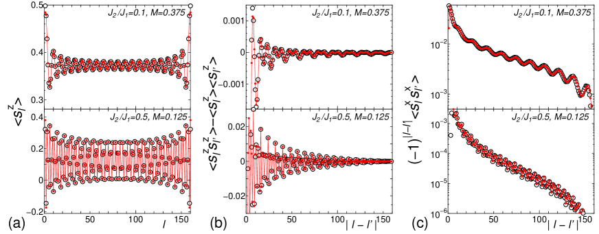
Figure 3: (Color online) Correlation functions in the antiferromagnetic zigzag ladder with $L=160$ spins in the TLL1 phase; (a) local spin polarization $\langle s^{z}_{l}\rangle$, (b) longitudinal-spin fluctuation $\langle s^{z}_{l}s^{z}_{l^{\prime}}\rangle-\langle s^{z}_{l}\rangle\langle s^{z}_{l^{\prime}}\rangle$, and (c) transverse-spin correlation function $\langle s^{x}_{l}s^{x}_{l^{\prime}}\rangle$. The upper and lower panels show the results for $(J_{2}/J_{1},M)=(0.1,0.375)$ and $(0.5,0.125)$, respectively. The open symbols represent the DMRG data and the solid lines and circles are fits to Eqs. (12), (17), and (18). In (b) and (c), the data for $l=L/2-[r/2]$ and $l^{\prime}=L/2+[(r+1)/2]$ are shown as a function of $r=|l-l^{\prime}|$.

Figure 3 shows DMRG data of $\langle s^{z}_{l}\rangle$, $\langle s^{z}_{l}s^{z}_{l^{\prime}}\rangle-\langle s^{z}_{l}\rangle\langle s^{z}_{l^{\prime}}\rangle$, and $\langle s^{x}_{l}s^{x}_{l^{\prime}}\rangle$ for $(J_{2}/J_{1},M)=(0.1,0.375)$ and $(0.5,0.125)$. In the same figures, we show the fits to Eqs. (12), (17), and (18). Clearly, the fits are in excellent agreement with the numerical results. We emphasize that only three fitting parameters, $\eta$, $\delta$, and $a$ ($\eta$, $b$, and $b^{\prime}$) are used in the fitting of $\langle s^{z}_{l}\rangle$ and $\langle s^{z}_{l}s^{z}_{l^{\prime}}\rangle-\langle s^{z}_{l}\rangle\langle s^{z}_{l^{\prime}}\rangle$ ($\langle s^{x}_{l}s^{x}_{l^{\prime}}\rangle$). We have obtained almost the same good quality of fits for the parameter points marked by open and solid circles in Fig. 1(b), which cover almost the entire region of the TLL1 phase. These results thus demonstrate that the TLL1 phase is described by the effective TLL theory given by Eqs. (7), (8), and (9), which is indeed the same TLL theory as that of the AF Heisenberg chain ($J_{2}=0$).

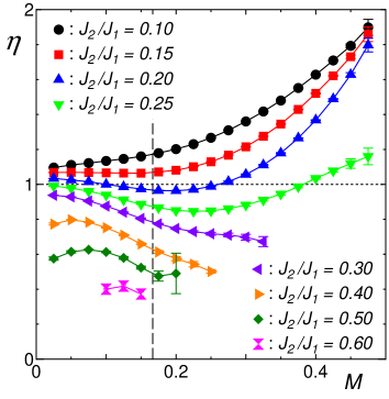
Figure 4: (Color online) $M$ dependence of the exponent $\eta$ for the TLL1 phase estimated from the fitting of $\langle s^{x}_{l}s^{x}_{l^{\prime}}\rangle$ for the antiferromagnetic zigzag ladder with $L=160$ spins. The error bars represent the difference of the estimates obtained from the fitting of the data of different ranges. The vertical dashed line corresponds to $M=1/6$ where the 1/3-plateau can appear for large $J_{2}/J_{1}$. The dotted line at $\eta=1$ represents the boundary between the regimes of dominant staggered transverse-spin correlation ($\eta>1$) and dominant incommensurate longitudinal-spin correlation ($\eta<1$); see Eqs. (10) and (11). The exponent $\eta$ relates to the parameter $K$ as $\eta=2K$ in the TLL theory for the TLL1 phase.

Figure 4 shows dependence of the exponent $\eta$ on the magnetization $M$ in the TLL1 phase, obtained from the fitting of the transverse-spin correlation $\langle s^{x}_{l}s^{x}_{l^{\prime}}\rangle$. Similar estimates of $\eta$ are obtained from the other correlators (not shown). For small $J_{2}/J_{1}$, $\eta$ exhibits essentially the same behavior as a function of $M$ as $\eta(M)$ at $J_{2}=0$; for $J_{2}/J_{1}\lesssim 0.15$, $\eta$ increases monotonically from the universal value $\eta=1$ at $M=0$ to $\eta=2$ at $M\to 1/2$ as $M$ increases. In this regime the transverse-spin correlation $\langle s^{x}_{0}s^{x}_{l}\rangle$ is dominant for any $M$. The situation changes as $J_{2}/J_{1}$ gets larger. With increasing $J_{2}/J_{1}$, $\eta$ decreases and becomes smaller than 1 at $J_{2}/J_{1}=0.2$ for intermediate magnetization $M$. As $J_{2}/J_{1}$ is further increased in the TLL1 phase, the exponent $\eta$ gets smaller than 1 for any $M$. Thus, the system undergoes a crossover from the small $J_{2}/J_{1}$ region with the dominant staggered transverse-spin correlation to the large $J_{2}/J_{1}$ region where the incommensurate longitudinal-spin correlation with $Q=\pi(1\pm 2M)$ is dominant. The crossover line is shown in the phase diagram, Fig. 1. The result is consistent with the earlier study,Gerhardt1997 in which $\eta$ was estimated at $M=1/6,1/4$ and $1/3$ for small systems. Such a crossover between ground states with the different dominant spin correlations has also been found for the $J_{1}$-$J_{2}$ zigzag ladder with bond alternation.UsamiS1998 ; HagaS2000 ; SuzukiS2004 ; MaeshimaOOS2004

As mentioned above, $\eta$ is expected to approach $1/2$ as $M\to 0$ for $J_{2}/J_{1}>(J_{2}/J_{1})_{\rm c}=0.2411$. Our numerical results at $J_{2}/J_{1}=0.5$ are consistent with this theoretical prediction. However, as $J_{2}/J_{1}$ approaches $(J_{2}/J_{1})_{\rm c}$ from above, the value of $\eta$ at the smallest $M=0.025$ becomes larger toward $\eta=1$, the value expected for $J_{2}/J_{1}<(J_{2}/J_{1})_{\mathrm{c}}$. This implies that $\eta$ increases very rapidly from 1/2 at small $M$ for this parameter regime of $J_{2}/J_{1}\lesssim 0.3$, where the spin gap in the dimer ground state at $M=0$ is exponentially small (thereby small $M$ is sufficient to wipe out dimer instability).

The data points for $0.3\leq J_{2}/J_{1}\leq 0.5$ end at the boundary to the TLL2 phase for larger $M$. Our results seem to indicate that $\eta$ changes continuously along the TLL1-TLL2 phase boundary.

When the magnetization is close to $M=1/6$, the TLL1 phase has an instability to the 1/3-plateau phase. In the Jordan-Wigner fermion picture, the instability is caused by umklapp scattering of three fermions, and the 1/3-plateau phase corresponds to a density wave state of the fermions.LecheminantO2004 ; HidaA2005 The three-particle umklapp scattering is irrelevant at small $J_{2}/J_{1}$ but becomes relevant for larger $J_{2}/J_{1}$. This explains why the 1/3-plateau phase emerges at $J_{2}/J_{1}\gtrsim 0.5$ in the phase diagram (Fig. 1), as we discuss below.

The effective Hamiltonian yielding the 1/3-plateau has the formLecheminantO2004 ; HidaA2005 ; Notephi

$$\widetilde{\mathcal{H}}=\widetilde{\mathcal{H}}_{0}+\lambda\int dx\sin\!\left[\pi(6M-1)x+3\sqrt{4\pi}\phi(x)\right],$$ (20)

where $\widetilde{\mathcal{H}}_{0}$ is the Gaussian model (7) for the TLL1 phase and $\lambda$ is the coupling constant for the three-particle umklapp scattering. The umklapp term is accompanied by an oscillating factor with a wavenumber $\pi(6M-1)\equiv 3\pi(1+2M)$ and becomes uniform at $M=1/6$. If we fix the magnetization at $M=1/6$ and increase $J_{2}/J_{1}$, then the three-particle umklapp term becomes relevant for $K<2/9$ ($\eta<4/9$). Indeed, we see in Fig. 4 that the estimates of $\eta$ near $M=1/6$ are larger than $4/9$ for $J_{2}/J_{1}\leq 0.4$ and become close to 4/9 at $J_{2}/J_{1}=0.5$. This result is consistent with the estimated critical value $(J_{2}/J_{1})_{\rm p1}=0.487$ which was obtained from the analysis of the level spectroscopy in Ref. TonegawaOONK2004, . For $J_{2}/J_{1}>(J_{2}/J_{1})_{\mathrm{p1}}$ we can approach the 1/3-plateau phase by changing the magnetic field $h$. This is in the universality class of commensurate-incommensurate transition.Pokrovsky ; Schulz1980 In this case we expect that, as $M\to 1/6$, the TLL parameter $K$ approaches $1/9$, or, equivalently, $\eta\to 2/9$.Schulz1980 On the other hand, our numerical data for $J_{2}/J_{1}=0.6$ seem to be much larger than the theoretical value $2/9$ at $M\to 1/6$. Although this disagreement might suggest that there exist rather large errors in the estimates of $\eta$ for large $J_{2}/J_{1}$, we rather expect that $\eta$ for $J_{2}/J_{1}=0.6$ should actually show rapid decrease very close to $M=1/6$ to recover the predicted behavior, $\eta\to 2/9$ as $M\to 1/6$. Numerical verification of this would require calculations on much larger systems.

IV SDW₂ phase

In this section we discuss the SDW₂ phase. This phase is characterized by two-spin flips $\Delta S^{z}=2$ in the magnetization process.OkunishiT2003 ; EOphase The parameter space of the SDW₂ phase extends to large $J_{2}/J_{1}$, see Fig. 1. Its low-energy effective field theory is obtained in the limit $J_{2}/J_{1}\to 1$, and we will give a short review on it below.KolezhukV2005 ; HMeisnerHV2006 ; VekuaHMH2007 ; HikiharaKMF2008 Then, by comparing our DMRG data of correlation functions for $J_{1}/J_{2}\gtrsim 1$ with the analytic results, we demonstrate that the effective theory is valid in the whole parameter space of the SDW₂ phase, as expected from the principle of adiabatic continuity.BasicNotions

In the limit $J_{2}\gg J_{1}$, the zigzag spin ladder (1) can be viewed as two Heisenberg chains with nearest-neighbor exchange $J_{2}$ coupled by weak interchain exchange $J_{1}$. It is natural to bosonize each chain separately first and then incorporate the interchain coupling $J_{1}$ perturbatively. In this scheme, the original spin operators are written as

$$s^{z}_{2j+n}= \,M+\frac{1}{\sqrt{\pi}}\frac{d\phi_{n}(\bar{x}_{n})}{d\bar{x}}$$

$$-(-1)^{j}a\sin[2\pi Mj+\sqrt{4\pi}\phi_{n}(\bar{x}_{n})]+\cdots,$$ (21)

$$s^{+}_{2j+n}= \,(-1)^{j}b\,e^{i\sqrt{\pi}\theta_{n}(\bar{x}_{n})}$$

$$+b^{\prime}e^{i\sqrt{\pi}\theta_{n}(\bar{x}_{n})}\sin[2\pi Mj+\sqrt{4\pi}\phi_{n}(\bar{x}_{n})]+\cdots,$$

where $(\phi_{n},\theta_{n})$ are the bosonic fields for each chain $n=1,2$. The coordinate $\bar{x}$ is related to the site index $l=2j+n$ ($n=1,2$) as $\bar{x}_{1}=j-1/4$ and $\bar{x}_{2}=j+1/4$. The low-energy theory of each AF Heisenberg chain has the same form as $\widetilde{H}_{0}$ in Eq. (7). The bosonized form of the interchain coupling $J_{1}$ can be found from Eqs. (21) and (LABEL:eq:s+-boson-twochain). We then obtain the effective HamiltonianKolezhukV2005 ; HMeisnerHV2006 ; VekuaHMH2007 ; HikiharaKMF2008

$$\widetilde{\mathcal{H}}\!\! = \!\!\sum_{\nu=\pm}\frac{v_{\nu}}{2}\int d\bar{x}\left[K_{\nu}\left(\frac{d\theta_{\nu}}{d\bar{x}}\right)^{2}+\frac{1}{K_{\nu}}\left(\frac{d\phi_{\nu}}{d\bar{x}}\right)^{2}\right]$$ (23)

$${}\!\!+g_{1}\int d\bar{x}\sin(\sqrt{8\pi}\phi_{-}+\pi M)$$

$$\!\!{}+g_{2}\int d\bar{x}\frac{d\theta_{+}}{d\bar{x}}\sin(\sqrt{2\pi}\theta_{-}),$$

where the interchain coupling gives the nonlinear interaction terms with the coupling constants

$$g_{1}=J_{1}a^{2}\sin(\pi M),~{}~{}~{}g_{2}=\frac{J_{1}}{2}\sqrt{2\pi}b^{2}$$ (24)

in lowest order in $J_{1}$. Here we have introduced symmetric $(+)$ and antisymmetric $(-)$ linear combinations of the bosonic fields, $\phi_{\pm}=(\phi_{1}\pm\phi_{2})/\sqrt{2}$, $\theta_{\pm}=(\theta_{1}\pm\theta_{2})/\sqrt{2}$. In lowest order in $J_{1}$ the TLL parameters $K_{\pm}$ are given by

$$K_{\pm}=K\left(1\mp\frac{J_{1}K}{\pi v}\right),$$ (25)

where $K$ is the TLL parameter of the decoupled Heisenberg chains.KolezhukV2005 This suggests that $K_{+}$ is less than 1 and decreases with $J_{1}$ at the limit $J_{1}\ll J_{2}$. The spin velocities $v_{\pm}$ are of order $J_{2}$ in the weak-coupling regime, except for $M\to 1/2$ where $v_{\pm}\to 0$.

The effective Hamiltonian (23) has two competing interactions ($\propto g_{1}$ and $g_{2}$). The fate of the ground state is determined by which one of the two interactions grows faster in renormalization-group transformations. If the $g_{1}$ term is dominant, the SDW₂ phase is realized. We discuss this case below. On the other hand, if the $g_{2}$ term is most relevant, then the ground state is in the vector chiral phase; this case is discussed in Sec. VI.

Let us assume that the $g_{1}$ term wins the competition. Then the field $\phi_{-}$ is pinned at a minimum of the potential $g_{1}\sin(\sqrt{8\pi}\phi_{-}+\pi M)$,

$$\langle\phi_{-}\rangle=-\sqrt{\frac{\pi}{8}}\left(\frac{1}{2}+M\right),$$ (26)

as $g_{1}\propto J_{1}>0$. Since the pinned field $\phi_{-}$ can be taken as a constant, the difference of (the uniform part of) two neighboring spins vanishes, $s^{z}_{2j+1}-s^{z}_{2j+2}=\sqrt{2/\pi}\partial_{\bar{x}}\phi_{-}=0$. This means that the two spins are bound and explains the steps $\Delta S^{z}_{\rm tot}=2$ in the magnetization process.HMeisnerHV2006 The dual field $\theta_{-}$ fluctuates strongly and we can therefore safely ignore the $g_{2}$ coupling. The antisymmetric sector $(\phi_{-},\theta_{-})$ has an energy gap, which corresponds to the binding energy of the two-spin bound state.

Since the bosonic fields $(\phi_{+},\theta_{+})$ in the symmetric sector are not directly affected by the relevant interchain couplings, they remain gapless and constitute the one-component TLL. The effective Hamiltonian for the SDW₂ phase is the Gaussian model,

$$\widetilde{\mathcal{H}}_{+}=\frac{v_{+}}{2}\int d\bar{x}\left[K_{+}\left(\frac{d\theta_{+}}{d\bar{x}}\right)^{2}+\frac{1}{K_{+}}\left(\frac{d\phi_{+}}{d\bar{x}}\right)^{2}\right].$$ (27)

Equations (21), (LABEL:eq:s+-boson-twochain), (26), and (27) represent the TLL theory for the SDW₂ phase.

Straightforward calculations yield the longitudinal-spin and nematic (two-magnon) correlation functions in the thermodynamic limit,

$$\langle s^{z}_{0}s^{z}_{r}\rangle=M^{2}-\frac{\eta}{\pi^{2}r^{2}}+\frac{\tilde{A}_{1}^{z}}{|r|^{\eta}}\cos\left[\pi r\left(\frac{1}{2}+M\right)\right]+\cdots,$$

(28)

$$\langle s^{+}_{0}s^{+}_{1}s^{-}_{r}s^{-}_{r+1}\rangle=\frac{(-1)^{r}\tilde{A}_{0}}{|r|^{1/\eta}}$$

$$\hskip 71.13188pt-\frac{\tilde{A}_{1}(-1)^{r}}{|r|^{\eta+1/\eta}}\cos\left[\pi r\left(\frac{1}{2}+M\right)\right]+\cdots,$$

(29)

where the exponent $\eta=K_{+}$, and we have introduced positive numerical constants $\tilde{A}_{0,1}$ and $\tilde{A}_{1}^{z}$. These correlations are quasi-long-ranged and dual to each other. If $\eta<1$, the incommensurate SDW correlation [the third term in Eq. (28)] is the most dominant, while the staggered nematic correlation is the strongest for $\eta>1$. The perturbative result (25) indicates that the incommensurate SDW correlation is dominant ($K_{+}<1$) for small $J_{1}/J_{2}$. We will see below that this holds true for $J_{1}/J_{2}\approx 1$ as well. The wavenumber of the SDW quasi-LRO is $Q_{2}=\pm\pi(1/2+M)$, which is distinct from that of incommensurate correlations in other phases and is characteristic of the SDW₂ phase. We note that in the SDW₂ phase of the ferromagnetic ($J_{1}<0$) $J_{1}$-$J_{2}$ zigzag ladder, the characteristic wavenumber is $Q=\pm\pi(1/2-M)$.HikiharaKMF2008 ; SatoMF Such a spin-density-wave state with the incommensurate wave vector is also found in the spatially-anisotropic triangular antiferromagnet in magnetic field.StarykhB2007

The transverse-spin correlation function $\langle s^{x}_{0}s^{x}_{r}\rangle$ decays exponentially as the operator $s^{x}_{l}$ includes the strongly disordered $\theta_{-}$ field. The exponential behavior is a direct consequence of the finite-energy cost for creating a single-magnon excitation and is a hallmark of the SDW₂ phase.

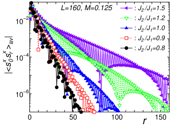
Figure 5: (Color online) Absolute values of the averaged transverse-spin correlation function, $|\langle s^{x}_{0}s^{x}_{r}\rangle_{\rm av}|$, in the antiferromagnetic zigzag ladder with $L=160$ spins for $M=0.125$ and several $J_{2}/J_{1}$.

Let us discuss numerical results. Figure 2(c) shows typical behaviors of the averaged correlation functions in the SDW₂ phase. The longitudinal-spin and two-magnon correlation functions decay algebraically and the former is clearly dominant. By contrast, as shown in Fig. 5, the transverse-spin correlation decays exponentially. This can be seen as evidence for the appearance of two-magnon bound states in this parameter regime. The correlation length of transverse spins becomes larger with increasing $J_{2}/J_{1}$. This is in accordance with the bosonization prediction that the energy gap for the single-spin excitation is generated by the cosine term with the coefficient $g_{1}\sim J_{1}$ for $J_{1}/J_{2}\ll 1$. We have found essentially the same behavior of the correlation functions as shown in Fig. 2(c) for the entire parameter region where the two-spin-flips with $\Delta S^{z}_{\rm tot}=2$ are observed in the magnetization process. After the dominant correlation function and the formation of two-magnon bound pairs, we call this phase the SDW₂ phase.

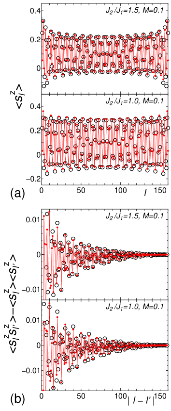
Figure 6: (Color online) Correlation functions in the antiferromagnetic zigzag ladder with $L=160$ spins in the SDW₂ phase; (a) local spin polarization $\langle s^{z}_{l}\rangle$ and (b) longitudinal-spin fluctuation $\langle s^{z}_{l}s^{z}_{l^{\prime}}\rangle-\langle s^{z}_{l}\rangle\langle s^{z}_{l^{\prime}}\rangle$. The upper and lower panels show the results for $(J_{2}/J_{1},M)=(1.5,0.1)$ and $(1.0,0.1)$, respectively. The open symbols represent the DMRG data and the solid symbols are the results of fitting to Eqs. (30) and (31). In (b), the data for $l=L/2-[r/2]$ and $l^{\prime}=L/2+[(r+1)/2]$ are shown as a function of $r=|l-l^{\prime}|$.

In order to estimate the exponent $\eta$ and to further demonstrate the validity of the effective theory for the SDW₂ phase, we fit the DMRG data of the local-spin polarization $\langle s^{z}_{l}\rangle$ and the longitudinal-spin fluctuation $\langle s^{z}_{l}s^{z}_{l^{\prime}}\rangle-\langle s^{z}_{l}\rangle\langle s^{z}_{l^{\prime}}\rangle$ to analytic forms obtained from the bosonization approach. Using Eqs. (21), (26), and (27) and applying the Dirichlet boundary condition in the same manner as in Sec. III, we obtain the correlators for a finite open zigzag ladder as

$$\langle s^{z}_{l}\rangle=\frac{1}{2}-2z(l;\tilde{q}),$$ (30)

$$\langle s^{z}_{l}s^{z}_{l^{\prime}}\rangle-\langle s^{z}_{l}\rangle\langle s^{z}_{l^{\prime}}\rangle=4\left[Z(l,l^{\prime};\tilde{q})-z(l;\tilde{q})z(l^{\prime};\tilde{q})\right],$$ (31)

with

$$\tilde{q}=\frac{2\pi L}{L+1-2\delta}\left(\frac{1}{4}-\frac{M}{2}\right).$$ (32)

In the limit $l\ll L$, Eq. (30) reduces to

$$\langle s^{z}_{l}\rangle=M+\frac{2(-1)^{l}a}{[2(l-\delta)]^{\eta/2}}\sin\left[\left(\frac{\pi}{2}-\pi M\right)(l-\delta)\right],$$ (33)

showing Friedel oscillations with wavenumber $\pi(\frac{1}{2}+M)$.

Figure 6 shows DMRG results and their fits to Eqs. (30) and (31). The results for $J_{2}/J_{1}=1.5$ show that the numerical data at relatively large $J_{2}/J_{1}$ are fitted pretty well by the analytic forms. Note that only three fitting parameters, $\eta$, $a$, and $\delta$, are used in the fitting procedure. For smaller $J_{2}/J_{1}$, the fitting results become less satisfactory, presumably because a smaller value of $\eta$ amplifies effects of both finite system size and higher-order terms omitted in the analytic forms (see also the discussion below for the estimate of $\eta$). Nevertheless the fitting still gives a rather good result at $J_{2}/J_{1}=1.0$ as well. This observation gives a strong support to the validity of the TLL theory for the SDW₂ phase. We emphasize that the successful fitting directly demonstrates that the characteristic wavenumber of the spin-density wave is $Q_{2}=\pm\pi(1/2+M)$, in accordance with the theory above. In the phase diagram in Fig. 1(a), we plot the parameter points where the fitting worked well, which cover almost the entire region of the SDW₂ phase. In the vicinity of the 1/3-plateau, however, good fitting results were not obtained due to the strong boundary effects.

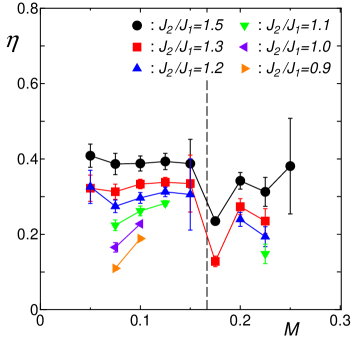
Figure 7: (Color online) $M$ dependence of the exponent $\eta$ for the SDW₂ phase estimated from the fitting of $\langle s^{z}_{l}s^{z}_{l^{\prime}}\rangle-\langle s^{z}_{l}\rangle\langle s^{z}_{l^{\prime}}\rangle$ for the antiferromagnetic zigzag ladder with $L=160$ spins. The error bars represent the difference of the estimates obtained from the fitting of the data of different ranges. The vertical dashed line corresponds to $M=1/6$ where the 1/3-plateau can appear for small $J_{2}/J_{1}$. The exponent $\eta$ relates to the parameter $K_{+}$ as $\eta=K_{+}$ in the TLL theory for the SDW₂ phase.

In Fig. 7, we present the exponent $\eta$ estimated from the fitting of the longitudinal-spin fluctuation $\langle s^{z}_{l}s^{z}_{l^{\prime}}\rangle-\langle s^{z}_{l}\rangle\langle s^{z}_{l^{\prime}}\rangle$. Although the estimates have rather large error bars coming from high sensitivity to the choice of the data range used in the fitting, we can safely conclude that the exponent for $J_{2}/J_{1}\lesssim 1.5$ is always small, i.e., $\eta\lesssim 0.5$. This result reflects the fact that the longitudinal-spin correlation is the strongest in the SDW₂ phase. Furthermore, the data show the tendency that $\eta$ increases with $J_{2}/J_{1}$. Combining this observation with the perturbative result (25) for $J_{2}\gg J_{1}$, we may expect that $\eta$ increases monotonically with $J_{2}/J_{1}$ but less than 1 for the entire regime of $J_{2}/J_{1}\gtrsim 1$. This means that the SDW₂ phase, with the dominant longitudinal-spin correlation, should extend from the intermediate coupling regime of $J_{2}/J_{1}\sim 1$ to the limit $J_{2}/J_{1}\to\infty$.

With decreasing $J_{2}/J_{1}$, the SDW₂ phase appears to touch the 1/3-plateau phase. Here we discuss this plateau-nonplateau transition within the TLL theory for the SDW₂ phase. We can consider the effective Hamiltonian with a three-particle umklapp scattering,

$$\widetilde{\mathcal{H}}^{\prime}_{+}=\widetilde{\mathcal{H}}_{+}+\tilde{\lambda}\int d\bar{x}\sin\left[\pi\bar{x}(6M-1)+3\sqrt{2\pi}\phi_{+}\right],$$ (34)

where $\widetilde{\mathcal{H}}_{+}$ is given in Eq. (27), and $\tilde{\lambda}$ is the coupling constant for three-particle umklapp scattering. The umklapp term becomes uniform only at $M=1/6$. When $M=1/6$, the umklapp term is relevant for $K_{+}<4/9$. Then the $\phi_{+}$ field is pinned and acquires a mass gap. This results in the 1/3-plateau phase with up-up-down spin structure. On the other hand, when approaching the 1/3-plateau from incommensurate magnetization $M\to 1/6$, $K_{+}$ takes the universal value $K_{+}\to 2/9$.Schulz1980 This is a commensurate-incommensurate transition. Figure 7 indicates that the estimated decay exponent $\eta$ at slightly above $M=1/6$ seems smaller than $4/9$ even for $J_{2}/J_{1}=1.5$, suggesting the appearance of the 1/3-plateau at this coupling $J_{2}/J_{1}$. This would mean that the upper critical value of the 1/3-plateau phase is larger than 1.5, $(J_{2}/J_{1})_{\rm p2}>1.5$, which is larger than the previous estimate $(J_{2}/J_{1})_{\rm p2}\sim 1.25$ obtained from magnetization curves.OkunishiT2003 While our estimated values of $\eta$ may contain some large errors, another possible source of this discrepancy is that the analysis of magnetization curves could miss the plateau with an exponentially small width. Further studies with higher accuracy will be needed for resolving this issue.

V 1/3-plateau phase

The 1/3-plateau phase with a finite spin gap emerges at the magnetization $M=1/6$ and for the parameter regime $0.487<J_{2}/J_{1}\lesssim 1.25$.OkunishiT2003 ; OkunishiT2003B ; TonegawaOONK2004 In the 1/3-plateau phase the system has the magnetic LRO of “up-up-down” structure,OkunishiT2003 ; OkunishiT2003B as shown in Fig. 8(a). The ground state is therefore three-fold degenerate in the thermodynamic limit.

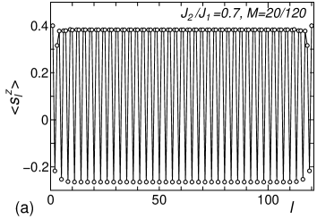
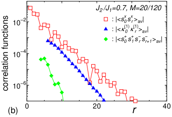
Figure 8: (Color online) (a) Local magnetization $\langle s^{z}_{l}\rangle$ clearly shows the up-up-down spin configuration. (b) Semilog plot of the absolute values of the averaged correlation functions in the antiferromagnetic zigzag ladder with $L=120$ spins for $(J_{2}/J_{1},M)=(0.7,20/120)$.

The analysis of magnetization curves has shown that the 1/3-plateau phase is surrounded by the TLL1 and SDW₂ phases [see Fig. 1 of Ref. OkunishiT2003, and Fig. 1(b) of the present paper]. As we discussed in Secs. III and IV, we can understand this phase diagram as the 1/3-plateau phase emerging from instabilities of three-particle umklapp scattering processes which are inherent in the TLL1 and SDW₂ phases. Here we shall discuss how the up-up-down spin configuration emerges through pinning of bosonic fields.

When $J_{2}/J_{1}$ is small, the plateau emerges from the TLL1 phase. As discussed in Sec. III, the transition is induced by the three-particle umklapp scattering process. If we fix the magnetization at $M=1/6$ and increase $J_{2}/J_{1}$, the umklapp term becomes relevant at $K<2/9$. Indeed we observed $K\simeq 2/9$ at $J_{2}/J_{1}=0.5$ in Fig. 4, which implies that for $J_{2}/J_{1}\gtrsim 0.5$ the 1/3-plateau phase appears. As the umklapp term is relevant, the $\phi$ field is pinned at the bottom of the sine potential in Eq. (20), $\sqrt{4\pi}\langle\phi\rangle=\pi/2$, $7\pi/6$, and $11\pi/6$ ($\lambda>0$). The bosonization formula of $s^{z}_{l}$, Eq. (8), then reduces to

$$s^{z}_{l}\!\! = \!\!\frac{1}{6}-(-1)^{l}a\sin\left(\frac{\pi l}{3}+\sqrt{4\pi}\langle\phi\rangle\right)$$ (35)

$$= \!\!\frac{1}{6}-a\cos\left(\frac{2\pi(l+n)}{3}\right),\quad(n=0,1,2),$$

where $a>0$. Equation (35) gives the up-up-down LRO with three-fold degeneracy in the ground state.LecheminantO2004 ; HidaA2005 ; Notephi

With larger $J_{2}/J_{1}$, the plateau phase is next to the SDW₂ phase. As discussed in Sec. IV, this phase transition is controlled by the three-particle umklapp term, the second term in Eq. (34). When $K_{+}<4/9$ and $M=1/6$, this term becomes relevant, and the $\phi_{+}$ field is pinned to minimize the potential energy. The pinned values are $\sqrt{2\pi}\langle\phi_{+}\rangle=\pi/6$, $5\pi/6$, and $3\pi/2$ ($\tilde{\lambda}<0$). Substituting also $\phi_{-}=\langle\phi_{-}\rangle$ [Eq. (26)] into the bosonized form of $s^{z}_{l}$, Eq. (21), yields

$$s^{z}_{l}=\frac{1}{6}+a\sin\left(\frac{2\pi l}{3}+\sqrt{2\pi}\langle\phi_{+}\rangle\right),$$ (36)

which explains the three-fold-degenerate ground state with the up-up-down LRO.

Since both $\phi_{+}$ and $\phi_{-}$ fields are pinned, all low-energy excitations in the 1/3-plateau phase are gapped. It thus follows that all correlation functions, except the long-ranged longitudinal spin correlation, decay exponentially. Figure 8 shows the averaged correlation functions for $J_{2}/J_{1}=0.7$ and $M=1/6$ as a typical example for the 1/3-plateau phase. The correlation functions decay exponentially in accordance with the theory.

VI Vector chiral phase

The vector chiral phase is characterized by the spontaneous breaking of parity symmetry accompanied by nonvanishing expectation value of the vector chirality, $\langle\kappa_{l}^{(n)}\rangle=\langle({\bm{s}}_{l}\times{\bm{s}}_{l+n})^{z}\rangle\neq 0$. The bosonization theory for the vector chiral phase was developed in Refs. NersesyanGE1998, and KolezhukV2005, , and the appearance of the vector chiral LRO in the zigzag spin ladder (1) has been numerically confirmed recently.McCullochKKKSK2008 ; Okunishi2008 In this section we present results from our detailed numerical study of correlation functions and compare them with their asymptotic forms derived from the bosonization theory.

Let us first briefly summarize the results from the bosonization theory. As discussed in Sec. IV, the effective Hamiltonian (23) describes the zigzag spin ladder (1) in the limit $J_{2}\gg J_{1}$. When the $g_{2}$ term is most relevant, we may employ the mean-field decoupling approximationNersesyanGE1998 in which both $d\theta_{+}/d\bar{x}$ and $\sin(\sqrt{2\pi}\theta_{-})$ are assumed to acquire nonvanishing expectation values to minimize the $g_{2}$ term. The bosonic fields are thus pinned as

$$\langle\theta_{-}\rangle=\mp\sqrt{\frac{\pi}{8}},~{}~{}~{}\left\langle\frac{d\theta_{+}}{d\bar{x}}\right\rangle=\pm\sqrt{\frac{2}{\pi}}c,$$ (37)

where $c$ is a positive constant. Selecting one set of the signs from $(+,-)$ and $(-,+)$ in Eq. (37) corresponds to the spontaneous $Z_{2}$-symmetry breaking in the vector chiral phase. The antisymmetric sector $(\phi_{-},\theta_{-})$ thus acquires an energy gap and the low-energy physics of the phase is governed by the Gaussian model of the $(\phi_{+},\theta_{+})$ fields, Eq. (27), in which the $\theta_{+}$ field has been redefined as $\theta_{+}\to\theta_{+}-\langle d\theta_{+}/d\bar{x}\rangle\bar{x}$ to absorb the nonzero expectation value of $\langle d\theta_{+}/d\bar{x}\rangle$. The vector chiral phase is described by a one-component TLL theory defined by Eqs. (21), (LABEL:eq:s+-boson-twochain), (27), and (37).

Equation (LABEL:eq:s+-boson-twochain) allows us to write the vector chiral operators $\kappa_{l}^{(n)}$ as

$$\kappa_{l}^{(1)}\!\! \sim \!\!\sin(\sqrt{2\pi}\theta_{-}),$$ (38)

$$\kappa_{l}^{(2)}\!\! \sim \!\!\frac{d\theta_{+}}{d\bar{x}}.$$ (39)

The nonvanishing expectation values in Eq. (37) result in the vector chiral LRO in the ground state. We note that the expectation values of the vector chirality satisfy the relation

$$J_{1}\langle\kappa_{l}^{(1)}\rangle+2J_{2}\langle\kappa_{l}^{(2)}\rangle=0,$$ (40)

so that there is no net spin current.HikiharaKMF2008 Furthermore, one can easily obtain the leading asymptotic behaviors of the transverse- and longitudinal-spin correlation functions as follows:

$$\langle s^{x}_{0}s^{x}_{r}\rangle=\frac{\tilde{A}^{x}}{|r|^{1/4K_{+}}}\cos(\widetilde{Q}r)+\cdots,$$ (41)

$$\langle s^{x}_{0}s^{y}_{r}\rangle=\pm\frac{\tilde{A}^{x}}{|r|^{1/4K_{+}}}\sin(\widetilde{Q}r)+\cdots,$$ (42)

$$\langle s^{z}_{0}s^{z}_{r}\rangle=M^{2}-\frac{K_{+}}{\pi^{2}r^{2}}+\cdots,$$ (43)

where $\widetilde{Q}=(\pi+c)/2$, and $\tilde{A}^{x}$ is a positive constant. Equations (41) and (42) indicate that the spin components perpendicular to the applied field have a spiral structure with the incommensurate wavenumber $\widetilde{Q}$, which comes from the finite expectation value of $\langle d\theta_{+}/d\bar{x}\rangle$. This helical quasi-LRO of the transverse components is a characteristic feature of the vector chiral phase. The sign factor $\pm$ in Eq. (42) comes from the sign $\pm$ in Eq. (37), and it defines the chirality, i.e., the direction of the spiral pitch. In the longitudinal-spin correlation function, the oscillating term with wavenumber $Q=\pi(\frac{1}{2}+M)$ decays exponentially as it includes the disordered $\phi_{-}$ field. Therefore, if $1/(4K_{+})<2$, the transverse-spin correlation function is dominant except the long-ranged vector chiral correlations.

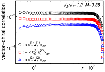
Figure 9: (Color online) Averaged vector chiral correlation functions in the antiferromagnetic zigzag ladder with $L=160$ spins for $(J_{2}/J_{1},M)=(1.2,0.35)$. Open circles, squares, and triangles respectively represent the DMRG data of $\langle\kappa^{(1)}_{0}\kappa^{(1)}_{r}\rangle_{\rm av}$, $-\langle\kappa^{(1)}_{0}\kappa^{(2)}_{r}\rangle_{\rm av}$, and $\langle\kappa^{(2)}_{0}\kappa^{(2)}_{r}\rangle_{\rm av}$, where $\kappa^{(n)}_{r}=\left({\bm{s}}_{r}\times{\bm{s}}_{r+n}\right)^{z}$.

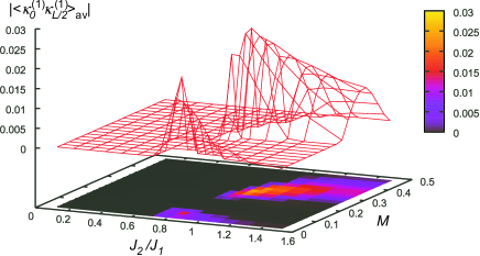
Figure 10: (Color online) Amplitude of the vector chiral correlations at a distance $r=L/2$, $|\langle\kappa^{(1)}_{0}\kappa^{(1)}_{L/2}\rangle_{\rm av}|$, in the antiferromagnetic zigzag ladder with $L=160$ spins.

In Fig. 9, we present our DMRG results of the averaged vector chiral correlation functions $\langle\kappa_{0}^{(n)}\kappa_{r}^{(n^{\prime})}\rangle_{\rm av}$ for $(J_{2}/J_{1},M)=(1.2,0.35)$, a representative point in the vector chiral phase. Clearly, the vector chiral correlations are long-range ordered (the reduction at $r>100$ are due to boundary effects and should be ignored). Figure 10 shows $M$ and $J_{2}/J_{1}$ dependences of the amplitude of the vector chiral correlations measured at distance $r=L/2$, $|\langle\kappa^{(1)}_{0}\kappa^{(1)}_{L/2}\rangle_{\rm av}|$, which indicates the strength of the LRO. This figure shows the parameter regions of the vector chiral phase; the parameter points where we observe the vector chiral LRO are plotted in Fig. 1(b). The vector chiral phase appears when $J_{2}/J_{1}$ is not small, and the phase space is split, by the SDW₂ phase, into two regions with either small or large magnetization $M$. This is in contrast with the $J_{1}$-$J_{2}$ zigzag ladder with ferromagnetic $J_{1}$ and AF $J_{2}$ which has the vector chiral phase only at small $M$.HikiharaKMF2008 ; SudanLL2008 ; LauchliSL2009 It is also important to note that each one of the vector chiral phases is next to a TLL2 phase [see Fig. 1(b)]. The amplitude of the vector chiral order parameter exhibits a steep rise at the boundaries to the SDW₂ and TLL2 phases for small $J_{2}/J_{1}$ (see also Fig. 8 of Ref. McCullochKKKSK2008, for $J_{2}/J_{1}=1$) while the rise is modest for large $J_{2}/J_{1}$. Incidentally, we have numerically confirmed that the vector chiral correlations satisfy the relation (40). These observations on the vector chiral order are consistent with the previous numerical results.McCullochKKKSK2008 ; Okunishi2008

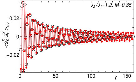
Figure 11: (Color online) Averaged transverse-spin correlation function $\langle s^{x}_{0}s^{x}_{r}\rangle_{\rm av}$ in the antiferromagnetic zigzag ladder with $L=160$ spins for $(J_{2}/J_{1},M)=(1.2,0.35)$. Open circles represent the DMRG data. The fits to Eq. (41) are shown by solid circles.

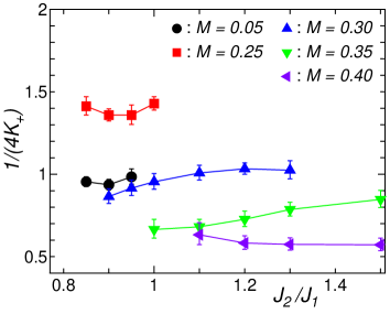
Figure 12: (Color online) $J_{2}/J_{1}$ dependence of the decay exponent $1/(4K_{+})$ of the transverse-spin correlation function $\langle s^{x}_{0}s^{x}_{r}\rangle_{\rm av}$ in the vector chiral phase for the antiferromagnetic zigzag ladder with $L=160$ sites.

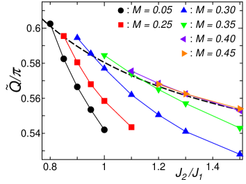
Figure 13: (Color online) $J_{2}/J_{1}$ dependence of the wavenumber $\widetilde{Q}$ of the transverse-spin correlation function $\langle s^{x}_{0}s^{x}_{r}\rangle_{\rm av}$ in the vector chiral phase for the antiferromagnetic zigzag ladder with $L=160$ sites. The dashed curve represents the classical pitch angle $\widetilde{Q}=\arccos(-J_{1}/4J_{2})$.

To estimate the TLL parameter $K_{+}$ and the wavenumber $\tilde{Q}$ of the spiral transverse-spin correlation, we fit the DMRG data of $\langle s^{x}_{0}s^{x}_{r}\rangle_{\rm av}$ in the systems with $L=120$ and $160$ spins to Eq. (41), with taking $\widetilde{Q}$, $K_{+}$, and $\tilde{A}^{x}$ as fitting parameters. Figure 11 shows the result for $(J_{2}/J_{1},M)=(1.2,0.35)$ and $L=160$. We see that the DMRG data are fitted very well to the analytic form, except for large distances $r\gtrsim 100$ where the boundary effect is not negligible. The good agreement between the numerical data and the fits supports the validity of the TLL theory for the vector chiral phase.

The decay exponent $1/(4K_{+})$ of the transverse-spin correlation $\langle s^{x}_{0}s^{x}_{r}\rangle_{\rm av}$ is shown in Fig. 12. We have compared the estimates from $L=160$ and $120$ spins and confirmed that the finite-size effect is negligible in the data shown in the figure but not so for some parameter points (results for which are not shown in Fig. 12) in the very vicinity of the phase boundaries. It turns out that the exponent is rather small, $1/(4K_{+})\lesssim 1$, in most parameter region of the vector chiral phase, suggesting the dominant spiral transverse-spin correlation. The exponent becomes larger, as we move closer to the 1/3-plateau phase.

Figure 13 shows the wavenumber $\widetilde{Q}$ of the transverse-spin correlation function. While $\widetilde{Q}$ almost coincides with the classical pitch angle $\arccos(-J_{1}/4J_{2})$ near the boundary to the TLL2 phase, it becomes smaller than the classical pitch angle with increasing $J_{2}/J_{1}$, i.e., moving inside the vector chiral phase. We thus find that the incommensurate wavenumber $\widetilde{Q}$ in the vector chiral phase is renormalized towards the commensurate value $\pi/2$ due to quantum fluctuations.

VII TLL2 phase

The TLL2 phase is a two-component TLL consisting of two flavors of free bosons. In this section, we develop its effective low-energy theory based on the bosonization of Jordan-Wigner fermions. We then discuss DMRG results, which support the effective theory.

The TLL2 phase is realized in two separated regions of high and low magnetic fields in the magnetic phase diagram. Here we first consider the high-field TLL2 phase, for which the origin of the two bosonic modes can be easily understood by examining the instability of the fully polarized phase.

Inside the fully polarized phase ($h>h_{\mathrm{s}}$), the spin-wave excitation has a finite energy gap and the dispersion relation is given by Eq. (6). As the magnetic field is lowered, the energy gap decreases and vanishes at the saturation field $h=h_{\mathrm{s}}$. For $h<h_{\mathrm{s}}$, the soft magnons proliferate and collectively form a TLL. We notice that there are two distinct cases:

(i) When $J_{2}/J_{1}<1/4$, the bottom of the single-magnon dispersion is at $k=\pi$ (mod $2\pi$). Magnons with $k\approx\pi$ become soft and condense below the saturation field $h_{\mathrm{s}}$, yielding a one-component TLL. Indeed, we have found the TLL1 phase in this case (see Sec. III).

(ii) When $J_{2}/J_{1}>1/4$, the dispersion has two minima, $k=\pi\pm Q_{0}$ with $Q_{0}=\arccos(J_{1}/4J_{2})$. Both magnons with $k=\pi+Q_{0}$ and $\pi-Q_{0}$ become soft and proliferate below the saturation field. The resulting phase is the TLL2 phase which consists of equal densities of two flavors of condensed magnons. We note that, if the densities are not equal, the vector chiral phase will be realized,KolezhukV2005 as we will discuss later.

A similar argument should apply to the TLL2 phase appearing at lower magnetic field. The elementary excitation driving the instability of the dimer ground state is a “spinon,” a domain wall separating two regions of different dimer pattern.ShastryS1981 ; BrehmerKMN1998 ; OkunishiM2001 For $J_{2}/J_{1}<(J_{2}/J_{1})_{\rm L}$, the dispersion of the two-spinon state has a single minimum at $k=\pi$ and only one soft mode is relevant in destabilizing the dimer state. The TLL1 phase is thus expected to show up for $M>0$. For $J_{2}/J_{1}>(J_{2}/J_{1})_{\rm L}$, on the other hand, the two-spinon excitation spectrum exhibits a double-well structure with minima at incommensurate momenta $k=\pm k_{0}$, which leads to the TLL2 (or vector chiral) phase for $M>0$. The critical coupling at which the lowest points deviate from $k=\pi$ has been estimated to be $(J_{2}/J_{1})_{\rm L}=0.54$.OkunishiM2001

VII.1 Two-component TLL theory

In this subsection we describe the two-component TLL theory of the high-field TLL2 phase in detail. As we discussed above, this phase can be understood as a two-component TLL emerging from condensation of two soft magnon modes. This suggests to formulate a low-energy effective theory in terms of interacting magnons.KolezhukV2005 ; UedaTotsuka2009 Such an approach is valid and useful near the saturation field. An alternative approach we adopt here is to formulate the low-energy theory in terms of Jordan-Wigner fermions filling two separate Fermi seas. Advantage of the latter approach is that it can be applied in the whole TLL2 phase. The connection to the magnon picture will also be discussed below.

We apply the Jordan-Wigner transformation

$$s^{z}_{l}\!\! = \!\!\frac{1}{2}-f^{\dagger}_{l}f_{l},$$ (44a)

$$s^{+}_{l}\!\! = \!\!(-1)^{l}f_{l}\exp\left(-i\pi\sum_{n<l}f^{\dagger}_{n}f_{n}\right),$$ (44b)

$$s^{-}_{l}\!\! = \!\!(-1)^{l}f^{\dagger}_{l}\exp\left(i\pi\sum_{n<l}f^{\dagger}_{n}f_{n}\right),$$ (44c)

to rewrite the Hamiltonian (1) in the form $H=H_{0}+H^{\prime}$, where

$$H_{0}\!\! = \!\!-\frac{J_{1}}{2}\sum_{l}\left(f^{\dagger}_{l}f_{l+1}+f^{\dagger}_{l+1}f_{l}\right)$$ (45)

$$\!\!{}+J_{2}M\sum_{l}\left(f^{\dagger}_{l}f_{l+2}+f^{\dagger}_{l+2}f_{l}\right)$$

$$\!\!{}-[2M(J_{1}+J_{2})-h]\sum_{l}f^{\dagger}_{l}f_{l},$$

and

$$H^{\prime}\!\! = \!\!J_{1}\sum_{l}:\!f^{\dagger}_{l}f_{l}\!:\,:\!f^{\dagger}_{l+1}f_{l+1}\!:$$ (46)

$$\!\!{}+J_{2}\sum_{l}\left(:\!f^{\dagger}_{l}f_{l}\!:\,:\!f^{\dagger}_{l+2}f_{l+2}\!:-f^{\dagger}_{l+2}f_{l}:\!f^{\dagger}_{l+1}f_{l+1}\!:\right.$$

$$\hskip 39.83385pt\left.-f^{\dagger}_{l}f_{l+2}:\!f^{\dagger}_{l+1}f_{l+1}\!:\right).$$

Here $:\!X\!:$ denotes normal ordering of $X$ with respect to the filled Fermi sea of fermions with the dispersion

$$E(k)=-J_{1}\cos k+2J_{2}M\cos(2k)-2M(J_{1}+J_{2})+h,$$ (47)

determined from Eq. (45). Note that the wave number $k$ is measured from $\pi$ as the $(-1)^{l}$ factor is included in the Jordan-Wigner transformation. As discussed above, in the TLL2 phase the dispersion has two minima and, accordingly, there are four Fermi points located at $k=\pm k_{s}$, $\pm k_{l}$ ($k_{s}<k_{l}$, see Fig. 14). The density of fermions is

$$\rho=\frac{1}{\pi}(k_{l}-k_{s})=\frac{1}{2}-M.$$ (48)

In the limit $M\to\frac{1}{2}$, both $k_{l}$ and $k_{s}$ approach $Q_{0}$. Introducing slowly-varying fermionic fields for each Fermi point, we write the fermion annihilation operator as

$$f_{j}\!\! = \!\!e^{ik_{l}x}\psi_{lR}(x)+e^{-ik_{l}x}\psi_{lL}(x)$$ (49)

$$\!\!{}+e^{ik_{s}x}\psi_{sL}(x)+e^{-ik_{s}x}\psi_{sR}(x),$$

where the continuous variable $x$ is identified with lattice index $j$. We linearize the dispersion around the four Fermi points and replace $H_{0}$ with

$$\widetilde{H}_{0}\!\! = \!\!iv_{l}\int dx\left(\psi^{\dagger}_{lL}\frac{d}{dx}\psi_{lL}-\psi^{\dagger}_{lR}\frac{d}{dx}\psi_{lR}\right)$$ (50)

$$\!\!\!{}+iv_{s}\int dx\left(\psi^{\dagger}_{sL}\frac{d}{dx}\psi_{sL}-\psi^{\dagger}_{sR}\frac{d}{dx}\psi_{sR}\right),$$

where the velocities $v_{l}$ and $v_{s}$ are in general different. The linearized kinetic term can be written as

$$\widetilde{H}_{0}=\sum_{\nu=l,s}\frac{v_{\nu}}{4\pi}\int dx\left[\left(\frac{d\varphi_{\nu L}}{dx}\right)^{2}+\left(\frac{d\varphi_{\nu R}}{dx}\right)^{2}\right]$$ (51)

in terms of the chiral bosonic fields $\varphi_{\nu L}$ and $\varphi_{\nu R}$, which obey the commutation relations

$$\begin{split}&[\varphi_{\nu R}(x),\varphi_{\nu R}(y)]=i\pi\mathrm{sgn}(x-y),\\ &[\varphi_{\nu L}(x),\varphi_{\nu L}(y)]=-i\pi\mathrm{sgn}(x-y),\\ &[\varphi_{\nu R}(x),\varphi_{\nu^{\prime}L}(y)]=-i\pi\delta_{\nu,\nu^{\prime}}.\end{split}$$ (52)

The fermion densities are written as

$$\begin{split}\rho_{\nu R}(x)&=\;:\!\psi^{\dagger}_{\nu R}(x)\psi_{\nu R}(x)\!:\;=\frac{1}{2\pi}\frac{d\varphi_{\nu R}}{dx},\\ \rho_{\nu L}(x)&=\;:\!\psi^{\dagger}_{\nu L}(x)\psi_{\nu L}(x)\!:\;=\frac{1}{2\pi}\frac{d\varphi_{\nu L}}{dx}.\end{split}$$ (53)

Finally, the slowly-varying fermionic fields are bosonized,

$$\begin{split}\psi_{\nu R}(x)&=\frac{\eta_{\nu}}{\sqrt{2\pi\alpha}}e^{i\varphi_{\nu R}(x)},\\ \psi_{\nu L}(x)&=\frac{\eta_{\nu}}{\sqrt{2\pi\alpha}}e^{-i\varphi_{\nu L}(x)},\end{split}$$ (54)

where $\alpha$ is a short-distance cutoff on the order of the lattice spacing, and $\eta_{\nu}$ are the Klein factors obeying $\{\eta_{\nu},\eta_{\nu^{\prime}}\}=2\delta_{\nu,\nu^{\prime}}$.

Figure 14: Four Fermi points located at $k=\pm k_{s}$ and $\pm k_{l}$. The density of fermions is related to the magnetization, $k_{l}-k_{s}=\pi(\frac{1}{2}-M)$. The phase transition to the TLL1 phase occurs when $k_{s}=0$, i.e., when the inner two Fermi points merge at $k=0$.

The interaction Hamiltonian $H^{\prime}$ gives rise to various scattering processes of fermionic fields $\psi_{\nu L/R}$. Among all, important in the TLL2 phase are (short-range) density-density interactions,

$$H_{\rho}\!\! = \!\!\pi\!\int\!\!dx\{2g_{2l}\rho_{lL}(x)\rho_{lR}(x)+2g_{2s}\rho_{sL}(x)\rho_{sR}(x)$$

$${}\hskip 19.91692pt+2g_{2\perp}[\rho_{lL}(x)\rho_{sR}(x)+\rho_{lR}(x)\rho_{sL}(x)]$$

$${}\hskip 19.91692pt+g_{4l}[\rho_{lL}(x)\rho_{lL}(x)+\rho_{lR}(x)\rho_{lR}(x)]$$

$${}\hskip 19.91692pt+g_{4s}[\rho_{sL}(x)\rho_{sL}(x)+\rho_{sR}(x)\rho_{sR}(x)]$$

$${}\hskip 19.91692pt+2g_{4\perp}[\rho_{lL}(x)\rho_{sL}(x)+\rho_{lR}(x)\rho_{sR}(x)]\},$$

where $g_{2l/s}$, $g_{2\perp}$, $g_{4l/s}$, and $g_{4\perp}$ are coupling constants that depend on $J_{1}$, $J_{2}$, and $M$. We define the phase fields ($\nu=l,s$)

$$\begin{split}&\phi_{\nu}(x)=\frac{1}{\sqrt{4\pi}}[\varphi_{\nu L}(x)+\varphi_{\nu R}(x)],\\ &\theta_{\nu}(x)=\frac{1}{\sqrt{4\pi}}[\varphi_{\nu L}(x)-\varphi_{\nu R}(x)].\end{split}$$ (56)

The effective Hamiltonian $H_{2}=\widetilde{H}_{0}+H_{\rho}$ is then quadratic in $\phi_{\nu}$ and $\theta_{\nu}$, and is diagonalized as

$$H_{2}=\int dx\sum_{\mu=\pm}\frac{v_{\mu}}{2}\left[\left(\frac{d\theta_{\mu}}{dx}\right)^{2}+\left(\frac{d\phi_{\mu}}{dx}\right)^{2}\right]$$ (57)

by the new fields $\theta_{\pm}$ and $\phi_{\pm}$ which are linearly related to $\theta_{l,s}$ and $\phi_{l,s}$ by

$$\begin{pmatrix}\phi_{l}\\ \phi_{s}\end{pmatrix}=A^{T}\begin{pmatrix}\phi_{+}\\ \phi_{-}\end{pmatrix},\qquad\begin{pmatrix}\theta_{l}\\ \theta_{s}\end{pmatrix}=A^{-1}\begin{pmatrix}\theta_{+}\\ \theta_{-}\end{pmatrix}.$$ (58)

Here the $2\times 2$ matrix

$$A=\begin{pmatrix}A_{11}&A_{12}\\ A_{21}&A_{22}\\ \end{pmatrix}$$ (59)

is a function of the velocities $v_{l,s}$ and the coupling constants $g$’s, whose functional form can be found in Ref. Hikihara05, . Without loss of generality, we can assume $v_{+}>v_{-}$.

The Hamiltonian $H_{2}$ (57) is the low-energy effective theory of the TLL2 phase. It consists of two free bosonic sectors $(\phi_{+},\theta_{+})$ and $(\phi_{-},\theta_{-})$. Other interactions which are not included in $H_{\rho}$ are irrelevant perturbations to $H_{2}$ in the TLL2 phase. An important example of such interactions is the backward-scattering interaction

$$H_{b}\!\! = \!\!g_{1\perp}\int dx\left[\psi^{\dagger}_{sL}(x)\psi^{\dagger}_{sR}(x)\psi_{lL}(x)\psi_{lR}(x)+\mathrm{H.c.}\right]$$ (60)

$$= \!\!-\frac{g_{1\perp}}{2\pi^{2}\alpha^{2}}\int dx\cos[\sqrt{4\pi}(\theta_{l}-\theta_{s})].$$

The irrelevance of the operator $\cos[\sqrt{4\pi}(\theta_{l}-\theta_{s})]$ imposes the condition

$$\frac{1}{(\mathrm{det}\,A)^{2}}[(A_{11}+A_{12})^{2}+(A_{21}+A_{22})^{2}]>2.$$ (61)

We note that the vertex operators $\exp(\pm i\sqrt{4\pi}\phi_{\pm})$ and $\exp(\pm i\sqrt{4\pi}\theta_{\pm})$ have scaling dimension 1.

The matrix $A$ takes a simple form

$$A=\frac{1}{\sqrt{2}}\begin{pmatrix}\sqrt{K_{+}}&0\\ 0&\sqrt{K_{-}}\end{pmatrix}\begin{pmatrix}1&1\\ 1&-1\end{pmatrix},$$ (62)

when the two conditions

$$v_{l}+g_{4l}=v_{s}+g_{4s}\;=:v+g_{4},$$ (63a)

$$g_{2l}=g_{2s}\;=:g_{2},$$ (63b)

are satisfied. In this case, the TLL parameters $K_{\pm}$ and the renormalized velocities $v_{\pm}$ are given by

$$K_{\pm}=\left(\frac{v+g_{4}\pm g_{4\perp}-g_{2}\mp g_{2\perp}}{v+g_{4}\pm g_{4\perp}+g_{2}\pm g_{2\perp}}\right)^{1/2},$$ (64a)

$$v_{\pm}=\left[(v+g_{4}\pm g_{4\perp})^{2}-(g_{2}\pm g_{2\perp})^{2}\right]^{1/2}.$$ (64b)

This simplified effective theory is applicable when $J_{2}/J_{1}\gg 1/4$ and $|M-\frac{1}{2}|\ll\frac{1}{2}$, i.e., when the magnon density is very low and $k_{l}-k_{s}\ll k_{s}$. In this case one can build an effective theory by treating magnons with $k=\pi\pm Q_{0}$ as interacting hard-core bosons.KolezhukV2005 ; UedaTotsuka2009 We adopt a phenomenological effective Hamiltonian of interacting bosons ($0<v<u$),Cazalilla

$$H_{\mathrm{B}}\!\!\! = \!\!\!\int dx\biggl{[}\frac{1}{2m}\biggl{(}\frac{d\psi_{+}^{\dagger}}{dx}\frac{d\psi_{+}}{dx}+\frac{d\psi_{-}^{\dagger}}{dx}\frac{d\psi_{-}}{dx}\biggr{)}$$

$$\hskip 14.22636pt{}+u\bigl{\{}[\rho_{+}(x)]^{2}+[\rho_{-}(x)]^{2}\bigr{\}}+2v\rho_{+}(x)\rho_{-}(x)\biggr{]},$$

where $\psi_{\pm}(x)$ are field operators of two flavors of magnons satisfying $[\psi_{\mu}(x),\psi^{\dagger}_{\mu^{\prime}}(y)]=\delta_{\mu,\mu^{\prime}}\delta(x-y)$, magnon density fluctuations $\rho_{\pm}(x)=\psi^{\dagger}_{\pm}(x)\psi_{\pm}(x)-\rho/2$, and $m$ is their effective mass. The boson density (per flavor) is assumed to be $\rho/2$, where $\rho$ is defined in Eq. (48). In the low-energy, hydrodynamic limit,Haldane1981 ; Giamarchi-text the magnon fields and density fluctuations are written as

$$\psi_{\pm}(x)\sim\sqrt{\frac{\rho}{2}}e^{i\vartheta_{\pm}(x)}+\ldots,$$ (66a)

$$\rho_{\pm}(x)\sim\frac{1}{\pi}\frac{d\varphi_{\pm}(x)}{dx}+\rho\cos[\pi\rho x\!+\!2\varphi_{\pm}(x)]+\ldots,\qquad$$ (66b)

where the phase fields obey $[\varphi_{\mu}(x),\partial_{y}\vartheta_{\mu^{\prime}}(y)]=i\pi\delta_{\mu,\mu^{\prime}}\delta(x-y)$. Substituting (66) into (LABEL:BosonHamiltonian) yields

$$H_{\mathrm{B}}\!\!\! = \!\!\!\int\!dx\biggl{\{}\frac{\rho}{4m}\left[\left(\frac{d\vartheta_{+}}{dx}\right)^{2}+\left(\frac{d\vartheta_{-}}{dx}\right)^{2}\right]$$ (67)

$$\hskip 17.07164pt{}+\frac{u}{\pi^{2}}\left[\left(\frac{d\varphi_{+}}{dx}\right)^{2}+\left(\frac{d\varphi_{-}}{dx}\right)^{2}\right]$$

$$\hskip 17.07164pt{}+\frac{2v}{\pi^{2}}\frac{d\varphi_{+}}{dx}\frac{d\varphi_{-}}{dx}+v\rho^{2}\cos[2(\varphi_{+}\!-\!\varphi_{-})]\biggr{\}}.\qquad$$

Once we make the identification of the phase fields,

$$\varphi_{+}=\frac{1}{2}(\varphi_{sL}+\varphi_{lR}),\qquad\vartheta_{+}=\frac{1}{2}(\varphi_{sL}-\varphi_{lR}),$$ (68a)

$$\varphi_{-}=\frac{1}{2}(\varphi_{lL}+\varphi_{sR}),\qquad\vartheta_{-}=\frac{1}{2}(\varphi_{lL}-\varphi_{sR}),\qquad$$ (68b)

we can readily see that the Hamiltonian (67) is a special case of $\widetilde{H}_{0}+H_{\rho}+H_{b}$, with the coupling constants,

$$v_{l}+g_{4l}=v_{s}+g_{4s}=\frac{\pi\rho}{4m}+\frac{u}{\pi},$$ (69a)

$$g_{2l}=g_{2s}=g_{4\perp}=\frac{v}{\pi},$$ (69b)

$$g_{2\perp}=-\frac{\pi\rho}{4m}+\frac{u}{\pi}.$$ (69c)

Substituting (69) into (64), we find

$$v_{\pm}=\sqrt{\frac{\rho}{m}(u\pm v)},\qquad\left(K_{\pm}\right)^{\pm 1}=\frac{\pi}{2}\sqrt{\frac{\rho}{m(u\pm v)}}.$$ (70)

Note that $v_{-}$ and $K_{-}$ vanish when $u=v$. This corresponds to the instability to the vector chiral order.KolezhukV2005 ; UedaTotsuka2009 ; Cazalilla ; Kolezhuk09 We emphasize again that the bosonic approach described here is applicable only when $\frac{1}{2}-M\ll 1$ and $J_{2}/J_{1}\gg 1/4$, while the general theory (57)–(58) should be valid as a low-energy theory in the whole TLL2 phase.

Next we express the spin operators $\bm{s}_{l}$ using the phase fields in the fermionic formulation. We first rewrite the string operator used in the Jordan-Wigner transformation,

$$\begin{split}\exp\!\left(\!i\pi\sum_{n<l}f^{\dagger}_{n}f_{n}\!\right)\!=&\,e^{i(k_{l}-k_{s})x+i\sqrt{\pi}[\phi_{l}(x^{-})+\phi_{s}(x^{-})]}\\ &+e^{-i(k_{l}-k_{s})x-i\sqrt{\pi}[\phi_{l}(x^{-})+\phi_{s}(x^{-})]},\end{split}$$ (71)

where $x^{-}=x-0^{+}$, and the second term is added to ensure the Hermiticity of the string operator. From Eqs. (44c), (49) (54), and (71), we obtain

$$s^{-}_{l}\!\! = \!\!(-1)^{x}\eta_{s}e^{i\sqrt{\pi}\theta_{s}(x)}\cos[k_{l}x+\sqrt{\pi}\phi_{l}(x)]$$ (72)

$$\!\!\!\!{}+(-1)^{x}\eta_{l}e^{i\sqrt{\pi}\theta_{l}(x)}\cos[-k_{s}x+\sqrt{\pi}\phi_{s}(x)]$$

$$\!\!\!\!{}+(-1)^{x}\eta_{s}e^{i\sqrt{\pi}\theta_{s}}\cos[(k_{l}-2k_{s})x+\!\sqrt{\pi}(\phi_{l}+2\phi_{s})]$$

$$\!\!\!{}+(-1)^{x}\eta_{l}e^{i\sqrt{\pi}\theta_{l}}\cos[(2k_{l}-k_{s})x+\!\sqrt{\pi}(2\phi_{l}+\phi_{s})]$$

$$\!\!\!{}+\ldots,$$

where numerical coefficients are suppressed for simplicity. The transverse correlation function becomes

$$\langle s^{+}_{0}s^{-}_{r}\rangle=\frac{(-1)^{r}c_{l}}{|r|^{x_{l}}}\cos(k_{l}r)+\frac{(-1)^{r}c_{s}}{|r|^{x_{s}}}\cos(k_{s}r)+\ldots,$$ (73)

where $c_{l}$ and $c_{s}$ are constants, and the exponents are given by

$$\begin{split}&x_{l}=\frac{1}{2}(A_{11}^{2}+A_{21}^{2})\left[1+\frac{1}{(\mathrm{det}\,A)^{2}}\right],\\ &x_{s}=\frac{1}{2}(A_{12}^{2}+A_{22}^{2})\left[1+\frac{1}{(\mathrm{det}\,A)^{2}}\right].\end{split}$$ (74)

It follows from $s^{z}_{l}=\frac{1}{2}-s^{-}_{l}s^{+}_{l}$ that

$$s^{z}_{l}\!\! = \!\!M-\frac{1}{\sqrt{\pi}}\frac{d}{dx}(\phi_{l}+\phi_{s})$$ (75)

$$\!\!\!\!{}+c_{1}\sin(2k_{l}x+\sqrt{4\pi}\phi_{l})+c_{2}\sin(-2k_{s}x+\sqrt{4\pi}\phi_{s})$$

$$\!\!\!\!{}+c_{3}\cos[(k_{l}-k_{s})x+\sqrt{\pi}(\phi_{l}+\phi_{s})]\sin[\sqrt{\pi}(\theta_{l}-\theta_{s})]$$

$$\!\!\!\!{}+c_{4}\cos[(k_{l}+k_{s})x+\sqrt{\pi}(\phi_{l}-\phi_{s})]\sin[\sqrt{\pi}(\theta_{l}-\theta_{s})]$$

$$\!\!\!\!{}+c_{5}\cos[2(k_{l}-k_{s})x+\sqrt{4\pi}(\phi_{l}+\phi_{s})]$$

$$\!\!\!\!{}+c_{6}\cos[2(2k_{l}-k_{s})x+\sqrt{4\pi}(2\phi_{l}+\phi_{s})]+\ldots,$$

where $c_{j}$’s are nonuniversal constants. The long-distance behavior of the longitudinal spin correlation is then obtained as

$$\langle s^{z}_{0}s^{z}_{r}\rangle\!\! = \!\!M^{2}-\frac{1}{2\pi^{2}r^{2}}[(A_{11}+A_{12})^{2}+(A_{21}+A_{22})^{2}]$$ (76)

$$\!\!\!{}+\frac{C_{1}}{|r|^{x_{1}}}\cos(2k_{l}r)+\frac{C_{2}}{|r|^{x_{2}}}\cos(2k_{s}r)$$

$$\!\!\!{}+\frac{C_{3}}{|r|^{x_{3}}}\cos[(k_{l}-k_{s})r]+\frac{C_{4}}{|r|^{x_{4}}}\cos[(k_{l}+k_{s})r]$$

$$\!\!\!{}+\frac{C_{5}}{|r|^{x_{5}}}\cos[2(k_{l}-k_{s})r]+\frac{C_{6}}{|r|^{x_{6}}}\cos[2(2k_{l}-k_{s})r]$$

$$\!\!\!{}+\ldots,$$

where $C_{j}$’s are constants, and the exponents are given by

$$x_{1}\!\! = \!\!2(A_{11}^{2}+A_{21}^{2}),\qquad x_{2}=2(A_{12}^{2}+A_{22}^{2}),$$

$$x_{3}\!\! = \!\!\frac{1}{2}[(A_{11}+A_{12})^{2}+(A_{21}+A_{22})^{2}]\left[1+\frac{1}{(\mathrm{det}\,A)^{2}}\right],$$

$$x_{4}\!\! = \!\!\frac{1}{2}[(A_{11}-A_{12})^{2}+(A_{21}-A_{22})^{2}]$$

$$\!\!\!{}+\frac{1}{2(\mathrm{det}\,A)^{2}}[(A_{11}+A_{12})^{2}+(A_{21}+A_{22})^{2}],$$

$$x_{5}\!\! = \!\!2[(A_{11}+A_{12})^{2}+(A_{21}+A_{22})^{2}],$$

$$x_{6}\!\! = \!\!2[(2A_{11}+A_{12})^{2}+(2A_{21}+A_{22})^{2}].$$ (77)

Finally, let us consider local spin polarization $\langle s^{z}_{l}\rangle$ near an open boundary of a semi-infinite spin ladder defined on the sites $l>0$. Assuming the Dirichlet boundary conditions $\phi_{l}(0)=\phi_{s}(0)=0$ as in the TLL1 phase [see Eq. (15)], we obtain

$$\langle s^{z}_{l}\rangle\!\!\! = \!\!\!M+\frac{c_{1}}{(2l)^{x_{1}/2}}\sin(2k_{l}l)-\frac{c_{2}}{(2l)^{x_{2}/2}}\sin(2k_{s}l)$$ (78)

$$\!\!\!{}+\frac{c_{5}}{(2l)^{x_{5}/2}}\cos[2(k_{l}-k_{s})l]$$

$$\!\!\!{}+\frac{c_{6}}{(2l)^{x_{6}/2}}\cos[2(2k_{l}-k_{s})l]+\ldots.$$

Observe that the exponents in Eq. (78) are a half of the corresponding ones in Eq. (76) and that the vertex operators of the $\theta_{l,s}$ fields do not contribute to Eq. (78).

An important characteristic feature of the spin correlations (73) and (76) in the TLL2 phase is the presence of two incommensurate (Fermi) wave numbers $k_{l}$ and $k_{s}$ (and their linear combinations).

Before closing this subsection, we note that Frahm and Rödenbeck studied an exactly solvable zigzag spin ladder model with additional three-spin interactions.FrahmR1997 ; FrahmR1999 Their model has a phase corresponding to our TLL2 phase. They have calculated, using the Bethe ansatz solution and conformal field theory, exponents of several terms in the longitudinal spin correlation (76).

VII.2 Instabilities

In the magnetic phase diagram (Fig. 1) each TLL2 phase is next to a vector chiral phase and the TLL1 phase. Since these neighboring phases are one-component TLLs, one of the two massless modes in the low-energy Hamiltonian (57) has to become massive or disappear from low-energy spectra at the transitions from the TLL2 phase. Here we discuss instabilities of gapless modes in the TLL2 phases which cause the phase transitions to the vector chiral and TLL1 phases.

As pointed out by Kolezhuk and Vekua,KolezhukV2005 in the interacting magnon picture valid in the vicinity of the saturation field [Eqs. (LABEL:BosonHamiltonian)–(70)], the instability to the vector chiral phase corresponds to the “demixing” or “phase separation” instability,Cazalilla ; Kolezhuk09 which occurs when both $v_{-}$ and $K_{-}$ vanish. Alternatively, if we regard the two flavors as up and down pseudospins, the TLL2 and vector chiral phases correspond to paramagnetic and ferromagnetic phases, respectively. The transition between the TLL2 and vector chiral phases is then regarded as a ferromagnetic transition.KunYang Away from the saturation field, the interacting magnon picture is no longer applicable, and we should use the low-energy effective Hamiltonian (57) with the $A$ matrix (59). The instability to the vector chiral phase is then signaled by $v_{-}=0$ and $\mathrm{det}\,A=0$.

The transition between the TLL2 and TLL1 phases is characterized by a cusp singularity in the magnetization curve.OkunishiT2003 Since $M$ and $h$ correspond to the particle density and the chemical potential of the Jordan-Wigner fermions, the origin of the cusp singularity can be attributed to the van Hove singularity of the fermion density of states, which exists at the saddle point $k=0$ of the dispersion (47). Thus, the TLL2-TLL1 transition is considered to occur when the chemical potential matches the saddle-point energy, and the two Fermi seas merge into a single Fermi sea.OkunishiHA1999 Indeed, the Bethe-ansatz study of a solvable model finds that the transition of commensurate-incommensurate type occurs when $k_{s}=0$.FrahmR1997 ; FrahmR1999 In our low-energy effective theory, the transition is driven by the operator (the $c_{2}$ term in $s_{l}^{z}$),

$$\tilde{h}\int dx\sin(-2k_{s}x+\sqrt{4\pi}\phi_{s}),$$ (79)

which turns into a mass term (scaling dimension 1) for fermions at the TLL2-TLL1 transition. Comparison of our effective theory with the Bethe-ansatz study in Ref. FrahmR1999, shows that the $A$ matrix takes the form

$$A=\begin{pmatrix}\xi(\Lambda_{2})&0\\ -1+\xi(0)&1\end{pmatrix},$$ (80)

at the transition ($h\searrow h_{\mathrm{c1}}$), in agreement with our picture of the TLL2-TLL1 transition as a commensurate-incommensurate transition caused by the operator (79). Here $\xi$ is the dressed charge defined in Ref. FrahmR1999, .

VII.3 Numerical results

In Fig. 2(e) we have shown the correlation functions at $J_{2}/J_{1}=0.6$ and $M=0.4$, as a typical example of the TLL2 phase. We see that both the longitudinal- and transverse-spin correlation functions decay algebraically. The vector chiral LRO is clearly absent.

As we have discussed in Sec. VII.1, the defining feature of the TLL2 phase is that its low-energy physics is governed by the two independent sets of free bosons. The low-energy theory is a conformal field theory with central charge $c=1+1$. The central charge can be numerically measured through the entanglement entropy,

$$S(l)=-\mathrm{Tr}_{\Omega}\left[\rho(l)\ln\rho(l)\right],$$ (81)

where the reduced density matrix for the subsystem $\Omega=\{\bm{s}_{j}|\,1\leq j\leq l\}$ is defined by

$$\rho(l)=\mathrm{Tr}_{\bar{\Omega}}|0\rangle\langle 0|.$$ (82)

Here $|0\rangle$ is the ground state wave function, and the spins $\bm{s}_{l+1},\ldots,\bm{s}_{L}$ in the environment $\bar{\Omega}$ are traced out. The entanglement entropy of a 1D critical system with open boundaries is known to have a logarithmic dependence on $l$,Holzhey ; Vidal ; Calabrese

$$S(l)=\frac{c}{6}\ln l+\mathrm{const.},$$ (83)

in the thermodynamic limit, $L\to\infty$ and $l\gg 1$. For finite-size systems of $L$ spins, $\ln l$ in Eq. (83) should be replaced byCalabrese

$$x=\ln\left[\frac{L}{\pi}\sin\left(\frac{\pi l}{L}\right)\right].$$ (84)

Hence we can measure the central charge $c$ as a coefficient of $x$. This method was recently used to detect the central charge of the critical spin Bose metal phase in a related model of the $J_{1}$-$J_{2}$ zigzag ladder with a ring exchange interaction.Sheng2009 Figure 15(a) shows the entanglement entropy $S(l)$ in the TLL2 phase ($J_{2}/J_{1}=0.6$, $M=0.4$) as a function of $x$. We clearly see that $S(l)\sim x/3$, indicating that $c=2$. For comparison, we have computed the entanglement entropy in the TLL1 and vector chiral phases. The numerical results shown in Fig. 15(b) demonstrate that $S(l)\sim x/6$ for large $x$, i.e., $c=1$.

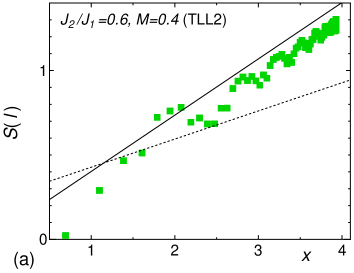
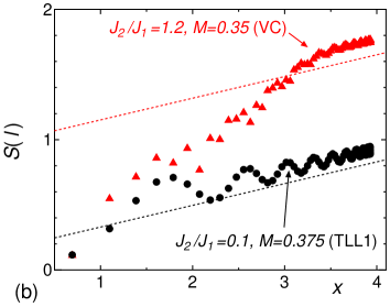
Figure 15: (Color online) (a) Entanglement entropy of the TLL2 phase ($J_{2}/J_{1}=0.6$, $M=0.4$). The horizontal axis is $x=\ln[(L/\pi)\sin(\pi l/L)]$. Solid and dotted lines represent the slope $1/3$ ($c=2$) and $1/6$ ($c=1$), respectively. (b) Entanglement entropy of the TLL1 phase ($J_{2}/J_{1}=0.1$, $M=0.375$) and the vector chiral phase ($J_{2}/J_{1}=1.2$, $M=0.35$). Dotted lines indicate the slope $1/6$ ($c=1$).

Having confirmed that the TLL2 phase has $c=2$, i.e., that the low-energy physics is governed by two free boson theories, we now discuss spin correlation functions. It turned out, however, that the presence of the two Fermi wavenumbers $k_{l}$ and $k_{s}$ makes it difficult to analyze correlation functions in the TLL2 phase. For this reason we focus attention to the simplest, one-point function $\langle s^{z}_{l}\rangle$. The Friedel oscillations near open boundaries give us information on the Fermi wavenumbers.

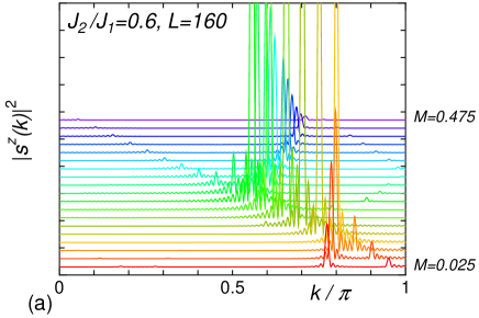
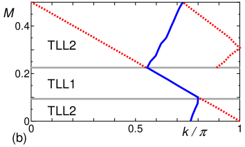
Figure 16: (Color online) (a) Squared modulus of the Fourier transform of the local spin polarization, $|s^{z}(k)|^{2}$, for the antiferromagnetic zigzag ladder with $L=160$ spins and $J_{2}/J_{1}=0.6$. (b) $M$ dependence of peak positions of $|s^{z}(k)|^{2}$. Solid line represents the highest peak while the dotted lines correspond to the subdominant peaks in TLL2 phase. Gray horizontal lines show phase boundaries.

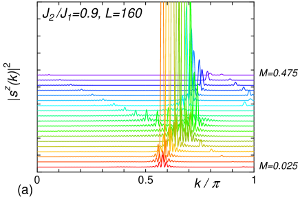
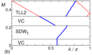
Figure 17: (Color online) (a) Squared modulus of the Fourier transform of the local spin polarization, $|s^{z}(k)|^{2}$, for the antiferromagnetic zigzag ladder with $L=160$ spins and $J_{2}/J_{1}=0.9$. (b) $M$ dependence of peak positions of $|s^{z}(k)|^{2}$. Solid line represents the highest peak while the dotted lines correspond to the subdominant peaks in TLL2 phase. Gray horizontal lines show phase boundaries.

We show in Figs. 16 and 17 the squared modulus of the Fourier transform of the local spin polarization

$$s^{z}(k)=\frac{1}{\sqrt{L}}\sum^{L}_{l=1}e^{ikl}(\langle s^{z}_{l}\rangle-M).$$ (85)

At $J_{2}/J_{1}=0.6$ (Fig. 16) the TLL2 phases appear when $0<M\lesssim 0.075$ and $0.25\lesssim M<1/2$, and the TLL1 phase is located at $0.1\lesssim M\lesssim 0.2$. In the TLL1 phase we see a very sharp peak in $|s^{z}(k)|^{2}$ at $k=\pi(1-2M)$, in agreement with Eq. (15). Although greatly reduced in magnitude, the peak persists in the TLL2 phases. This faint peak comes from the fourth term, with wavenumber $2(k_{l}-k_{s})$, in Eq. (78). We attribute the strongest peak of $|s^{z}(k)|^{2}$ in the TLL2 phase to the second term in Eq. (78) with wavenumber $2k_{l}$. The two peaks meet when the TLL2 phase is turned into the TLL1 phase, i.e., when $k_{s}$ vanishes, in accordance with the discussion in Sec. VII.2. Moreover, at the saturation limit $M\to 1/2$, the wavenumber $k_{\max}$ of the strongest peak approaches $2Q_{0}=2\arccos(J_{1}/4J_{2})$, where $Q_{0}$ is the momentum of the soft magnon in the fully polarized state, while $k_{\max}\to 2k_{0}$ as $M\to 0$, where $k_{0}$ is the momentum of the soft single-spinon excitation in the dimer phase estimated numerically.OkunishiM2001 In the higher-field TLL2 phase we see a third, faint peak, whose wavenumber $k_{3}$ equals $2Q_{0}$ at $M\to 1/2$ and increases with decreasing $M$. We have found numerically that $k_{3}-k_{\max}$ equals $2(k_{l}-k_{s})=\pi(1-2M)$ modulo $2\pi$, from which we conclude $k_{3}=4k_{l}-2k_{s}$. Interestingly, $|s^{z}(k)|^{2}$ does not have a peak corresponding to $k=2k_{s}$. Comparing the peak heights, we can deduce the following inequalities for exponents,

$$x_{1}<x_{5},x_{6}<x_{2},x_{3},x_{4}.$$ (86)

From the relation $x_{l}/x_{s}=x_{1}/x_{2}$, we can also obtain

$$x_{l}<x_{s}.$$ (87)

These observations suggest that the dominant component in the transverse-spin correlation function comes from the first term in Eq. (73) with a wavenumber $\pi\pm k_{l}$ while the dominant longitudinal-spin correlation comes from the third term in Eq. (76) with a wavenumber $2k_{l}$.

Figure 17 shows $|s^{z}(k)|^{2}$ at $J_{2}/J_{1}=0.9$. In this case we have the TLL2 phase for $0.35\lesssim M<1/2$, the SDW₂ phase for $0.075\lesssim M\lesssim 0.2$, and the vector chiral phase for $0<M<0.05$ and $0.2\lesssim M\lesssim 0.3$. Characteristics of incommensurate wavenumbers giving rise to the peaks in $|s^{z}(k)|^{2}$ in the TLL2 phase are the same as in Fig. 16. In the SDW₂ phase the strong peak is found to be at $k=\pi(1/2+M)$, in agreement with Eq. (33).

VIII Concluding remarks

By the thorough comparison between numerically obtained correlation functions and asymptotic behaviors derived from low-energy effective theories, we have identified the nature of critical TLL phases that appear in the spin-1/2 $J_{1}$-$J_{2}$ AF Heisenberg zigzag ladder under magnetic field. These critical phases consist of three one-component TLL phases (the TLL1, SDW₂, and vector chiral phases) and a two-component TLL phase, the TLL2 phase. From the fitting, we numerically estimated the TLL parameter in one-component TLL phases as a function of $J_{2}/J_{1}$ and the magnetization $M$. The results allow us to determine the decay exponents of the algebraic spin correlation functions and reveal the dominant correlation function in each phase. In addition, we developed an effective theory for the two-component TLL, which reasonably reproduces numerically obtained correlation functions in the TLL2 phase, which appears in two parameter regions in between the TLL1 and vector chiral phases.

One of important implications of our results concerns field-induced phase transitions in quasi-1D compounds, in which weak interladder couplings usually induce a magnetic LRO when the ground state of the pure 1D model is critical. While the interladder couplings can have a complicated geometry, it is quite natural to expect, to the first approximation, that the ladders are coupled in a non-frustrated way. In such a case, the dominant algebraic correlation in the purely 1D model leads to the magnetic LRO in the real quasi-1D compounds. Based on our results on the correlation functions, we can thus predict that several different magnetic-ordered phases appear in the quasi-1D zigzag ladder compounds; In the parameter regime of the TLL1 phase, we expect a canted antiferromagnetic ordered phase for small $J_{2}/J_{1}$ and an incommensurate longitudinal spin-density wave ordered phase with a wavenumber $Q=\pi(1\pm 2M)$ for slightly larger $J_{2}/J_{1}$. The region of the SDW₂ phase will be replaced by an incommensurate longitudinal spin-density wave ordered phase with $Q_{2}=\pm\pi(1/2+M)$. The vector chiral phase turns into the spiral ordered phase, in which spins perpendicular to the applied field have incommensurate long-range order. This is similar to the classical helical magnetic structure albeit with renormalized pitch and canting angles. For the parameter regime of the TLL2 phase, the system should exhibit the coplanar “fan” phase characterized by the coexistence of incommensurate longitudinal- and transverse-spin LROs. This is consistent with the argument by Ueda and Totsuka;UedaTotsuka2009 they showed, using a dilute Bose gas description, that the coplanar fan phase appears near saturation in the quasi-1D system in a wide parameter region around $J_{2}/J_{1}\simeq 1/3$.

Another related quasi-1D system is a spatially anisotropic triangular antiferromagnet, with interchain exchange $J^{\prime}$ much weaker than the intrachain exchange $J$. This model was studied recentlyStarykhB2007 ; AliceaCS2009 and the obtained phase diagram shows a resemblance to that of the zigzag ladder. In 1D limit of $J^{\prime}\ll J$, Starykh and BalentsStarykhB2007 found a collinear spin-density wave with wave vector $k_{x}=\pi(1\pm 2M)$ in intermediate magnetic field regime and a cone phase with spiral transverse order in high magnetic field regime. KohnoKohno also found instability to the ordering of incommensurate longitudinal spin-density wave with momentum $k_{x}=\pi(1\pm 2M)$ applying weak-coupling analysis to 1D exact solution. If we take a zigzag ladder out of this anisotropic triangular system, the nature of the incommensurate spin-density wave and cone phases, respectively, is essentially the same as that of the SDW₂ and vector chiral phases we showed in the regime of $J_{1}\ll J_{2}$. (Note that the definition of the unit length along chains on the anisotropic triangular lattice is twice larger than that we used in the zigzag ladder.) Transitions from the cone phase to coplanar fan phase with increasing $J^{\prime}/J$ were also discussed in Ref. AliceaCS2009, , which presumably relate to the transitions from the vector chiral phase to the TLL2 phase with increasing $J_{1}/J_{2}$ in the zigzag ladder.

- (1) P. W. Anderson, Mater. Res. Bull. 8, 153 (1973).
- (2) Y. Shimizu, K. Miyagawa, K. Kanoda, M. Maesato, and G. Saito, Phys. Rev. Lett. 91, 107001 (2003).
- (3) R. Coldea, D. A. Tennant, A. M. Tsvelik, and Z. Tylczynski, Phys. Rev. Lett. 86, 1335 (2001).
- (4) H. Morita, S. Watanabe, and M. Imada J. Phys. Soc. Jpn. 71, 2109 (2002).
- (5) O. I. Motrunich, Phys. Rev. B 72, 045105 (2005).
- (6) S.-S. Lee and P. A. Lee, Phys. Rev. Lett. 95, 036403 (2005).
- (7) J. Alicea, O. I. Motrunich, and M. P. A. Fisher, Phys. Rev. B 73, 174430 (2006).
- (8) M. Y. Veillette, J. T. Chalker, and R. Coldea, Phys. Rev. B 71, 214426 (2005).
- (9) O. A. Starykh and L. Balents, Phys. Rev. Lett. 98, 077205 (2007).
- (10) T. Yoshioka, A. Koga, and N. Kawakami, Phys. Rev. Lett. 103, 036401 (2009).
- (11) M. Kohno, Phys. Rev. Lett. 103, 197203 (2009).
- (12) D. B. Brown, J. A. Donner, J. W. Hall, S. R. Wilson, R. B. Wilson, D. J. Hodgson, and W. E. Hatfield, Inorg. Chem. 18, 2635 (1979).
- (13) M. Hagiwara, Y. Narumi, K. Kindo, N. Maeshima, K. Okunishi, T. Sakai, and M. Takahashi, Physica B 294-295, 83 (2001).
- (14) N. Maeshima, M. Hagiwara, Y. Narumi, K. Kindo, T. C. Kobayashi, and K. Okunishi, J. Phys.: Condens. Matter 15, 3607 (2003).
- (15) For a list of the zigzag-ladder materials, see, for example, Table I in M. Hase, H. Kuroe, K. Ozawa, O. Suzuki, H. Kitazawa, G. Kido, and T. Sekine, Phys. Rev. B 70, 104426 (2004).
- (16) M. Enderle, C. Mukherjee, B. Fåk, R. K. Kremer, J.-M. Broto, H. Rosner, S.-L. Drechsler, J. Richter, J. Malek, A. Prokofiev, W. Assmus, S. Pujol, J.-L. Raggazzoni, H. Rakoto, M. Rheinstädter, and H. M. Rønnow, Europhys. Lett. 70, 237 (2005).
- (17) M. G. Banks, F. Heidrich-Meisner, A. Honecker, H. Rakoto, J.-M. Broto, and R. K. Kremer, J. Phys.: Condens. Matter 19, 145227 (2007).
- (18) N. Büttgen, H.-A. Krug von Nidda, L. E. Svistov, L. A. Prozorova, A. Prokofiev, and W. Aßmus, Phys. Rev. B 76, 014440 (2007).
- (19) Y. Naito, K. Sato, Y. Yasui, Y. Kobayashi, Y. Kobayashi, and M. Sato, J. Phys. Soc. Jpn. 76, 023708 (2007); Y. Yasui, Y. Naito, K. Sato, T. Moyoshi, M. Sato, and K. Kakurai, ibid. 77, 023712 (2008).
- (20) F. Schrettle, S. Krohns, P. Lunkenheimer, J. Hemberger, N. Büttgen, H.-A. Krug von Nidda, A. V. Prokofiev, and A. Loidl, Phys. Rev. B 77, 144101 (2008).
- (21) K. Okunishi and T. Tonegawa, J. Phys. Soc. Jpn. 72, 479 (2003).
- (22) T. Hikihara, L. Kecke, T. Momoi, and A. Furusaki, Phys. Rev. B 78, 144404 (2008).
- (23) J. Sudan, A. Lüscher, and A. M. Läuchli, Phys. Rev. B 80, 140402(R) (2009).
- (24) F. Heidrich-Meisner, I. P. McCulloch, and A. K. Kolezhuk, Phys. Rev. B 80, 144417 (2009).
- (25) R. Jullien and F. D. M. Haldane, Bull. Am. Phys. Soc. 28, 344 (1983).
- (26) K. Okamoto and K. Nomura, Phys. Lett. A 169, 433 (1992).
- (27) S. Eggert, Phys. Rev. B 54, R9612 (1996).
- (28) C. K. Majumdar and D. K. Ghosh, J. Math. Phys. 10, 1388 (1969).
- (29) C. K. Majumdar and D. K. Ghosh, J. Math. Phys. 10, 1399 (1969).
- (30) F. D. M. Haldane, Phys. Rev. B 25, 4925 (1982).
- (31) S. R. White and I. Affleck, Phys. Rev. B 54, 9862 (1996).
- (32) A. A. Nersesyan, A. O. Gogolin, and F. H. L. Eßler, Phys. Rev. Lett. 81, 910 (1998).
- (33) M. Kaburagi, H. Kawamura, and T. Hikihara, J. Phys. Soc. Jpn. 68, 3185 (1999).
- (34) T. Hikihara, M. Kaburagi, and H. Kawamura, Phys. Rev. B 63, 174430 (2001).
- (35) K. Okunishi, Y. Hieida, and Y. Akutsu, Phys. Rev. B 60, R6953 (1999).
- (36) K. Okunishi and T. Tonegawa, Phys. Rev. B 68, 224422 (2003).
- (37) T. Tonegawa, K. Okamoto, K. Okunishi, K. Nomura, and M. Kaburagi, Physica B 346-347, 50 (2004).
- (38) T. Hikihara, M. Kaburagi, H. Kawamura and T. Tonegawa, J. Phys. Soc. Jpn. 69, 259 (2000).
- (39) T. Hikihara, J. Phys. Soc. Jpn. 71, 319 (2002).
- (40) T. Momoi, J. Stat. Phys. 85, 193 (1996).
- (41) A. Kolezhuk and T. Vekua, Phys. Rev. B 72, 094424 (2005).
- (42) I. P. McCulloch, R. Kube, M. Kurz, A. Kleine, U. Schollwöck, and A. K. Kolezhuk, Phys. Rev. B 77, 094404 (2008).
- (43) K. Okunishi, J. Phys. Soc. Jpn. 77, 114004 (2008).
- (44) S. R. White, Phys. Rev. Lett. 69, 2863 (1992).
- (45) S. R. White, Phys. Rev. B 48, 10345 (1993).
- (46) T. Giamarchi, Quantum Physics in One Dimension (Clarendon Press, Oxford, 2004).
- (47) M. Sato, T. Momoi, and A. Furusaki, Phys. Rev. B 79, 060406(R) (2009).
- (48) A. V. Chubukov, Phys. Rev. B 44, 4693 (1991).
- (49) D. C. Cabra, A. Honecker, and P. Pujol, Eur. Phys. J. B 13, 55 (2000).
- (50) F. Heidrich-Meisner, A. Honecker, and T. Vekua, Phys. Rev. B 74, 020403(R) (2006).
- (51) L. Kecke, T. Momoi, and A. Furusaki, Phys. Rev. B 76, 060407(R) (2007).
- (52) T. Vekua, A. Honecker, H.-J. Mikeska, and F. Heidrich-Meisner, Phys. Rev. B 76, 174420 (2007).
- (53) A. M. Läuchli, J. Sudan, and A. Lüscher, J. Phys: Conf. Series, 145, 012057 (2009).
- (54) T. Hikihara and A. Furusaki, Phys. Rev. B 58, R583 (1998).
- (55) T. Hikihara and A. Furusaki, Phys. Rev. B 63, 134438 (2001).
- (56) T. Hikihara and A. Furusaki, Phys. Rev. B 69, 064427 (2004).
- (57) N. M. Bogoliubov, A. G. Izergin, and V. E. Korepin, Nucl. Phys. B 275, 687 (1986).
- (58) D. C. Cabra, A. Honecker, and P. Pujol, Phys. Rev. B 58, 6241 (1998).
- (59) H. J. Schulz, Phys. Rev. B 22, 5274 (1980).
- (60) R. Chitra and T. Giamarchi, Phys. Rev. B 55, 5816 (1997).
- (61) G. Fáth, Phys. Rev. B 68, 134445 (2003).
- (62) C. Gerhardt, A. Fledderjohann, E. Aysal, K.-H. Mütter, J. F. Audet, and H. Kröger, J. Phys.: Condens. Matter 9, 3435 (1997).
- (63) M. Usami and S. Suga, Phys. Lett. A 240, 85 (1998).
- (64) N. Haga and S. Suga, J. Phys. Soc. Jpn. 69, 2431 (2000).
- (65) T. Suzuki and S. Suga, Phys. Rev. B 70, 054419 (2004).
- (66) N. Maeshima, K. Okunishi, K. Okamoto, and T. Sakai, Phys. Rev. Lett. 93, 127203 (2004).
- (67) P. Lecheminant and E. Orignac, Phys. Rev. B 69, 174409 (2004).
- (68) K. Hida and I. Affleck, J. Phys. Soc. Jpn. 74, 1849 (2005).
- (69) Note that the definition of the () field in the present paper differs from that in Refs. LecheminantO2004, and HidaA2005, by a factor () and (), respectively.
- (70) V. L. Pokrovsky and A. L. Talapov, Phys. Rev. Lett. 42, 65 (1979).
- (71) In Ref. OkunishiT2003, , the SDW2 phase was termed even-odd phase, while we call it the SDW2 phase after its physical properties (see Sec. IV).
- (72) P. W. Anderson, Basic Notions of Condensed Matter Physics (Addison-Wesley, Reading, 1997).
- (73) B. S. Shastry and B. Sutherland, Phys. Rev. Lett. 47, 964 (1981).
- (74) S. Brehmer, A. K. Kolezhuk, H.-J. Mikeska, and U. Neugebauer, J. Phys.: Condens. Matter 10, 1103 (1998).
- (75) K. Okunishi and N. Maeshima, Phys. Rev. B 64, 212406 (2001).
- (76) H. T. Ueda and K. Totsuka, Phys. Rev. B 80, 014417 (2009).
- (77) T. Hikihara, A. Furusaki, and K. A. Matveev, Phys. Rev. B 72, 035301 (2005).
- (78) M. A. Cazalilla and A. F. Ho, Phys. Rev. Lett. 91, 150403 (2003).
- (79) F. D. M. Haldane, Phys. Rev. Lett. 47, 1840 (1981).
- (80) A. K. Kolezhuk, Phys. Rev. A 81, 013601 (2010).
- (81) H. Frahm and C. Rödenbeck, J. Phys. A: Math. Gen. 30, 4467 (1997).
- (82) H. Frahm and C. Rödenbeck, Eur. Phys. J. B 10, 409 (1999).
- (83) Kun Yang, Phys. Rev. Lett. 93, 066401 (2004).
- (84) C. Holzhey, F. Larsen, and F. Wilczek, Nucl. Phys. B424, 443 (1994).
- (85) P. Calabrese and J. Cardy, J. Stat. Mech.: Theory Exp. (2004) P06002.
- (86) G. Vidal, J. I. Latorre, E. Rico, and A. Kitaev, Phys. Rev. Lett. 90, 227902 (2003).
- (87) D. N. Sheng, O. I. Motrunich, and M. P. A. Fisher, Phys. Rev. B 79, 205112 (2009).
- (88) J. Alicea, A. V. Chubukov, and O. A. Starykh, Phys. Rev. Lett. 102, 137201 (2009).