Precautionary Measures for Credit Risk Management in Jump Models

Abstract.

Sustaining efficiency and stability by properly controlling the equity to asset ratio is one of the most important and difficult challenges in bank management. Due to unexpected and abrupt decline of asset values, a bank must closely monitor its net worth as well as market conditions, and one of its important concerns is when to raise more capital so as not to violate capital adequacy requirements. In this paper, we model the tradeoff between avoiding costs of delay and premature capital raising, and solve the corresponding optimal stopping problem. In order to model defaults in a bank’s loan/credit business portfolios, we represent its net worth by Lévy processes, and solve explicitly for the double exponential jump diffusion process and for a general spectrally negative Lévy process.

Key words: Credit risk management; Double exponential jump diffusion; Spectrally negative Lévy processes; Scale functions; Optimal stopping
Mathematics Subject Classification (2000) : Primary: 60G40 Secondary: 60J75

1. Introduction

As an aftermath of the recent devastating financial crisis, more sophisticated risk management practices are now being required under the Basel II accord. In order to satisfy the capital adequacy requirements, a bank needs to closely monitor how much of its asset values has been damaged; it needs to examine whether it maintains sufficient equity values or needs to start enhancing its equity to asset ratio by raising more capital and/or selling its assets. Due to unexpected sharp declines in asset values as experienced in the fall of 2008, optimally determining when to undertake the action is an important and difficult problem. In this paper, we give a new framework for this problem and obtain its solutions explicitly.

We propose an alarm system that determines when a bank needs to start enhancing its own capital ratio. We use Lévy processes with jumps in order to model defaults in its loan/credit assets and sharp declines in their values under unstable market conditions. Because of their negative jumps and the necessity to allow time for completing its capital reinforcement plans, early practical action is needed to reduce the risk of violating the capital adequacy requirements. On the other hand, there is also a cost of premature undertaking. If the action is taken too quickly, it may run a risk of incurring a large amount of opportunity costs including burgeoning administrative and monitoring expenses. In other words, we need to solve this tradeoff in order to implement this alarm system.

In this paper, we properly quantify the costs of delay and premature undertaking and set a well-defined objective function that models this tradeoff. Our problem is to obtain a stopping time that minimizes the objective function. We expect that this precautionary measure gives a new framework in risk management.

1.1. Problem

Let $(\Omega,\mathcal{F},\mathbb{P})$ be a complete probability space on which a Lévy process $X=\{X_{t};t\geq 0\}$ is defined. We represent, by $X$, a bank’s net worth or equity capital allocated to its loan/credit business and model the defaults in its credit portfolio in terms of the negative jumps. For example, for a given standard Brownian motion $B=\{B_{t};t\geq 0\}$ and a jump process $J=\{J_{t};t\geq 0\}$ independent of $B$, if it admits a decomposition

$$X_{t}=x+\mu t+\sigma B_{t}+J_{t},\quad 0\leq t<\infty\quad\textrm{and}\quad X_{0}=x$$

for some $\mu\in\mathbb{R}$ and $\sigma\geq 0$, then $J_{t}$ models the defaults as well as rapid increase in capital whereas the non-jump terms $\mu t$ and $\sigma B_{t}$ represent, respectively, the growth of the capital (through the cash flows from its credit portfolio) and its fluctuations caused by non-default events (e.g., change in interest rates).

Since $X$ is spatially homogeneous, we may assume, without loss of generality, that the first time $X$ reaches or goes below zero signifies the event that the net capital requirement is violated. We call this the violation event and denote it by

$$\theta:=\inf\{t\geq 0:X_{t}\leq 0\}$$

where we assume $\inf\varnothing=\infty$. Let $\mathbb{F}=(\mathcal{F}_{t})_{t\geq 0}$ be the filtration generated by $X$. Then $\theta$ is an $\mathbb{F}$-stopping time taking values on $[0,\infty]$. We denote by $\mathcal{S}$ the set of all stopping times smaller than or equal to the violation event; namely,

$$\mathcal{S}:=\left\{\textrm{stopping time }\tau:\tau\leq\theta\;a.s.\right\}.$$

We only need to consider stopping times in $\mathcal{S}$ because the violation event is observable and the game is over once it happens. By taking advantage of this, we see that the problem can be reduced to a well-defined optimal stopping problem; see Section 2. Our goal is to obtain among $\mathcal{S}$ the alarm time that minimizes the two costs we describe below.

The first cost we consider is the risk that the alarm will be triggered at or after the violation event:

$$R^{(q)}_{x}(\tau):=\mathbb{E}^{x}\left[e^{-q\theta}1_{\left\{\tau\geq\theta,\,\theta<\infty\right\}}\right],\quad\tau\in\mathcal{S}.$$

Here $q\in[0,\infty)$ is a discount rate and $\mathbb{P}^{x}$ is the probability measure and $\mathbb{E}^{x}$ is the expectation under which the process starts at $X_{0}=x$. We call this the violation risk. In particular, when $q=0$, it can be reduced under a suitable condition to the probability of the event $\{\tau\geq\theta\}$; see Section 2.

The second cost relates to premature undertaking measured by

$$\quad H_{x}^{(q,h)}(\tau):=\mathbb{E}^{x}\left[1_{\{\tau<\infty\}}\int_{\tau}^{\theta}e^{-qt}h(X_{t}){\rm d}t\right],\quad\tau\in\mathcal{S}.$$

We shall call this the regret, and here we assume $h:(0,\infty)\rightarrow[0,\infty)$ to be continuous, non-decreasing and

(1.1) $$\mathbb{E}^{x}\left[\int_{0}^{\theta}e^{-qt}h(X_{t}){\rm d}t\right]<\infty,\quad x>0.$$

The monotonicity assumption reflects the fact that, if a bank has a higher capital value $X$, then it naturally has better access to high quality assets and hence the opportunity cost $h(\cdot)$ becomes higher accordingly. In particular, when $h\equiv 1$ (i.e., $h(x)=1$ for every $x>0$), we have

(1.2) $$H^{(0,1)}_{x}(\tau)=\mathbb{E}^{x}\theta-\mathbb{E}^{x}\tau\quad\textrm{and}\quad H^{(q,1)}_{x}(\tau)=\frac{1}{q}\left(\mathbb{E}^{x}[e^{-q\tau}]-\mathbb{E}^{x}[e^{-q\theta}]\right),\quad q>0$$

where the former is well-defined by (1.1).

Now, using some fixed weight $\gamma>0$, we consider a linear combination of these two costs described above:

(1.3) $$U_{x}^{(q,h)}({\tau,\gamma}):=R^{(q)}_{x}(\tau)+\gamma H_{x}^{(q,h)}(\tau),\quad\tau\in\mathcal{S}.$$

We solve the problem of minimizing (1.3) for the double exponential jump diffusion process and a general spectrally negative Lévy process. The objective function is finite thanks to the integrability assumption (1.1), and hence the problem is well-defined.

The form of this objective function in (1.3) has an origin from the Bayes risk in mathematical statistics. In the Bayesian formulation of change-point detection, the Bayes risk is defined as a linear combination of the expected detection delay and false alarm probability. In sequential hypothesis testing, it is a linear combination of the expected sample size and misdiagnosis probability. The optimal solutions in these problems are those stopping times that minimize the corresponding Bayes risks. Namely, the tradeoff between promptness and accuracy is modeled in terms of the Bayes risk. Similarly, in our problem, we model the tradeoff between the violation risk and regret by their linear combination $U$.

We first consider the double exponential jump diffusion process, a Lévy process consisting of a Brownian motion and a compound Poisson process with positive and negative exponentially-distributed jumps. We consider this classical model as an excellent starting point mainly due to a number of existing analytical properties and the fact that the results can potentially be extended to the hyper-exponential jump diffusion model (HEM) and more generally to the phase-type Lévy model. Due to the memoryless property of the exponential distribution, the distributions of the first passage times and overshoots by this process can be obtained explicitly (Kou and Wang [20]). It is this property that leads to analytical solutions in various problems that would not be possible for other jump processes. Kou and Wang [21] used this process as an underlying asset and obtained a closed form solution to the perpetual American option and the Laplace transforms of lookback and barrier options. Sepp [35] derived explicit pricing formulas for double-barrier and double-touch options with time-dependent rebates. See also Lipton and Sepp [28] for applications of its multi-dimensional version in credit risk. Some of the results for the double-exponential jump diffusion process have been extended to the HEM and phase-type models, for example, by Cai et al. [7, 8] and Asmussen et al. [1].

We then consider a general spectrally negative Lévy process, or a Lévy process with only negative jumps. Because we are interested in defaults, the restriction to negative jumps does not lose much reality in modeling. We also see that positive jumps do not have much influence on the solutions. We shall utilize the scale function to simplify the problem and obtain analytical solutions. In order to identify the candidate optimal strategy, we shall apply continuous and smooth fit for the cases $X$ has paths of bounded and unbounded variation, respectively. The scale function is an important tool in most spectrally negative Lévy models and can be calculated via algorithms such as Surya [40] and Egami and Yamazaki [13].

1.2. Literature review

Our model is original, and, to the best of our knowledge, the objective function defined in (1.3) cannot be found elsewhere. It is, however, relevant to the problem, arising in the optimal capital structure framework, of determining the endogenous bankruptcy levels. The original diffusion model was first proposed by Leland [26] and Leland and Toft [27], and it was extended, via the Wiener-Hopf factorization, to the model with jumps by Hilberink and Rogers [17]. Kyprianou and Surya [24] studied the case with a general spectrally negative Lévy process. In their problems, the continuous and smooth fit principle is a main tool in obtaining the optimal bankruptcy levels. Chen and Kou [10] and Dao and Jeanblanc [12], in particular, focus on the double exponential jump diffusion case.

In the insurance literature, as exemplified by the Cramer-Lundberg model, the compound Poisson process is commonly used to model the surplus of an insurance firm. Recently, more general forms of jump processes are also used (e.g., Huzak et al. [18] and Jang [19]). For generalizations to the spectrally negative Lévy model, see Avram et al. [2], Kyprianou and Palmowski [23], and Loeffen [29]. The literature also includes computations of ruin probabilities and extensions to jumps with heavy-tailed distributions; see Embrechts et al. [14] and references therein. See also Schmidli [34] for a survey on stochastic control problems in insurance.

Mathematical statistics problems as exemplified by sequential testing and change-point detection have a long history. It dates back to 1948 when Wald and Wolfowitz [41, 42] used the Bayesian approach and proved the optimality of the sequential probability ratio test (SPRT). There are essentially two problems, the Bayesian and the variational (or the fixed-error) problems; the former minimizes the Bayes risk while the latter minimizes the expected detection delay (or the sample size) subject to a constraint that the error probability is smaller than some given threshold. For comprehensive surveys and references, we refer the reader to Peskir and Shiryaev [31] and Shiryaev [36]. Our problem was originally motivated by the Bayesian problem. However, it is also possible to consider its variational version where the regret needs to be minimized on constraint that the violation risk is bounded by some threshold.

Optimal stopping problems involving jumps (including the discrete-time model) are, in general, analytically intractable owing to the difficulty in obtaining the overshoot distribution. This is true in our problem and in the literatures introduced above. For example, in sequential testing and change-point detection, explicit solutions can be realized only in the Wiener case. For this reason, recent research focuses on obtaining asymptotically optimal solutions by utilizing renewal theory; see, for example, Baron and Tartakovsky [3], Baum and Veeravalli [4], Lai [25] and Yamazaki [44]. Although we do not address in this paper, asymptotically optimal solutions to our problem may be pursued for a more general class of Lévy processes via renewal theory. We refer the reader to Gut [16] for the overshoot distribution of random walks and Siegmund [37] and Woodroofe [43] for more general cases in nonlinear renewal theory.

1.3. Outline

The rest of the paper is structured as in the following. We first give an optimal stopping model for a general Lévy process in the next section. Section 3 focuses on the double exponential jump diffusion process and solve for the case when $h\equiv 1$. Section 4 considers the case when the process is a general spectrally negative Lévy process; we obtain the solution explicitly in terms of the scale function for a general $h$. We conclude with numerical results in Section 5. Long proofs are deferred to the appendix.

2. Mathematical Model

In this section, we first reduce our problem to an optimal stopping problem and illustrate the continuous and smooth fit approach to solve it.

2.1. Reduction to optimal stopping

Fix $\tau\in\mathcal{S}$, $q>0$ and $x>0$. The violation risk is

$$R^{(q)}_{x}(\tau)=\mathbb{E}^{x}\left[e^{-q\theta}1_{\left\{\tau\geq\theta,\,\theta<\infty\right\}}\right]=\mathbb{E}^{x}\left[e^{-q\theta}1_{\left\{\tau=\theta,\,\theta<\infty\right\}}\right]=\mathbb{E}^{x}\left[e^{-q\tau}1_{\left\{\tau=\theta,\,\tau<\infty\right\}}\right]$$

where the third equality follows because $\tau\leq\theta$ a.s. by definition. Moreover, we have

$$1_{\left\{\tau=\theta,\,\tau<\infty\right\}}=1_{\{X_{\tau}\leq 0,\,\tau<\infty\}}\quad a.s.$$

because

$$\left\{\tau=\theta,\,\tau<\infty\right\}=\left\{X_{\tau}\leq 0,\,\tau=\theta,\,\tau<\infty\right\}$$

and

$$\left\{X_{\tau}\leq 0,\,\tau<\infty\right\}=\left\{X_{\tau}\leq 0,\,\tau\leq\theta,\,\tau<\infty\right\}=\left\{X_{\tau}\leq 0,\,\tau=\theta,\,\tau<\infty\right\}$$

where the first equality holds because $\tau\in\mathcal{S}$ and the second equality holds by the definition of $\theta$. Hence, we have

(2.1) $$R^{(q)}_{x}(\tau)=\mathbb{E}^{x}\left[e^{-q\tau}1_{\left\{X_{\tau}\leq 0,\,\tau<\infty\right\}}\right],\quad\tau\in\mathcal{S}.$$

For the regret, by the strong Markov property of $X$ at time $\tau$, we have

(2.2) $$\quad H_{x}^{(q,h)}(\tau):=\mathbb{E}^{x}\left[1_{\left\{\tau<\infty\right\}}\int_{\tau}^{\theta}e^{-qt}h(X_{t}){\rm d}t\right]=\mathbb{E}^{x}\left[e^{-q\tau}Q^{(q,h)}(X_{\tau})1_{\left\{\tau<\infty\right\}}\right]$$

where $\left\{Q^{(q,h)}(X_{t});t\geq 0\right\}$ is an $\mathbb{F}$-adapted Markov process such that

$$Q^{(q,h)}(x):=\mathbb{E}^{x}\left[\int_{0}^{\theta}e^{-qt}h(X_{t}){\rm d}t\right],\quad x\in\mathbb{R}.$$

Therefore, by (2.1)-(2.2), if we let

(2.3) $$G(x):=1_{\{x\leq 0\}}+\gamma Q^{(q,h)}(x)1_{\{x>0\}},\quad x\in\mathbb{R}$$

denote the cost of stopping, we can rewrite the objective function (1.3) as

$$U_{x}^{(q,h)}({\tau,\gamma})=\mathbb{E}^{x}\left[e^{-q\tau}G(X_{\tau})1_{\left\{\tau<\infty\right\}}\right],\quad\tau\in\mathcal{S}.$$

Our problem is to obtain

$$\inf_{\tau\in\mathcal{S}}\mathbb{E}^{x}\left[e^{-q\tau}G(X_{\tau})1_{\left\{\tau<\infty\right\}}\right]$$

and an optimal stopping time $\tau^{*}\in\mathcal{S}$ that attains it if such a stopping time exists. It is easy to see that $G(x)$ is non-decreasing on $(0,\infty)$ because $h(x)$ is. If $G(0+)\geq 1$, then clearly $\theta$ is optimal. Therefore, we ignore the trivial case and assume throughout this paper that

(2.4) $$G(0+)<1.$$

As we will see later, when $X$ has paths of unbounded variation, $G(0+)=0$ and the assumption above is automatically satisfied.

The problem can be naturally extended to the undiscounted case with $q=0$. The integrability assumption (1.1) implies $\mathbb{E}^{x}\theta<\infty$ (without this assumption $G(x)=\infty$ and the problem becomes trivial). This also implies $\theta<\infty$ a.s. and the violation risk reduces to the probability

$$R^{(0)}_{x}(\tau)=\mathbb{P}^{x}\left\{\tau\geq\theta\right\}=\mathbb{P}^{x}\left\{\tau=\theta\right\}=\mathbb{P}^{x}\left\{X_{\tau}\leq 0\right\},\quad\tau\in\mathcal{S}.$$

We shall study the case $q=0$ for the double exponential jump diffusion process in Section 3.

2.2. Obtaining optimal strategy via continuous and smooth fit

Similarly to obtaining the optimal bankruptcy levels in Leland [26], Leland and Toft [27], Hilberink and Rogers [17] and Kyprianou and Surya [24], the continuous and smooth fit principle will be a useful tool in our problem. Focusing on the set of threshold strategies defined by the first time the process reaches or goes below some fixed threshold, say $A$,

$$\tau_{A}:=\inf\{t\geq 0:X_{t}\leq A\},\quad A\geq 0,$$

we choose the optimal threshold level that satisfies the continuous or smooth fit condition and then verify the optimality of the corresponding strategy.

Let the expected value corresponding to the threshold strategy $\tau_{A}$ for fixed $A>0$ be

$$\phi_{A}(x):=U_{x}^{(q,h)}(\tau_{A},\gamma),\quad x\in\mathbb{R},$$

and the difference between the continuation and stopping values be

(2.5) $$\delta_{A}(x):=\phi_{A}(x)-G(x)=R_{x}^{(q)}(\tau_{A})-\gamma\mathbb{E}^{x}\left[\int^{\tau_{A}}_{0}e^{-qt}h(X_{t}){\rm d}t\right],\quad 0<A<x.$$

We then have

(2.9) $$\phi_{A}(x)=\left\{\begin{array}[]{ll}G(x)+\delta_{A}(x),&x>A,\\ G(x),&0<x\leq A,\\ 1,&x\leq 0.\end{array}\right.$$

The continuous and smooth fit conditions are $\delta_{A}(A+)=0$ and $\delta_{A}^{\prime}(A+)=0$, respectively. For a comprehensive account of continuous and smooth fit principle, see Peskir and Shiryaev [31, 32, 33].

2.3. Extension to the geometric model

It should be noted that a version of this problem with an exponential Lévy process $Y=\left\{Y_{t}=\exp(X_{t});t\geq 0\right\}$ and a slightly modified violation time

$$\widetilde{\theta}=\inf\left\{t\geq 0:Y_{t}\leq a\right\}$$

for some $a>0$ can be modeled in the same framework. Indeed, defining a shifted Lévy process

$$\widetilde{X}:=\left\{\widetilde{X}_{t}=X_{t}-\log a;t\geq 0\right\},$$

we have

$$\widetilde{\theta}=\inf\left\{t\geq 0:\widetilde{X}_{t}\leq 0\right\}.$$

Moreover, the regret function can be expressed in terms of $\widetilde{X}$ by replacing $h(x)$ with $\widetilde{h}(x)=h(\exp(x+\log a))$ for every $x>0$. The continuity and non-decreasing properties remain valid because of the property of the exponential function.

3. Double Exponential Jump Diffusion

In this section, we consider the double exponential jump diffusion model that features exponential-type jumps in both positive and negative directions. We first summarize the results from Kou and Wang [20] and obtain explicit representations of our violation risk and regret. We then find analytically the optimal strategy both when $q>0$ and when $q=0$. We assume throughout this section that $h\equiv 1$, i.e., the regret function reduces to (1.2).

3.1. Double exponential jump diffusion

The double exponential jump diffusion process is a Lévy process of the form

(3.1) $$X_{t}:=x+\mu t+\sigma B_{t}+\sum_{i=1}^{N_{t}}Z_{i},\quad t\geq 0$$

where $\mu\in\mathbb{R}$, $\sigma>0$, $B=\left\{B_{t};t\geq 0\right\}$ is a standard Brownian motion, $N=\left\{N_{t};t\geq 0\right\}$ is a Poisson process with parameter $\lambda>0$ and $Z=\left\{Z_{i};i\in\mathbb{N}\right\}$ is a sequence of i.i.d. random variables having a double exponential distribution with its density

(3.2) $$f(z):=p\eta_{-}e^{\eta_{-}z}1_{\left\{z<0\right\}}+(1-p)\eta_{+}e^{-\eta_{+}z}1_{\left\{z>0\right\}},\quad z\in\mathbb{R},$$

for some $\eta_{-},\eta_{+}\geq 0$ and $p\in[0,1]$. Here $B$, $N$ and $Z$ are assumed to be mutually independent.

The Laplace exponent of this process is given by

(3.3) $$\psi(\beta):=\mathbb{E}^{0}\left[e^{\beta X_{1}}\right]=\mu\beta+\frac{1}{2}\sigma^{2}\beta^{2}+\lambda\left(\frac{p\eta_{-}}{\eta_{-}+\beta}+\frac{(1-p)\eta_{+}}{\eta_{+}-\beta}-1\right),\quad\beta\in\mathbb{R}.$$

We later see that the Laplace exponent and its inverse function are useful tools in simplifying the problem and characterizing the structure of the optimal solution.

Fix $q>0$. There are four roots of $\psi(\beta)=q$, and in particular we focus on $\xi_{1,q}$ and $\xi_{2,q}$ such that

$$0<\xi_{1,q}<\eta_{-}<\xi_{2,q}<\infty\quad\textrm{and}\quad\psi(-\xi_{1,q})=\psi(-\xi_{2,q})=q.$$

Suppose that the overall drift is denoted by $\overline{u}:=\mathbb{E}^{0}[X_{1}]$, then it becomes

$$\overline{u}=\mu+\lambda\left(-\frac{p}{\eta_{-}}+\frac{1-p}{\eta_{+}}\right),$$

and

(3.6) $$\xi_{1,q}\rightarrow\xi_{1,0}\left\{\begin{array}[]{ll}=0,&\overline{u}\leq 0\\ >0,&\overline{u}>0\end{array}\right\}\quad\textrm{and}\quad\xi_{2,q}\rightarrow\xi_{2,0}\quad\textrm{as}\;q\rightarrow 0$$

for some $\xi_{1,0}$ and $\xi_{2,0}$ satisfying

$$0\leq\xi_{1,0}<\eta_{-}<\xi_{2,0}<\infty\quad\textrm{and}\quad\psi(-\xi_{1,0})=\psi(-\xi_{2,0})=0;$$

see Figure 1 for an illustration. When $\overline{u}<0$, by (3.6), l’Hôpital’s rule and $\psi(-\xi_{1,q})=q$, we have

(3.7) $$\frac{\xi_{1,q}}{q}\xrightarrow{q\downarrow 0}-\frac{1}{\psi^{\prime}(0)}=-\frac{1}{\overline{u}}=\frac{1}{|\overline{u}|}.$$

We will see that these roots characterize the optimal strategies; the optimal threshold levels can be expressed in terms of $\xi_{1,q}$ and $\xi_{2,q}$ when $q>0$ and $\xi_{2,0}$ and $\overline{u}$ when $q=0$.

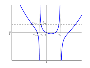
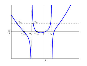
(a) $\bar{u}<0$	(b) $\bar{u}>0$

Figure 1. Illustration of the Laplace exponent and its roots when the drift $\overline{u}$ is negative and positive.

Due to the memoryless property of its jump-size distribution, the violation risk and regret can be obtained explicitly. The following two lemmas are due to Kou and Wang [20], Theorem 3.1 and its corollary. Here we let

$$l_{1,q}:=\frac{\eta_{-}-\xi_{1,q}}{\xi_{2,q}-\xi_{1,q}}>0\quad\textrm{and}\quad l_{2,q}:=\frac{\xi_{2,q}-\eta_{-}}{\xi_{2,q}-\xi_{1,q}}>0,\quad q\geq 0,$$

where, in particular, when $q=0$ and $\overline{u}<0$,

$$l_{1,0}=\frac{\eta_{-}}{\xi_{2,0}}>0\quad\textrm{and}\quad l_{2,0}=\frac{\xi_{2,0}-\eta_{-}}{\xi_{2,0}}>0.$$

Notice that $l_{1,q}+l_{2,q}=1$ for every $q\geq 0$.

Lemma 3.1 (violation risk).

For every $q\geq 0$ and $0<A<x$, we have

$$R_{x}^{(q)}(\tau_{A})=\frac{e^{-\eta_{-}A}}{\eta_{-}}\left[(\xi_{2,q}-\eta_{-})l_{1,q}e^{-\xi_{1,q}(x-A)}-(\eta_{-}-\xi_{1,q})l_{2,q}e^{-\xi_{2,q}(x-A)}\right].$$

In particular, when $q=0$ and $\overline{u}<0$, this reduces to

$$R_{x}^{(0)}(\tau_{A})=l_{2,0}e^{-\eta_{-}A}\left[1-e^{-\xi_{2,0}(x-A)}\right].$$

Lemma 3.2 (functional associated with the regret when $h\equiv 1$).

For every $q>0$, we have

$$\mathbb{E}^{x}\left[\int_{0}^{\tau_{A}}e^{-qt}{\rm d}t\right]=\frac{1}{q\eta_{-}}\left[l_{1,q}\xi_{2,q}\left(1-e^{-\xi_{1,q}(x-A)}\right)+l_{2,q}\xi_{1,q}\left(1-e^{-\xi_{2,q}(x-A)}\right)\right],\quad 0\leq A<x.$$

Furthermore, it can be extended to the case $q=0$, by taking $q\downarrow 0$ via (3.7) and the monotone convergence theorem;

$$\mathbb{E}^{x}\left[\tau_{A}\right]=\left\{\begin{array}[]{ll}\frac{1}{|\overline{u}|}\left[(x-A)+\frac{\xi_{2,0}-\eta_{-}}{\eta_{-}\xi_{2,0}}(1-e^{-\xi_{2,0}(x-A)})\right],&\textrm{if }\;\overline{u}<0,\\ \infty,&\textrm{if }\;\overline{u}\geq 0.\end{array}\right.$$

For a general Lévy process, Lemma 3.2 can be alternatively achieved by obtaining $\mathbb{P}^{x}\left\{\underline{X}_{\textbf{e}_{q}}<A\right\}$ where $\textbf{e}_{q}$ is an independent exponential random variable with parameter $q\geq 0$ and $\underline{X}_{t}:=\inf_{0\leq u\leq t}X_{u}$ is the running infimum of $X$; see Bertoin [5], Kyprianou [22] or Chapter 2 of Surya [39]. In particular, $\mathbb{P}^{x}\left\{\underline{X}_{\textbf{e}_{q}}<A\right\}$ admits an analytical form when jumps are of phase-type (Asmussen et al. [1]); the above results can be seen as its special case.

Remark 3.1.

As in Kou and Wang [20], we assume throughout this section that $X$ contains a diffusion component $(\sigma>0)$. Here we do not consider the case $\sigma=0$ because its spectrally negative case is covered in the next section. The results for $\sigma=0$ can be obtained similarly using the results by Asmussen et al. [1].

3.2. Optimal strategy when $h\equiv 1$

We shall obtain the optimal solution for $q\geq 0$. When $q=0$, we focus on the case when $\overline{u}<0$ because $\mathbb{E}^{x}\theta=\infty$ otherwise by Lemma 3.2 and the problem becomes trivial as we discussed in Section 2.

Suppose $q>0$. By Lemma 3.2, the stopping value (2.3) becomes

(3.8) $$G(x)=\gamma\mathbb{E}^{x}\left[\int_{0}^{\theta}e^{-qt}{\rm d}t\right]=\sum_{i=1,2}C_{i,q}\left(1-e^{-\xi_{i,q}x}\right)=\frac{\gamma}{q}-\sum_{i=1,2}C_{i,q}e^{-\xi_{i,q}x},\quad x>0,$$

where

(3.9) $$C_{1,q}:=\frac{\gamma}{q}\frac{l_{1,q}\xi_{2,q}}{\eta_{-}}\quad\textrm{and}\quad C_{2,q}:=\frac{\gamma}{q}\frac{l_{2,q}\xi_{1,q}}{\eta_{-}},$$

which satisfy

(3.10) $$\sum_{i=1,2}C_{i,q}=\frac{\gamma}{q}\quad\textrm{and}\quad\sum_{i=1,2}{C_{i,q}}\frac{\eta_{-}}{\eta_{-}-\xi_{i,q}}=\frac{\gamma}{q}.$$

The difference between the continuation and stopping values (defined in (2.5)) becomes, by Lemmas 3.1-3.2,

(3.11) $$\delta_{A}(x)=\frac{l_{1,q}}{\eta_{-}}\left[(\xi_{2,q}-\eta_{-})e^{-\xi_{1,q}(x-A)-\eta_{-}A}-\frac{\gamma}{q}\xi_{2,q}\left(1-e^{-\xi_{1,q}(x-A)}\right)\right]\\ +\frac{l_{2,q}}{\eta_{-}}\left[-(\eta_{-}-\xi_{1,q})e^{-\xi_{2,q}(x-A)-\eta_{-}A}-\frac{\gamma}{q}\xi_{1,q}\left(1-e^{-\xi_{2,q}(x-A)}\right)\right],\quad 0<A<x.$$

Suppose $q=0$ and $\overline{u}<0$. By Lemma 3.2, we have

$$G(x) =\frac{\gamma}{|\overline{u}|}\left[x+\frac{\xi_{2,0}-\eta_{-}}{\eta_{-}\xi_{2,0}}\left(1-e^{-\xi_{2,0}x}\right)\right],\quad x>0,$$

and taking $q\rightarrow 0$ in (3.11) via the monotone convergence theorem (or by Lemmas 3.1-3.2)

(3.12) $$\delta_{A}(x)=\frac{l_{1,0}}{\eta_{-}}\left[(\xi_{2,0}-\eta_{-})e^{-\eta_{-}A}-\frac{\gamma}{|\overline{u}|}\xi_{2,0}(x-A)\right]\\ +\frac{l_{2,0}}{\eta_{-}}\left[-\eta_{-}e^{-\xi_{2,0}(x-A)-\eta_{-}A}-\frac{\gamma}{|\overline{u}|}\left(1-e^{-\xi_{2,0}(x-A)}\right)\right],\quad 0<A<x.$$

Remark 3.2.

We have $\delta_{A}(A+)=0$ for every $A>0$, i.e., continuous fit holds whatever the choice of $A$ is. This is due to the fact that $X$ has paths of unbounded variation ($\sigma>0$). As we see in the next section, continuous fit is applied to identify the optimal threshold level for the bounded variation case. ∎

We shall obtain the threshold level $A^{*}$ such that the smooth fit condition holds, i.e., $\delta^{\prime}_{A^{*}}(A^{*}+)=0$ if such a threshold exists. By (3.11)-(3.12), we have

$$\delta_{A}^{\prime}(A+)=\left\{\begin{array}[]{ll}\frac{1}{\eta_{-}}\left[(\eta_{-}-\xi_{1,q})(\xi_{2,q}-\eta_{-})e^{-\eta_{-}A}-\frac{\gamma}{q}\xi_{1,q}\xi_{2,q}\right],&q>0\\ (\xi_{2,0}-\eta_{-})e^{-\eta_{-}A}-\frac{\gamma}{|\overline{u}|\eta_{-}}\xi_{2,0},&q=0\;\textrm{and}\;\overline{u}<0\end{array}\right\},\quad A>0.$$

Therefore, on condition that

(3.15) $$\left\{\begin{array}[]{ll}(\eta_{-}-\xi_{1,q})(\xi_{2,q}-\eta_{-})>\frac{\gamma}{q}\xi_{1,q}\xi_{2,q},&q>0\\ (\xi_{2,0}-\eta_{-})>\frac{\gamma}{|\overline{u}|\eta_{-}}\xi_{2,0},&q=0\;\textrm{and}\;\overline{u}<0\end{array}\right\},$$

the smooth fit condition $\delta^{\prime}_{A}(A+)=0$ is satisfied if and only if $A=A^{*}>0$ where

(3.18) $$A^{*}:=\left\{\begin{array}[]{ll}-\frac{1}{\eta_{-}}\log\left(\frac{\gamma}{q}\frac{\xi_{1,q}\xi_{2,q}}{(\eta_{-}-\xi_{1,q})(\xi_{2,q}-\eta_{-})}\right),&q>0,\\ -\frac{1}{\eta_{-}}\log\left(\frac{\gamma\xi_{2,0}}{|\overline{u}|\eta_{-}(\xi_{2,0}-\eta_{-})}\right),&q=0\;\textrm{ and }\;\overline{u}<0.\end{array}\right.$$

If (3.15) does not hold, we have $\delta_{A}^{\prime}(A+)<0$ for every $A>0$; in this case, we set $A^{*}=0$.

We now show that the optimal value function is $\phi:=\phi_{A^{*}}$ (see (2.9)). Suppose $q>0$ and $A^{*}>0$. Simple algebra shows that

(3.19) $$\delta(x):=\delta_{A^{*}}(x)=\frac{\gamma}{q}\frac{1}{\xi_{2,q}-\xi_{1,q}}\left[{\xi_{2,q}}\left(e^{-\xi_{1,q}(x-{A^{*}})}-1\right)-{\xi_{1,q}}\left(e^{-\xi_{2,q}(x-{A^{*}})}-1\right)\right],\quad x>A^{*}.$$

This together with (3.8) shows that

$$\phi(x)=\left\{\begin{array}[]{ll}\sum_{i=1,2}(L_{i,q}-C_{i,q})e^{-\xi_{i,q}x},&x>A^{*},\\ \frac{\gamma}{q}-\sum_{i=1,2}C_{i,q}e^{-\xi_{i,q}x},&0<x\leq A^{*},\\ 1,&x\leq 0,\end{array}\right.$$

where $C_{1,q}$ and $C_{2,q}$ are defined in (3.9) and

(3.20) $$L_{1,q}:=\frac{\gamma}{q}\frac{\xi_{2,q}}{\xi_{2,q}-\xi_{1,q}}e^{\xi_{1,q}{A^{*}}}\quad\textrm{and}\quad L_{2,q}:=-\frac{\gamma}{q}\frac{\xi_{1,q}}{\xi_{2,q}-\xi_{1,q}}e^{\xi_{2,q}{A^{*}}}.$$

When $q=0$ and $A^{*}>0$, we have

$$\delta(x) =-\frac{\gamma}{|\overline{u}|}\left[(x-A^{*})-\frac{1-e^{-\xi_{2,0}(x-A^{*})}}{\xi_{2,0}}\right],\quad x>A^{*},$$

and consequently,

$$\phi(x) =\left\{\begin{array}[]{ll}\frac{\gamma}{|\overline{u}|}\left(A^{*}+\frac{\xi_{2,0}-\eta_{-}}{\eta_{-}\xi_{2,0}}\left(1-e^{-\xi_{2,0}x}\right)+\frac{1}{\xi_{2,0}}(1-e^{-\xi_{2,0}(x-A^{*})})\right),&x>A^{*},\\ \frac{\gamma}{|\overline{u}|}\left(x+\frac{\xi_{2,0}-\eta_{-}}{\eta_{-}\xi_{2,0}}\left(1-e^{-\xi_{2,0}x}\right)\right),&0<x\leq A^{*},\\ 1,&x\leq 0.\end{array}\right.$$

Finally, it is understood for the case $A^{*}=0$ (for both $q>0$ and $q=0$) that

(3.21) $$\phi(x)=\lim_{\varepsilon\downarrow 0}\phi_{\varepsilon}(x)$$

where, by Lemma 3.1,

$$\lim_{\varepsilon\downarrow 0}R_{x}^{(q)}(\tau_{\varepsilon})=\mathbb{E}^{x}\left[e^{-q\theta}1_{\{X_{\theta}<0,\,\theta<\infty\}}\right]=\frac{(\eta_{-}-\xi_{1,q})(\xi_{2,q}-\eta_{-})}{\eta_{-}(\xi_{2,q}-\xi_{1,q})}\left(e^{-\xi_{1,q}x}-e^{-\xi_{2,q}x}\right).$$

This is the expectation of the cost incurred only when it jumps over the level zero.

When $A^{*}>0$ the value function $\phi$ can be attained by $\tau_{A^{*}}$, and when $A^{*}=0$ it can be approximated arbitrarily closely by $\phi_{\varepsilon}(x)$ (which is attained by $\tau_{\varepsilon}$) for sufficiently small $\varepsilon>0$. We therefore only need to verify that $\phi(x)\leq\mathbb{E}^{x}\left[e^{-q\tau}G(X_{\tau})1_{\{\tau<\infty\}}\right]$ for any $\tau\in\mathcal{S}$.

We first show that $\phi(\cdot)$ is dominated from above by the stopping value $G(\cdot)$.

Lemma 3.3.

We have $\phi(x)\leq G(x)$ for every $x\in\mathbb{R}$.

Proof.

For every $0<A<x$, ${\partial}\phi_{A}(x)/\partial A={\partial}\delta_{A}(x)/\partial A$ equals

$$\left\{\begin{array}[]{ll}\frac{1}{\eta_{-}}\left[l_{1,q}e^{-\xi_{1,q}(x-A)}+{l_{2,q}}e^{-\xi_{2,q}(x-A)}\right]\left[-(\eta_{-}-\xi_{1,q})(\xi_{2,q}-\eta_{-})e^{-\eta_{-}A}+{\frac{\gamma}{q}}\xi_{1,q}\xi_{2,q}\right],&q>0\\ \frac{1}{\eta_{-}}\left[l_{1,0}+l_{2,0}e^{-\xi_{2,0}(x-A)}\right]\left[-\eta_{-}(\xi_{2,0}-\eta_{-})e^{-\eta_{-}A}+\frac{\gamma}{|\overline{u}|}\xi_{2,0}\right],&q=0\;\textrm{and}\;\overline{u}<0\end{array}\right\}.$$

Here, in both cases, the term in the first bracket is strictly positive while that in the second bracket is increasing in $A$. Therefore, when $A^{*}>0$, $A^{*}$ is the unique value that makes it vanish, and consequently ${\partial}\phi_{A}(x)/\partial A\geq 0$ if and only if $A\geq A^{*}$. On the other hand, if $A^{*}=0$, ${\partial}\phi_{A}(x)/\partial A\geq 0$ for every $0<A<x$. These imply when $x>A^{*}$ that by Remark 3.2

$$\phi(x)\leq\lim_{A\uparrow x}\phi_{A}(x)=G(x)\quad\textrm{and}\quad\phi(x)=\lim_{\varepsilon\downarrow 0}\phi_{\varepsilon}(x)\leq\lim_{A\uparrow x}\phi_{A}(x)=G(x)$$

when $A^{*}>0$ and when $A^{*}=0$, respectively. On the other hand, when $-\infty<x\leq A^{*}$, we have $\phi(x)=G(x)$ by definition and hence the proof is complete. ∎

Remark 3.3.

1. Suppose $q>0$. In view of (3.8), $G(\cdot)$ is bounded from above by $\gamma/q$ uniformly on $x\in(0,\infty)$.

2. Suppose $\overline{u}<0$ and fix $x>0$. We have $G(x)\leq\mathbb{E}^{x}\theta<\infty$ uniformly on $q\geq 0$; namely, $G(x)$ is bounded by $\mathbb{E}^{x}\theta<\infty$ uniformly on $q\in[0,\infty)$.

3. Suppose $A^{*}>0$. Using the same argument as in the proof of Lemma 3.3, we have $\phi(x)\leq\lim_{\varepsilon\downarrow 0}\phi_{\varepsilon}(x)=\mathbb{E}^{x}\left[e^{-q\theta}1_{\{X_{\theta}<0,\,\theta<\infty\}}\right]\leq 1$ for every $x>A^{*}$. When $0<x\leq A^{*}$, using the monotonicity of $G(\cdot)$ and continuous fit (see Remark 3.2), we have $\phi(x)=G(x)\leq G(A^{*})=\phi(A^{*})\leq\lim_{\varepsilon\downarrow 0}\phi_{\varepsilon}(A^{*})\leq 1$. When $A^{*}=0$, we have $\phi(x)\leq 1$ in view of (3.21). Therefore, $\phi(\cdot)$ is uniformly bounded and it only takes values on $[0,1]$. ∎

Now we show that $\mathcal{L}\phi(x)\geq q\phi(x)$ on $(0,\infty)\backslash\{A^{*}\}$ where $\mathcal{L}$ is the infinitesimal generator of $X$ such that

(3.22) $$\mathcal{L}w(x)=\mu w^{\prime}(x)+\frac{1}{2}\sigma^{2}w^{\prime\prime}(x)+\lambda\int_{-\infty}^{\infty}\left[w(x+z)-w(x)\right]f(z){\rm d}z,\quad x\in\mathbb{R},$$

for any $C^{2}$-function $w:\mathbb{R}\rightarrow\mathbb{R}$. The proof for the following lemma is lengthy and technical, and therefore is relegated to the appendix.

Lemma 3.4.

1. If $A^{*}>0$, then we have

   (3.23) $$\mathcal{L}\phi(x)-q\phi(x) =0,\quad x>A^{*},$$

   (3.24) $$\mathcal{L}\phi(x)-q\phi(x) >0,\quad 0<x<A^{*}.$$

2. If $A^{*}=0$, then (3.23) holds for every $x>0$.

Lemmas 3.3 and 3.4 show the optimality. The proof is very similar to that of Proposition 4.1 given in the next section (see Appendix A.6) and hence we omit it.

Proposition 3.1.

We have

$$\phi(x)=\inf_{\tau\in\mathcal{S}}\mathbb{E}^{x}\left[e^{-q\tau}G(X_{\tau})1_{\left\{\tau<\infty\right\}}\right],\quad x>0.$$

4. Spectrally Negative Case

In this section, we analyze the case for a general spectrally negative Lévy process. We shall obtain the optimal strategy and the value function in terms of the scale function for a general $h$. We assume throughout this section that $q>0$. The results obtained here can in principle be extended to the case $q=0$ on condition that $\mathbb{E}^{x}\theta<\infty$ along the same line as in the discussion in the previous section. The proofs of all lemmas and propositions are given in the appendix.

4.1. Scale functions

Let $X$ be a spectrally negative Lévy process with its Laplace exponent

$$\psi(\beta):=\mathbb{E}^{0}\left[e^{\beta X_{1}}\right]=c\beta+\frac{1}{2}\sigma^{2}\beta^{2}+\int_{(0,\infty)}(e^{-\beta x}-1+\beta x1_{\{0<x<1\}})\,\Pi({\rm d}x),\quad{\beta\in\mathbb{R}},$$

where $c\in\mathbb{R}$, $\sigma\geq 0$ and $\Pi$ is a measure on $(0,\infty)$ such that $\int_{(0,\infty)}(1\wedge x^{2})\Pi({\rm d}x)<\infty$. See Kyprianou [22], p.212. In particular, when

(4.1) $$\int_{(0,\infty)}(1\wedge x)\,\Pi({\rm d}x)<\infty,$$

we can rewrite

$$\psi(\beta)=\mu\beta+\frac{1}{2}\sigma^{2}\beta^{2}+\int_{(0,\infty)}(e^{-\beta x}-1)\,\Pi({\rm d}x),\quad\beta\in\mathbb{R}$$

where

(4.2) $$\mu:=c+\int_{(0,1)}x\,\Pi({\rm d}x).$$

The process has paths of bounded variation if and only if $\sigma=0$ and (4.1) holds. It is also assumed that $X$ is not a negative subordinator (decreasing a.s.). Namely, we require $\mu$ to be strictly positive if $\sigma=0$.

It is well-known that $\psi$ is zero at the origin, convex on $\mathbb{R}_{+}$ and has a right-continuous inverse:

$$\zeta_{q}:=\sup\{\lambda\geq 0:\psi(\lambda)=q\},\quad q\geq 0.$$

Associated with every spectrally negative Lévy process, there exists a (q-)scale function

$$W^{(q)}:\mathbb{R}\rightarrow\mathbb{R};\quad q\geq 0,$$

that is continuous and strictly increasing on $[0,\infty)$ and satisfies

$$\int_{0}^{\infty}e^{-\beta x}W^{(q)}(x){\rm d}x=\frac{1}{\psi(\beta)-q},\qquad\beta>\zeta_{q}.$$

If $\tau_{a}^{+}$ is the first time the process goes above $a>x>0$, we have

$$\mathbb{E}^{x}\left[e^{-q\tau_{a}^{+}}1_{\left\{\tau_{a}^{+}<\theta,\,\tau_{a}^{+}<\infty\right\}}\right]=\frac{W^{(q)}(x)}{W^{(q)}(a)}\quad\textrm{and}\quad\mathbb{E}^{x}\left[e^{-q\theta}1_{\left\{\tau_{a}^{+}>\theta,\,\theta<\infty\right\}}\right]=Z^{(q)}(x)-Z^{(q)}(a)\frac{W^{(q)}(x)}{W^{(q)}(a)},$$

where

(4.3) $$Z^{(q)}(x):=1+q\int_{0}^{x}W^{(q)}(y){\rm d}y,\quad x\in\mathbb{R}.$$

Here we have

(4.4) $$W^{(q)}(x)=0\quad\text{on}\quad(-\infty,0)\quad\text{ and}\quad Z^{(q)}(x)=1\quad\text{on}\quad(-\infty,0].$$

We assume that $\Pi$ does not have atoms; this implies that $W^{(q)}$ is continuously differentiable on $(0,\infty)$. See Chan et al. [9] for the smoothness properties of the scale function.

The scale function increases exponentially; indeed, we have

(4.5) $$W^{(q)}(x)\sim\frac{e^{\zeta_{q}x}}{\psi^{\prime}(\zeta_{q})}\quad\textrm{as }\;x\rightarrow\infty.$$

There exists a (scaled) version of the scale function $W_{\zeta_{q}}=\{W_{\zeta_{q}}(x);x\in\mathbb{R}\}$ that satisfies, for every fixed $q\geq 0$,

$$W_{\zeta_{q}}(x)=e^{-\zeta_{q}x}W^{(q)}(x),\quad x\in\mathbb{R}$$

and

$$\int_{0}^{\infty}e^{-\beta x}W_{\zeta_{q}}(x){\rm d}x =\frac{1}{\psi(\beta+\zeta_{q})-q},\quad\beta>0.$$

Moreover $W_{\zeta_{q}}(x)$ is increasing and as is clear from (4.5)

(4.6) $$W_{\zeta_{q}}(x)\nearrow\frac{1}{\psi^{\prime}(\zeta_{q})}\quad\textrm{as }\;x\rightarrow\infty.$$

From Lemmas 4.3 and 4.4 of Kyprianou and Surya [24], we also have the following results about the behavior in the neighborhood of zero:

(4.12) $$W^{(q)}(0)=\left\{\begin{array}[]{ll}0,&\textrm{unbounded variation}\\ \frac{1}{\mu},&\textrm{bounded variation}\end{array}\right\}\quad\textrm{and}\quad W^{(q)^{\prime}}(0+)=\left\{\begin{array}[]{ll}\frac{2}{\sigma^{2}},&\sigma>0\\ \infty,&\sigma=0\;\textrm{and}\;\Pi(0,\infty)=\infty\\ \frac{q+\Pi(0,\infty)}{\mu^{2}},&\textrm{compound Poisson}\end{array}\right\}.$$

For a comprehensive account of the scale function, see Bertoin [5, 6], Kyprianou [22] and Kyprianou and Surya [24]. See Surya [40] and Egami and Yamazaki [13] for numerical methods for computing the scale function.

4.2. Rewriting the problem in terms of the scale function for a general $h$

We now rewrite the problem in terms of the scale function. For fixed $A\geq 0$, define a random measure

$$M^{(A,q)}(\omega,B):=\int_{0}^{\tau_{A}(\omega)}e^{-qt}1_{\left\{X_{t}(\omega)\in B\right\}}{\rm d}t,\quad\omega\in\Omega,\;B\in\mathcal{B}(\mathbb{R}).$$

Lemma 4.1.

For any $\omega\in\Omega$, we have

(4.13) $$\int_{0}^{\tau_{A}(\omega)}e^{-qt}h(X_{t}(\omega)){\rm d}t=\int_{\mathbb{R}}M^{(A,q)}(\omega,{\rm d}y)h(y).$$

With this lemma and the property of the random measure, we have

(4.14) $$\mathbb{E}^{x}\left[\int_{0}^{\tau_{A}}e^{-qt}h(X_{t}){\rm d}t\right]=\mathbb{E}^{x}\left[\int_{\mathbb{R}}M^{(A,q)}(\omega,{\rm d}y)h(y)\right]=\int_{\mathbb{R}}\mu_{x}^{(A,q)}({\rm d}y)h(y)$$

where

$$\mu_{x}^{(A,q)}(B):=\mathbb{E}^{x}\left[M^{(A,q)}(B)\right],\quad B\in\mathcal{B}(\mathbb{R})$$

is a version of the q-resolvent kernel that has a density owing to the Radon-Nikodym theorem; see Bertoin [6]. By using Theorem 1 of Bertoin [6] (see also Emery [15] and Suprun [38]), we have for every $B\in\mathcal{B}(\mathbb{R})$ and $a>x$

$$\mathbb{E}^{x}\left[\int_{0}^{\tau_{A}\wedge\tau^{+}_{a}}e^{-qt}1_{\left\{X_{t}\in B\right\}}{\rm d}t\right] =\int_{B\cap[A,\infty)}\Big{[}\frac{W^{(q)}(x-A)W^{(q)}(a-y)}{W^{(q)}(a-A)}-1_{\{x\geq y\}}W^{(q)}(x-y)\Big{]}{\rm d}y$$

$$=\int_{B\cap[A,\infty)}\Big{[}e^{-\zeta_{q}(y-A)}\frac{W^{(q)}(x-A)W_{\zeta_{q}}(a-y)}{W_{\zeta_{q}}(a-A)}-1_{\{x\geq y\}}W^{(q)}(x-y)\Big{]}{\rm d}y.$$

Moreover, by taking $a\uparrow\infty$ via the dominated convergence theorem in view of (4.6), we have

$$\mu_{x}^{(A,q)}(B) =\int_{B\cap[A,\infty)}\lim_{a\rightarrow\infty}\Big{[}e^{-\zeta_{q}(y-A)}\frac{W^{(q)}(x-A)W_{\zeta_{q}}(a-y)}{W_{\zeta_{q}}(a-A)}-1_{\{x\geq y\}}W^{(q)}(x-y)\Big{]}{\rm d}y$$

$$=\int_{B\cap[A,\infty)}\left[e^{-\zeta_{q}(y-A)}W^{(q)}(x-A)-1_{\{x\geq y\}}W^{(q)}(x-y)\right]{\rm d}y$$

where the second equality holds by (4.6). Hence, we have the following result.

Lemma 4.2.

Fix $q>0$ and $0<A<x$. We have

$$\mu_{x}^{(A,q)}({\rm d}y)=\left\{\begin{array}[]{ll}\Big{(}e^{-\zeta_{q}(y-A)}W^{(q)}(x-A)-1_{\{x\geq y\}}W^{(q)}(x-y)\Big{)}{\rm d}y,&y\geq A,\\ 0,&y<A.\end{array}\right.$$

By (4.14) and Lemma 4.2, we have, for any arbitrary $0<A<x$,

(4.15) $$\mathbb{E}^{x}\left[\int_{0}^{\tau_{A}}e^{-qt}h(X_{t}){\rm d}t\right]=W^{(q)}(x-A)\int_{0}^{\infty}e^{-\zeta_{q}y}h(y+A){\rm d}y-\int_{A}^{x}W^{(q)}(x-y)h(y){\rm d}y,$$

and this can be used to express the regret function and the stopping value. This also implies that the integrability condition (1.1) is equivalent to $\int_{0}^{\infty}e^{-\zeta_{q}y}h(y){\rm d}y<\infty$.

Using the $q$-resolvent kernel, we can also rewrite the violation risk.

Lemma 4.3.

For every $0<A<x$, we have

$$R^{(q)}_{x}(\tau_{A})=\frac{1}{\zeta_{q}}W^{(q)}(x-A)\int_{A}^{\infty}\Pi({\rm d}u)\left(1-e^{-\zeta_{q}(u-A)}\right)-\frac{1}{q}\int_{A}^{\infty}\Pi({\rm d}u)\left(Z^{(q)}(x-A)-Z^{(q)}(x-u)\right).$$

By (4.15) and Lemma 4.3, the difference function (2.5) becomes, for all $0<A<x$,

(4.16) $$\begin{split}\delta_{A}(x)&=R_{x}^{(q)}(\tau_{A})-\gamma\mathbb{E}^{x}\left[\int^{\tau_{A}}_{0}e^{-qt}h(X_{t}){\rm d}t\right]\\ &=\frac{1}{\zeta_{q}}W^{(q)}(x-A)\int_{A}^{\infty}\Pi({\rm d}u)\left(1-e^{-\zeta_{q}(u-A)}\right)-\frac{1}{q}\int_{A}^{\infty}\Pi({\rm d}u)\left(Z^{(q)}(x-A)-Z^{(q)}(x-u)\right)\\ &\qquad-\gamma\left[W^{(q)}(x-A)\int_{0}^{\infty}e^{-\zeta_{q}y}h(y+A){\rm d}y-\int_{A}^{x}W^{(q)}(x-y)h(y){\rm d}y\right].\end{split}$$

4.3. Continuous and smooth fit

We now apply continuous and smooth fit to obtain the candidate threshold levels for the bounded and unbounded variation cases, respectively. Firstly, the continuous fit condition $\delta_{A}(A+)=0$ requires in view of (4.16) that

(4.17) $$W^{(q)}(0)\Phi(A)=0$$

where

$$\Phi(A):=\frac{1}{\zeta_{q}}\int_{A}^{\infty}\Pi({\rm d}u)\left(1-e^{-\zeta_{q}(u-A)}\right)-\gamma\int_{0}^{\infty}e^{-\zeta_{q}y}h(y+A){\rm d}y,\quad A>0.$$

Note in this calculation we used the fact that the second term in (4.16) vanishes as $x\downarrow A$ by (4.4). The condition (4.17) automatically holds for the unbounded variation case by (4.12), but for the bounded variation case it requires

(4.18) $$\Phi(A)=0.$$

For the unbounded variation case, we apply smooth fit. For the violation risk, by using (4.3)-(4.4), we have

$$\left.\frac{\partial}{\partial x}R^{(q)}_{x}(\tau_{A})\right|_{x=A+} =\frac{1}{\zeta_{q}}W^{(q)^{\prime}}(0+)\int_{A}^{\infty}\Pi({\rm d}u)\left(1-e^{-\zeta_{q}(u-A)}\right).$$

For the regret function, by using (4.12) in particular $W^{(q)}(0)=0$, we obtain

$$\left.\frac{\partial}{\partial x}\mathbb{E}^{x}\left[\int_{0}^{\tau_{A}}e^{-qt}h(X_{t}){\rm d}t\right]\right|_{x=A+} =\lim_{x\downarrow A}\left[W^{(q)^{\prime}}(x-A)\int_{0}^{\infty}e^{-\zeta_{q}y}h(y+A){\rm d}y-\int_{A}^{x}W^{(q)^{\prime}}(x-y)h(y){\rm d}y\right]$$

$$=W^{(q)^{\prime}}(0+)\int_{0}^{\infty}e^{-\zeta_{q}y}h(y+A){\rm d}y.$$

Therefore, for the unbounded variation case, smooth fit requires

$$W^{(q)^{\prime}}(0+)\Phi(A)=0.$$

Consequently, once we get (4.18), continuous fit holds for the bounded variation case and both continuous and smooth fit holds for the unbounded variation case (see Figure 4 in Section 5 for an illustration). Because $h$ is non-decreasing by assumption, we have

$$\Phi^{\prime}(A)=-\int_{A}^{\infty}\Pi({\rm d}u)e^{-\zeta_{q}(u-A)}-\gamma\int_{0}^{\infty}e^{-\zeta_{q}y}h^{\prime}(y+A){\rm d}y<0,\quad A>0.$$

Hence there exists at most one root that satisfies (4.18). We let $A^{*}$ be the root if it exists and zero otherwise. Because $\lim_{A\uparrow\infty}\Phi(A)<0$, $A^{*}=0$ means that $\Phi(A)<0$ for all $A>0$.

4.4. Verification of optimality

We now show as in the last section that the optimal value function is $\phi:=\phi_{A^{*}}$ (see (2.9)) where in particular the case $A^{*}=0$ is defined by (3.21). When $A^{*}>0$, it can be attained by the strategy $\tau_{A^{*}}$ while when $A^{*}=0$ it can be approximated arbitrarily closely by $\tau_{\varepsilon}$ with sufficiently small $\varepsilon>0$. Recall that $\phi(x)=\delta(x)+G(x)$ (with $\delta:=\delta_{A^{*}}$) for $x>A^{*}$ and that $G(x)$ in (2.3) for $x>0$ can be expressed in terms of the scale function by taking the limit $A\downarrow 0$ in (4.15). The corresponding candidate value function becomes both for $A^{*}=0$ and for $A^{*}>0$

(4.19) $$\begin{split}\phi(x)&=\frac{1}{\zeta_{q}}W^{(q)}(x-A^{*})\int_{A^{*}}^{\infty}\Pi({\rm d}u)\left(1-e^{-\zeta_{q}(u-A^{*})}\right)-\frac{1}{q}\int_{A^{*}}^{\infty}\Pi({\rm d}u)\left(Z^{(q)}(x-A^{*})-Z^{(q)}(x-u)\right)\\ &+\gamma\left[W^{(q)}(x)\int_{0}^{\infty}e^{-\zeta_{q}y}h(y){\rm d}y-W^{(q)}(x-A^{*})\int_{0}^{\infty}e^{-\zeta_{q}y}h(y+A^{*}){\rm d}y-\int_{0}^{A^{*}}W^{(q)}(x-y)h(y){\rm d}y\right]\end{split}$$

for every $x>0$. By definition, $\phi(x)=1$ for every $x\leq 0$. In particular, when $A^{*}>0$, we can simplify by using (4.18),

$$\phi(x)=-\frac{1}{q}\int_{A^{*}}^{\infty}\Pi({\rm d}u)\left(Z^{(q)}(x-A^{*})-Z^{(q)}(x-u)\right)\\ +\gamma\left[W^{(q)}(x)\int_{0}^{\infty}e^{-\zeta_{q}y}h(y){\rm d}y-\int_{0}^{A^{*}}W^{(q)}(x-y)h(y){\rm d}y\right],\quad x>0.$$

These expressions for the candidate value function $\phi$ are valid not only on $(A^{*},\infty)$ but also on $(0,A^{*}]$ thanks to (4.4) and continuous fit.

In order to verify that $\phi$ is indeed optimal, we only need to show that (1) $\phi$ is dominated by $G$ and (2) $\mathcal{L}\phi(x)\geq q\phi(x)$ on $(0,\infty)\backslash\{A^{*}\}$ where

$$\mathcal{L}f(x) =cf^{\prime}(x)+\frac{1}{2}\sigma^{2}f^{\prime\prime}(x)+\int_{0}^{\infty}\left[f(x-z)-f(x)+f^{\prime}(x)z1_{\{0<z<1\}}\right]\Pi({\rm d}z),$$

$$\mathcal{L}f(x) =\mu f^{\prime}(x)+\int_{0}^{\infty}\left[f(x-z)-f(x)\right]\Pi({\rm d}z),$$

for the unbounded and bounded variation cases, respectively; see (4.2) for the definition of $\mu$. The former is proved in the following lemma:

Lemma 4.4.

We have $\phi(x)\leq G(x)$ for every $x\in\mathbb{R}$.

Now we recall that the processes $\left\{e^{-q(t\wedge\theta\wedge\tau_{a}^{+})}W^{(q)}(X_{t\wedge\theta\wedge\tau_{a}^{+}});t\geq 0\right\}$ and $\left\{e^{-q(t\wedge\theta\wedge\tau_{a}^{+})}Z^{(q)}(X_{t\wedge\theta\wedge\tau_{a}^{+}});t\geq 0\right\}$ are $\mathbb{P}^{x}$-martingales for any $0<x<a$; see page 229 in Kyprianou [22]. Therefore, we have

(4.20) $$\mathcal{L}W^{(q)}(x)=qW^{(q)}(x)\quad\textrm{and}\quad\mathcal{L}Z^{(q)}(x)=qZ^{(q)}(x),\quad x>0.$$

We take advantage of (4.20) to show the following lemma.

Lemma 4.5.

1. We have

   $$\mathcal{L}\phi(x)-q\phi(x)=0,\quad x>A^{*}.$$

2. If $A^{*}>0$, we have

   $$\mathcal{L}\phi(x)-q\phi(x)>0,\quad 0<x<A^{*}.$$

Finally, Lemmas 4.4-4.5 are used to show the optimality of $\phi$.

Proposition 4.1.

We have

$$\phi(x)=\inf_{\tau\in\mathcal{S}}\mathbb{E}^{x}\left[e^{-q\tau}G(X_{\tau})1_{\left\{\tau<\infty\right\}}\right],\quad x>0.$$

5. Numerical Results

We conclude this paper by providing numerical results on the models studied in Sections 3-4. We obtain optimal threshold levels $A^{*}$ for (1) the double exponential jump diffusion case with $h\equiv 1$, and for (2) the spectrally negative case with $h$ in the form of the exponential utility function. We study how the solution depends on the process $X$. We then verify continuous and smooth fit conditions for the bounded and unbounded variation cases, respectively.

5.1. The double exponential jump diffusion case with $h\equiv 1$

We evaluate the results obtained in Section 3 focusing on the case $h\equiv 1$. Here we plot the optimal threshold level $A^{*}$ defined in (3.18) as a function of $\gamma$. The values of $\xi_{1,q}$ and $\xi_{2,q}$ are obtained via the bisection method with error bound $10^{-4}$.

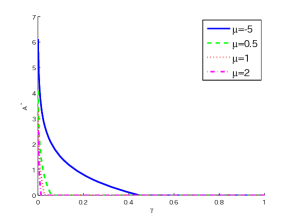
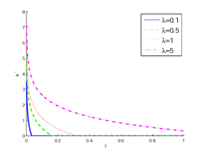
(i) $\mu$	(ii) $\lambda$
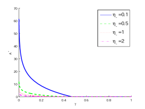
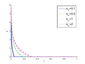
(iii) $\eta_{-}$	(iv) $\eta_{+}$
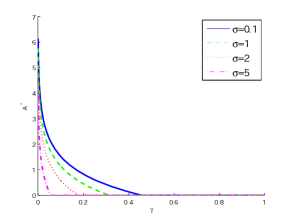
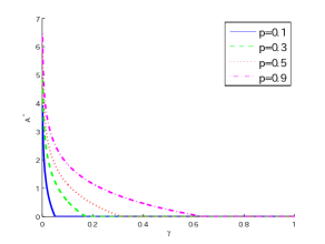
(v) $\sigma$	(vi) $p$

Figure 2. The optimal threshold level $A^{*}$ with respect to various parameters: the parameters are $\mu=-1$, $\sigma=1$, $\eta_{-}=1.0$, $\eta_{+}=2.0$, $p=0.5$, $\lambda=1$ unless they are specified.

Figure 2 shows how the optimal threshold level changes with respect to each parameter when $q=0.05$. The results obtained in (i)-(iv) and (vi) are consistent with our intuition because these parameters determine the overall drift $\overline{u}$, and $A^{*}$ is expected to decrease in $\overline{u}$. We show in (v) how it changes with respect to the diffusion coefficient $\sigma$; although it does not play a part in determining $\overline{u}$, we see that $A^{*}$ is in fact decreasing in $\sigma$. This is related to the fact that, as $\sigma$ increases, the probability of jumping over the level zero decreases.

5.2. The spectrally negative Lévy case with a general $h$

We now consider the spectrally negative case and verify the results obtained in Section 4. For the function $h$, we use the exponential utility function

$$h(x)=1-e^{-\rho x},\quad x>0.$$

Here $\rho>0$ is called the coefficient of absolute risk aversion. It is well-known that $\rho=-h^{\prime\prime}(x)/h(x)$ for every $x>0$, and, in particular, $h\equiv 1$ when $\rho=\infty$. We consider the tempered stable (CGMY) process and the variance gamma process with only downward jumps. The former has a Laplace exponent

$$\psi(\beta)=c\beta+C\lambda^{\alpha}\Gamma(-\alpha)\left\{\left(1+\frac{\beta}{\lambda}\right)^{\alpha}-1-\frac{\beta\alpha}{\lambda}\right\}$$

and a Lévy density given by

$$\Pi({\rm d}x)=C\frac{e^{-\lambda x}}{x^{1+\alpha}}1_{\{x>0\}}{\rm d}x$$

for some $\lambda>0$ and $\alpha<2$; see Surya [39] for the calculations. It has paths of bounded variation if and only if $\alpha<1$. When $\alpha=0$, it reduces to the variance gamma process; see Proposition 5.7.1 of Surya [39] for the form of its Laplace exponent. We consider the case when $\sigma=0$. The optimal threshold levels are computed by the bisection method using (4.18) with error bound $10^{-6}$.

Figure 3 shows the optimal threshold level $A^{*}$ as a function of $\gamma$ with various values of $\rho$. We see that it is indeed monotonically decreasing in $\rho$. This can be also analytically verified in view of the definition of $\Phi(A)$ because $h$ is decreasing in $\rho$ for every fixed $A$, and consequently the root $A^{*}$ must be decreasing in $\rho$. This is also clear because the regret function monotonically decreases in $\rho$.

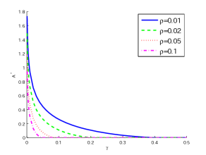
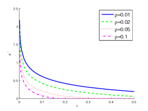
(a) tempered stable (unbounded variation)	(b) tempered stable (bounded variation)

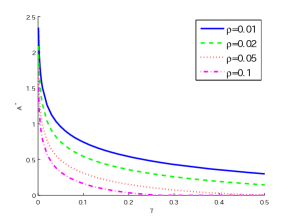
(c) variance gamma

Figure 3. The optimal threshold level $A^{*}$ with various values of coefficients of absolute risk aversion $\rho$: (a) tempered stable (unbounded variation) with $\alpha=1.5$, $\lambda=2$, $C=0.05$ and $c=0.05$, (b) tempered stable (bounded variation) with $\alpha=0.8$, $\lambda=2$, $C=0.075$ and $c=0.05$, and (c) variance gamma with with $\lambda=2$, $C=0.075$ and $c=0.05$.

5.3. Continuous and smooth fit

We conclude this section by numerically verifying the continuous and smooth fit conditions. Unlike the optimal threshold level $A^{*}$, the computation of the value function $\phi$ involves that of the scale function. Here we consider the spectrally negative Lévy process with exponential jumps in the form (3.1) with $p=1$ and $\sigma\geq 0$. We consider the bounded variation case ($\sigma=0$) and the unbounded variation case ($\sigma>0$). We also set $h\equiv 1$. This is a special case of the spectrally negative Lévy process with phase-type jumps, and its scale function can be obtained analytically as in Egami and Yamazaki [13]. In general, scale functions can be approximated by Laplace inversion algorithm by Surya [40] or the phase-type fitting approach by Egami and Yamazaki [13]. One drawback of the approximation methods of the scale function is that the error tends to explode as $x$ gets large (see (4.5)). Because our objective here is to accurately verify the continuous and smooth fit conditions, we use an example where an explicit form is known. Notice that the threshold level $A^{*}$ can be computed independently of the scale function, and hence one can alternatively approximate the value function $\phi$ by simulation.

Figure 4 draws the stopping value $G$ as well as the value function $\phi$ for both the bounded and unbounded variation cases. The value function $\phi$ is indeed continuous at $A^{*}$ for the bounded variation case and differentiable for the unbounded variation case. It can be seen that $G$ indeed dominates $\phi$. While $G$ is monotonically increasing on $(0,\infty)$, $\phi$ is decreasing for large $x$ and is expected to converge to zero as $x\rightarrow\infty$.

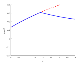
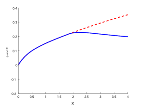
(a) continuous fit	(b) smooth fit

Figure 4. Illustration of $\phi$ (solid) and $G$ (dotted) for (a) the bounded variation case with $\sigma=0$ and $\mu=0.3$ and (b) the unbounded variation case with $\sigma=0.5$ and $\mu=0.175$. Other parameters are $q=0.05$, $h\equiv 1$, $\lambda=0.5$, $\eta_{-}=1$ and $\gamma=0.04$.

Appendix A Proofs

A.1. Proof of Lemma 3.4

We shall prove for the case $q>0$ and then extend it to the case $q=0$ and $\overline{u}<0$. We first prove the following for the proof of Lemma 3.4.

Lemma A.1.

Fix $q>0$ and $x\in\mathbb{R}$. Suppose that a function $w:\mathbb{R}\rightarrow\mathbb{R}$ in a neighborhood of $x>0$ is given by

$$w(x)=k+\sum_{i=1,2}k_{i}e^{-\xi_{i,q}x}$$

for some $k$, $k_{1}$ and $k_{2}$ in $\mathbb{R}$. Then we have

$$q(w(x)-k)=\mathcal{L}w(x)-\lambda\left[\int_{-\infty}^{\infty}w(x+z)f(z){\rm d}z-\left(k+\sum_{i=1,2}k_{i}\left(\frac{p\eta_{-}}{\eta_{-}-\xi_{i,q}}+\frac{(1-p)\eta_{+}}{\eta_{+}+\xi_{i,q}}\right)e^{-\xi_{i,q}x}\right)\right].$$

Proof.

Because $\psi(-\xi_{1,q})=\psi(-\xi_{2,q})=q$, we have

$$q(w(x)-k)=\sum_{i=1,2}k_{i}\psi(-\xi_{i,q})e^{-\xi_{i,q}x}.$$

Moreover, the right-hand side equals by (3.3)

$$\sum_{i=1,2}k_{i}\left[-\mu\xi_{i,q}+\frac{1}{2}\sigma^{2}(\xi_{i,q})^{2}+\lambda\left(\frac{p\eta_{-}}{\eta_{-}-\xi_{i,q}}+\frac{(1-p)\eta_{+}}{\eta_{+}+\xi_{i,q}}-1\right)\right]e^{-\xi_{i,q}x}$$

$$=-\lambda(w(x)-k)+\sum_{i=1,2}k_{i}\left[-\mu\xi_{i,q}+\frac{1}{2}\sigma^{2}(\xi_{i,q})^{2}+\lambda\left(\frac{p\eta_{-}}{\eta_{-}-\xi_{i,q}}+\frac{(1-p)\eta_{+}}{\eta_{+}+\xi_{i,q}}\right)\right]e^{-\xi_{i,q}x}$$

$$=\frac{1}{2}\sigma^{2}w^{\prime\prime}(x)+\mu w^{\prime}(x)-\lambda w(x)+\lambda k+\lambda\sum_{i=1,2}k_{i}\left(\frac{p\eta_{-}}{\eta_{-}-\xi_{i,q}}+\frac{(1-p)\eta_{+}}{\eta_{+}+\xi_{i,q}}\right)e^{-\xi_{i,q}x}$$

$$=\mathcal{L}w(x)-\lambda\left[\int_{-\infty}^{\infty}w(x+z)f(z){\rm d}z-\left(k+\sum_{i=1,2}k_{i}\left(\frac{p\eta_{-}}{\eta_{-}-\xi_{i,q}}+\frac{(1-p)\eta_{+}}{\eta_{+}+\xi_{i,q}}\right)e^{-\xi_{i,q}x}\right)\right],$$

as desired. ∎

Proof of Lemma 3.4 when $q>0$.

(i) Suppose $A^{*}>0$. By Lemma A.1 above, we have $\mathcal{L}\phi(x)-q\phi(x)$ equals, for every $x>{A^{*}}$,

(A.1) $$\lambda\left[\int_{-\infty}^{\infty}\phi(x+z)f(z){\rm d}z-\sum_{i=1,2}(L_{i,q}-C_{i,q})\left(\frac{p\eta_{-}}{\eta_{-}-\xi_{i,q}}+\frac{(1-p)\eta_{+}}{\eta_{+}+\xi_{i,q}}\right)e^{-\xi_{i,q}x}\right],$$

and, for every $0<x<{A^{*}}$,

(A.2) $$-(q+\lambda)\frac{\gamma}{q}+\lambda\left[\int_{-\infty}^{\infty}\phi(x+z)f(z){\rm d}z+\sum_{i=1,2}C_{i,q}\left(\frac{p\eta_{-}}{\eta_{-}-\xi_{i,q}}+\frac{(1-p)\eta_{+}}{\eta_{+}+\xi_{i,q}}\right)e^{-\xi_{i,q}x}\right]$$

by using (3.8) and (3.20).

Proof of (3.23). We only need to show (A.1) equals zero. Notice that the integral can be split into four parts, and, by using (3.9)-(3.10), we have

$$\int_{0}^{\infty}\phi(x+z)f(z){\rm d}z =\sum_{i=1,2}(L_{i,q}-C_{i,q})\frac{(1-p)\eta_{+}}{\eta_{+}+\xi_{i,q}}e^{-\xi_{i,q}x},$$

$$\int_{-(x-{A^{*}})}^{0}\phi(x+z)f(z){\rm d}z =\sum_{i=1,2}(L_{i,q}-C_{i,q})\frac{p\eta_{-}}{\eta_{-}-\xi_{i,q}}e^{-\xi_{i,q}x}-\sum_{i=1,2}(L_{i,q}-C_{i,q})\frac{p\eta_{-}}{\eta_{-}-\xi_{i,q}}e^{-\eta_{-}(x-{A^{*}})-\xi_{i,q}{A^{*}}},$$

$$\int^{-(x-{A^{*}})}_{-x}\phi(x+z)f(z){\rm d}z =\frac{p\gamma}{q}e^{-\eta_{-}(x-{A^{*}})}-\sum_{i=1,2}C_{i,q}\frac{p\eta_{-}}{\eta_{-}-\xi_{i,q}}e^{-\eta_{-}(x-{A^{*}})-\xi_{i,q}{A^{*}}},$$

$$\int_{-\infty}^{-x}\phi(x+z)f(z){\rm d}z =pe^{-\eta_{-}x}.$$

Putting altogether, (A.1) equals

$$-\sum_{i=1,2}L_{i,q}\frac{p\eta_{-}}{\eta_{-}-\xi_{i,q}}e^{-\eta_{-}(x-{A^{*}})-\xi_{i,q}{A^{*}}}+{\frac{p\gamma}{q}}e^{-\eta_{-}(x-{A^{*}})}+pe^{-\eta_{-}x}\\ =pe^{-\eta_{-}x}\left[1-{\frac{\gamma}{q}}\frac{\xi_{1,q}\xi_{2,q}}{(\eta_{-}-\xi_{1,q})(\xi_{2,q}-\eta_{-})}e^{\eta_{-}{A^{*}}}\right],$$

and this vanishes because of the way $A^{*}$ is chosen in (3.18).

Proof of (3.24). We shall show that (A.2) is decreasing in $x$. Note that $\int_{-\infty}^{\infty}\phi(x+z)f(z){\rm d}z$ can be split into four parts with

$$\int_{{A^{*}}-x}^{\infty}\phi(x+z)f(z){\rm d}z =(1-p)\sum_{i=1,2}(L_{i,q}-C_{i,q})\frac{\eta_{+}}{\xi_{i,q}+\eta_{+}}e^{-\eta_{+}(A^{*}-x)-\xi_{i,q}{A^{*}}},$$

$$\int_{0}^{{A^{*}}-x}\phi(x+z)f(z){\rm d}z =(1-p)\left[\frac{\gamma}{q}\left(1-e^{-\eta_{+}({A^{*}}-x)}\right)-\sum_{i=1,2}C_{i,q}\frac{\eta_{+}}{\xi_{i,q}+\eta_{+}}\left(e^{-x\xi_{i,q}}-e^{-\eta_{+}(A^{*}-x)-\xi_{i,q}{A^{*}}}\right)\right],$$

$$\int_{-x}^{0}\phi(x+z)f(z){\rm d}z =\frac{p\gamma}{q}-p\sum_{i=1,2}C_{i,q}\frac{\eta_{-}}{\eta_{-}-\xi_{i,q}}e^{-\xi_{i,q}x},$$

$$\int_{-\infty}^{-x}\phi(x+z)f(z){\rm d}z =pe^{-\eta_{-}x},$$

and after some algebra, we have

$$\int_{-\infty}^{\infty}\phi(x+z)f(z){\rm d}z+\sum_{i=1,2}C_{i,q}\left(\frac{p\eta_{-}}{\eta_{-}-\xi_{i,q}}+\frac{(1-p)\eta_{+}}{\eta_{+}+\xi_{i,q}}\right)e^{-\xi_{i,q}x}\\ =\frac{\gamma}{q}+pe^{-\eta_{-}x}+(1-p)e^{\eta_{+}(x-{A^{*}})}\left(-\frac{\gamma}{q}+\sum_{i=1,2}L_{i,q}\frac{\eta_{+}}{\xi_{i,q}+\eta_{+}}e^{-\xi_{i,q}{A^{*}}}\right),$$

which by (3.20) equals to

$$\frac{\gamma}{q}+pe^{-\eta_{-}x}+(1-p)e^{-\eta_{+}({A^{*}}-x)}\frac{\gamma}{\xi_{2,q}-\xi_{1,q}}\frac{\xi_{1,q}\xi_{2,q}}{q}\left(\frac{1}{\xi_{2,q}+\eta_{+}}-\frac{1}{\xi_{1,q}+\eta_{+}}\right).$$

Hence we see that (A.2) or $\mathcal{L}\phi(x)-q\phi(x)$ equals

$$-\gamma+\lambda\left[pe^{-\eta_{-}x}-(1-p)e^{-\eta_{+}({A^{*}}-x)}\frac{\xi_{1,q}\xi_{2,q}}{q}\frac{\gamma}{(\xi_{2,q}+\eta_{+})(\xi_{1,q}+\eta_{+})}\right]$$

and is therefore decreasing in $x$ on $(0,A^{*})$. We now only need to show that $\lim_{x\uparrow A^{*}}\left(\mathcal{L}\phi(x)-q\phi(x)\right)>0$.

For every $x>A^{*}$,

$$\delta^{\prime\prime}(x)=\frac{\gamma}{q}\frac{\xi_{1,q}\xi_{2,q}}{\xi_{2,q}-\xi_{1,q}}\left[\xi_{1,q}e^{-\xi_{1,q}(x-{A^{*}})}-{\xi_{2,q}}e^{-\xi_{2,q}(x-{A^{*}})}\right],$$

and hence, after taking $x\downarrow A^{*}$,

$$\delta^{\prime\prime}({A^{*}+})=-\frac{\gamma}{q}\xi_{1,q}\xi_{2,q}<0.$$

Consequently, by the continuous and smooth fit conditions $\delta(A^{*}+)=\delta^{\prime}(A^{*}+)=0$ and the definition of $\mathcal{L}$ in (3.22), we have

$$\lim_{x\uparrow{A^{*}}}\left(\mathcal{L}\phi(x)-q\phi(x)\right)>\lim_{x\downarrow{A^{*}}}\left(\mathcal{L}\phi(x)-q\phi(x)\right)=0,$$

as desired.

(ii) Suppose $A^{*}=0$. By (3.21), we have

$$\phi(x)=C\left(e^{-\xi_{1,q}x}-e^{-\xi_{2,q}x}\right),\quad x>0$$

where

$$C:=\frac{(\eta_{-}-\xi_{1,q})(\xi_{2,q}-\eta_{-})}{\eta_{-}(\xi_{2,q}-\xi_{1,q})}.$$

By Lemma A.1 above, we have $\mathcal{L}\phi(x)-q\phi(x)$ equals, for every $x>0$,

$$\lambda\left[\int_{-\infty}^{\infty}\phi(x+z)f(z){\rm d}z-\sum_{i=1,2}C\left(\frac{p\eta_{-}}{\eta_{-}-\xi_{i,q}}+\frac{(1-p)\eta_{+}}{\eta_{+}+\xi_{i,q}}\right)e^{-\xi_{i,q}x}\right],$$

and this vanishes after some algebra. ∎

Proof of Lemma 3.4 when $q=0$.

We extend the results above to the case $q=0$ and $\overline{u}<0$. Solely in this proof, let us emphasize the dependence on $q$ and use $A^{*}_{q}$, $\phi_{q}(\cdot)$, $G_{q}(\cdot)$, $\delta_{q}(\cdot)$, and $\delta_{A,q}(\cdot)$ with a specified discount rate $q\geq 0$. We shall show that $\mathcal{L}\phi_{0}(x)=\lim_{q\rightarrow 0}\mathcal{L}\phi_{q}(x)$ for all $x>0$. First notice that $A^{*}_{q}\rightarrow A^{*}_{0}$ as $q\rightarrow 0$.

Clearly, $G_{q}(x)\rightarrow G_{0}(x)$ by the monotone convergence theorem. Furthermore, we have

$$G_{q}^{\prime}(x) =\frac{\gamma}{q\eta_{-}}\xi_{1,q}\xi_{2,q}\sum_{i=1,2}l_{i,q}e^{-\xi_{i,q}x}\xrightarrow{q\downarrow 0}\frac{\gamma}{|\overline{u}|}\left[1+\frac{\xi_{2,0}-\eta_{-}}{\eta_{-}}e^{-\xi_{2,0}x}\right]=G_{0}^{\prime}(x),$$

$$G_{q}^{\prime\prime}(x) =-\frac{\gamma}{q\eta_{-}}\xi_{1,q}\xi_{2,q}\sum_{i=1,2}\xi_{i,q}l_{i,q}e^{-\xi_{i,q}x}\xrightarrow{q\downarrow 0}-\frac{\gamma}{|\overline{u}|}\left[\frac{(\xi_{2,0}-\eta_{-})\xi_{2,0}}{\eta_{-}}e^{-\xi_{2,0}x}\right]=G_{0}^{\prime\prime}(x).$$

Fix $x>A_{0}^{*}$. We suppose $A_{0}^{*}=0$ and focus on $q\in[0,q_{0}]$ with $q_{0}>0$ sufficiently small such that $A_{q}^{*}=0$ for all $0\leq q\leq q_{0}$. We have, by applying the monotone convergence theorem on (3.21), $\phi_{q}(x)\rightarrow\phi_{0}(x)$ as $q\rightarrow 0$. Furthermore,

$$\phi^{\prime}_{q}(x)=\frac{(\eta_{-}-\xi_{1,q})(\xi_{2,q}-\eta_{-})}{\eta_{-}(\xi_{2,q}-\xi_{1,q})}\left(-\xi_{1,q}e^{-\xi_{1,q}x}+\xi_{2,q}e^{-\xi_{2,q}x}\right)\xrightarrow{q\downarrow 0}\xi_{2,0}e^{-\xi_{2,0}x}=\phi_{0}^{\prime}(x),$$

$$\phi_{q}^{\prime\prime}(x)=\frac{(\eta_{-}-\xi_{1,q})(\xi_{2,q}-\eta_{-})}{\eta_{-}(\xi_{2,q}-\xi_{1,q})}\left(\xi_{1,q}^{2}e^{-\xi_{1,q}x}-\xi_{2,q}^{2}e^{-\xi_{2,q}x}\right)\xrightarrow{q\downarrow 0}-\xi_{2,0}^{2}e^{-\xi_{2,0}x}=\phi_{0}^{\prime\prime}(x).$$

Suppose $A_{0}^{*}>0$ and focus on $q\in[0,q_{0}]$ with $q_{0}>0$ sufficiently small such that $x>A_{q}^{*}$ for all $0\leq q\leq q_{0}$. Note that

$$|\delta_{q}(x)-\delta_{0}(x)|\leq|\delta_{q}(x)-\delta_{A_{q}^{*},0}(x)|+|\delta_{A_{q}^{*},0}(x)-\delta_{0}(x)|$$

where on the right-hand side the former vanishes as $q\rightarrow 0$ by the monotone convergence theorem in view of (2.5) and the latter vanishes because $A_{q}^{*}\rightarrow A_{0}^{*}$; hence $\delta_{q}(x)\rightarrow\delta_{0}(x)$ as $q\rightarrow 0$. Furthermore,

$$\delta_{q}^{\prime}(x) =\frac{\gamma}{q}\frac{\xi_{1,q}\xi_{2,q}}{\xi_{2,q}-\xi_{1,q}}\left[-e^{-\xi_{1,q}(x-A^{*}_{q})}+e^{-\xi_{2,q}(x-A^{*}_{q})}\right]\xrightarrow{q\downarrow 0}-\frac{\gamma}{|\overline{u}|}\left[1-e^{-\xi_{2,0}(x-A^{*}_{0})}\right]=\delta_{0}^{\prime}(x),$$

$$\delta_{q}^{\prime\prime}(x) =\frac{\gamma}{q}\frac{\xi_{1,q}\xi_{2,q}}{\xi_{2,q}-\xi_{1,q}}\left[\xi_{1,q}e^{-\xi_{1,q}(x-A^{*}_{q})}-\xi_{2,q}e^{-\xi_{2,q}(x-A^{*}_{q})}\right]\xrightarrow{q\downarrow 0}-\frac{\gamma}{|\overline{u}|}\xi_{2,0}e^{-\xi_{2,0}(x-A^{*}_{0})}=\delta_{0}^{\prime\prime}(x).$$

In summary, we have $\phi_{q}(x)\rightarrow\phi_{0}(x)$, $\phi_{q}^{\prime}(x)\rightarrow\phi_{0}^{\prime}(x)$ and $\phi_{q}^{\prime\prime}(x)\rightarrow\phi_{0}^{\prime\prime}(x)$ as $q\rightarrow 0$ for every $x>0$. Moreover, by Remark 3.3-(3), via the dominated convergence theorem,

$$\int_{-\infty}^{\infty}\phi_{0}(x+z)f(z){\rm d}z=\lim_{q\rightarrow\infty}\int_{-\infty}^{\infty}\phi_{q}(x+z)f(z){\rm d}z,\quad x\geq 0.$$

Consequently, $\lim_{q\rightarrow 0}\left(\mathcal{L}\phi_{q}(x)-q\phi_{q}(x)\right)=\mathcal{L}\phi_{0}(x)$. This together with the result for $q>0$ shows the claim. ∎

A.2. Proof of Lemma 4.1

Because $h$ is continuous on $(0,\infty)$, it is Borel measurable. Hence there exists a converging sequence of simple functions $(h^{(n)})_{n\in\mathbb{N}}$ increasing to $h$ in the form

$$h^{(n)}(y):=\sum_{i=1}^{l(n)}b_{i}^{(n)}1_{\left\{y\in B_{n,i}\right\}},\quad n\geq 1,$$

for some $l:\mathbb{N}\rightarrow\mathbb{N}$, $\{b_{i}^{(n)};n\geq 1,0\leq i\leq l(n)\}$ and Borel measurable sets $\left\{B_{n,i};n\geq 1,0\leq i\leq l(n)\right\}$. See page 99 of Cinlar and Vanderbei [11].

Then the right-hand side of (4.13) is, by the monotone convergence theorem,

$$\int_{\mathbb{R}}M^{(A,q)}(\omega,{\rm d}y)h(y)=\int_{\mathbb{R}}M^{(A,q)}(\omega,{\rm d}y)\lim_{n\rightarrow\infty}\sum_{i=1}^{l(n)}b_{i}^{(n)}1_{\left\{y\in B_{n,i}\right\}}\\ =\lim_{n\rightarrow\infty}\sum_{i=1}^{l(n)}b_{i}^{(n)}\int_{\mathbb{R}}M^{(A,q)}(\omega,{\rm d}y)1_{\left\{y\in B_{n,i}\right\}}=\lim_{n\rightarrow\infty}\sum_{i=1}^{l(n)}b_{i}^{(n)}M^{(A,q)}(\omega,B_{n,i}).$$

This is indeed equal to the left-hand side of (4.13) because, by the monotone convergence theorem,

$$\int_{0}^{\tau_{A}(\omega)}e^{-qt}h(X_{t}(\omega)){\rm d}t=\int_{0}^{\tau_{A}(\omega)}e^{-qt}\lim_{n\rightarrow\infty}\sum_{i=1}^{l(n)}b_{i}^{(n)}1_{\left\{X_{t}(\omega)\in B_{n,i}\right\}}{\rm d}t\\ =\lim_{n\rightarrow\infty}\sum_{i=1}^{l(n)}b_{i}^{(n)}\int_{0}^{\tau_{A}(\omega)}e^{-qt}1_{\left\{X_{t}(\omega)\in B_{n,i}\right\}}{\rm d}t=\lim_{n\rightarrow\infty}\sum_{i=1}^{l(n)}b_{i}^{(n)}M^{(A,q)}(\omega,B_{n,i}),$$

as desired.

A.3. Proof of Lemma 4.3

Let $N(\cdot,\cdot)$ be the Poisson random measure for $-X$ and $\underline{X}_{t}:=\min_{0\leq s\leq t}X_{s}$ for all $t\geq 0$. By the compensation formula (see, e.g., Theorem 4.4 in Kyprianou [22]), we have

$$R^{(q)}_{x}(\tau_{A}) =\mathbb{E}^{x}\left[\int_{0}^{\infty}\int_{0}^{\infty}N({\rm d}t,{\rm d}u)e^{-qt}1_{\{X_{t-}-u\leq 0,\,\underline{X}_{t-}>A\}}\right]$$

$$=\mathbb{E}^{x}\left[\int_{0}^{\infty}e^{-qt}{\rm d}t\int_{0}^{\infty}\Pi({\rm d}u)1_{\{X_{t-}-u\leq 0,\,\underline{X}_{t-}>A\}}\right]$$

$$=\int_{0}^{\infty}\Pi({\rm d}u)\int_{0}^{\infty}{\rm d}t\left[e^{-qt}\mathbb{P}^{x}\{X_{t-}\leq u,\underline{X}_{t-}>A\}\right]$$

$$=\int_{0}^{\infty}\Pi({\rm d}u)\int_{0}^{\infty}{\rm d}t\left[e^{-qt}\mathbb{P}^{x}\{X_{t-}\leq u,\tau_{A}\geq t\}\right].$$

By using the $q$-resolvent kernel that appeared in Lemma 4.2, we have for $u>A$

$$\int_{0}^{\infty}{\rm d}t\left[e^{-qt}\mathbb{P}^{x}\{X_{t-}\leq u,\tau_{A}\geq t\}\right] =\int_{A}^{u}{\rm d}y\left[e^{-\zeta_{q}(y-A)}W^{(q)}(x-A)-W^{(q)}(x-y)\right]$$

$$=\int_{0}^{u-A}{\rm d}z\left[e^{-\zeta_{q}z}W^{(q)}(x-A)-W^{(q)}(x-z-A)\right]$$

$$=\frac{1}{\zeta_{q}}W^{(q)}(x-A)\left(1-e^{-\zeta_{q}(u-A)}\right)-\int_{0}^{u-A}{\rm d}zW^{(q)}(x-z-A),$$

and it is zero on $0\leq u\leq A$. Substituting this, we have

$$R^{(q)}_{x}(\tau_{A})=\int_{A}^{\infty}\Pi({\rm d}u)\left\{\frac{1}{\zeta_{q}}W^{(q)}(x-A)\left(1-e^{-\zeta_{q}(u-A)}\right)-\int_{0}^{u-A}{\rm d}zW^{(q)}(x-A-z)\right\}.$$

By (4.4), we have

$$R^{(q)}_{x}(\tau_{A}) =\frac{1}{\zeta_{q}}W^{(q)}(x-A)\int_{A}^{\infty}\Pi({\rm d}u)\left(1-e^{-\zeta_{q}(u-A)}\right)$$

$$\qquad-\int_{A}^{x}\Pi({\rm d}u)\int_{0}^{u-A}{\rm d}zW^{(q)}(x-A-z)-\int_{x}^{\infty}\Pi({\rm d}u)\int_{0}^{x-A}{\rm d}zW^{(q)}(x-A-z)$$

$$=\frac{1}{\zeta_{q}}W^{(q)}(x-A)\int_{A}^{\infty}\Pi({\rm d}u)\left(1-e^{-\zeta_{q}(u-A)}\right)$$

$$\qquad-\frac{1}{q}\int_{A}^{x}\Pi({\rm d}u)\left(Z^{(q)}(x-A)-Z^{(q)}(x-u)\right)-\frac{1}{q}\int_{x}^{\infty}\Pi({\rm d}u)\left(Z^{(q)}(x-A)-1\right)$$

$$=\frac{1}{\zeta_{q}}W^{(q)}(x-A)\int_{A}^{\infty}\Pi({\rm d}u)\left(1-e^{-\zeta_{q}(u-A)}\right)-\frac{1}{q}\int_{A}^{\infty}\Pi({\rm d}u)\left(Z^{(q)}(x-A)-Z^{(q)}(x-u)\right),$$

as desired.

A.4. Proof of Lemma 4.4

Fix $0<A<x$. We have

$$\frac{\partial}{\partial A}R_{x}^{(q)}(\tau_{A}) =\left(W^{(q)}(x-A)-\frac{1}{\zeta_{q}}W^{(q)^{\prime}}(x-A)\right)\int_{A}^{\infty}\Pi({\rm d}u)\left(1-e^{-\zeta_{q}(u-A)}\right)$$

$$=-\frac{1}{\zeta_{q}}W_{\zeta_{q}}^{\prime}(x-A)e^{\zeta_{q}(x-A)}\int_{A}^{\infty}\Pi({\rm d}u)\left(1-e^{-\zeta_{q}(u-A)}\right),$$

and because we can write

$$\mathbb{E}^{x}\left[\int_{0}^{\tau_{A}}e^{-qt}h(X_{t}){\rm d}t\right]=e^{\zeta_{q}x}W_{\zeta_{q}}(x-A)\int_{A}^{\infty}e^{-\zeta_{q}y}h(y){\rm d}y-\int_{A}^{x}W^{(q)}(x-y)h(y){\rm d}y,$$

we have

$$\frac{\partial}{\partial A}\mathbb{E}^{x}\left[\int_{0}^{\tau_{A}}e^{-qt}h(X_{t}){\rm d}t\right]$$

$$=-W_{\zeta_{q}}^{\prime}(x-A)e^{\zeta_{q}x}\int_{A}^{\infty}e^{-\zeta_{q}y}h(y){\rm d}y-W_{\zeta_{q}}(x-A)e^{\zeta_{q}(x-A)}h(A)+W^{(q)}(x-A)h(A)$$

$$=-W_{\zeta_{q}}^{\prime}(x-A)e^{\zeta_{q}(x-A)}\int_{0}^{\infty}e^{-\zeta_{q}y}h(y+A){\rm d}y.$$

Summing up these, we obtain

$$\frac{\partial}{\partial A}\delta_{A}(x)=-W_{\zeta_{q}}^{\prime}(x-A)e^{\zeta_{q}(x-A)}\Phi(A).$$

Here, because $W_{\zeta_{q}}^{\prime}(x-A)>0$ and $\Phi(A)$ is decreasing in $A$ and attains zero at $A^{*}$, we have

(A.3) $$\frac{\partial}{\partial A}\delta_{A}(x)>0\Longleftrightarrow\Phi(A)<0\Longleftrightarrow A>A^{*}.$$

Now suppose $A^{*}>0$, we have

$$\phi(x)=G(x)+\delta_{A^{*}}(x)\leq G(x)+\lim_{A\uparrow x}\delta_{A}(x)\leq G(x),\quad x>A^{*}$$

where the last inequality holds because continuous fit holds everywhere for the unbounded variation case and because $\lim_{A\uparrow x}\delta_{A}(x)=W^{(q)}(0)\Phi(x)<0$ by (A.3) for the bounded variation case (by noting that $x>A^{*}$). The case with $A^{*}=0$ holds in the same way by the definition that $\phi(x)=\lim_{\varepsilon\downarrow 0}\phi_{\varepsilon}(x)$. Finally, because $\phi=G$ on $(-\infty,A^{*}]$, the proof is complete.

A.5. Proof of Lemma 4.5

(1) When $x>A^{*}$, $\phi$ is defined in (4.19). Let $\widetilde{\phi}$ be defined such that $\widetilde{\phi}(x)=\phi(x)$ for all $x>0$ and $\widetilde{\phi}(x)=0$ for all $x\leq 0$. We obtain

$$\mathcal{L}\widetilde{\phi}(x)-q\widetilde{\phi}(x)=\frac{1}{q}\left(\int_{x}^{\infty}\Pi({\rm d}u)\mathcal{L}Z^{(q)}(x-u)-q\int_{x}^{\infty}\Pi({\rm d}u)Z^{(q)}(x-u)\right)=-\Pi(x,\infty).$$

Here the first equality holds by (4.20) and because the operator $\mathcal{L}$ can go into the integrals thanks to the fact that $Z^{(q)}$ is $C^{1}$ everywhere and $C^{2}$ on $\mathbb{R}\backslash\{0\}$ for the unbounded variation case and it is $C^{0}$ everywhere and $C^{1}$ on $\mathbb{R}\backslash\{0\}$ for the bounded variation case, and also to the fact that $x>A^{*}$. The second equality holds by (4.4). Because $\widetilde{\phi}(x)=\phi(x)$ and $\mathcal{L}\phi(x)-\mathcal{L}\widetilde{\phi}(x)=\Pi(x,\infty)$ for every $x>0$, we have the claim.

(2) Suppose $0<x<A^{*}$. We can write

(A.4) $$\phi(x)=\gamma W^{(q)}(x)\int_{0}^{\infty}e^{-\zeta_{q}y}h(y){\rm d}y-\gamma\int_{0}^{x}W^{(q)}(x-y)h(y){\rm d}y+L(x),\quad x\in(-\infty,A^{*})\backslash\{0\}$$

where $L(x)=1_{\{x\leq 0\}}$ for every $x\in\mathbb{R}$. After applying $(\mathcal{L}-q)$, the first term vanishes thanks to (4.20). For the second term, by integration by parts,

$$q\int_{0}^{x}W^{(q)}(x-y)h(y){\rm d}y =\left[h(y)(Z^{(q)}(x)-Z^{(q)}(x-y))\right]_{y=0}^{y=x}-\int_{0}^{x}h^{\prime}(y)(Z^{(q)}(x)-Z^{(q)}(x-y)){\rm d}y$$

$$=h(x)(Z^{(q)}(x)-1)-\int_{0}^{x}h^{\prime}(y)(Z^{(q)}(x)-Z^{(q)}(x-y)){\rm d}y$$

$$=h(x)(Z^{(q)}(x)-1)-(h(x)-h(0)){Z^{(q)}(x)}+\int_{0}^{x}h^{\prime}(y){Z^{(q)}(x-y)}{\rm d}y$$

$$=-{h(x)}+h(0){Z^{(q)}(x)}+\int_{0}^{x}h^{\prime}(y){Z^{(q)}(x-y)}{\rm d}y$$

$$=-{h(M)}+h(0){Z^{(q)}(x)}+\int_{0}^{M}h^{\prime}(y){Z^{(q)}(x-y)}{\rm d}y,$$

for any $M>x$ where the last equality holds because $Z^{(q)}(x)=1$ on $(-\infty,0]$. The operator $(\mathcal{L}-q)$ can again go into the integral thanks to the smoothness of $Z^{(q)}$ as discussed in (1) and we obtain

$$(\mathcal{L}-q)\left(\int_{0}^{x}W^{(q)}(x-y)h(y){\rm d}y\right)=\frac{1}{q}(\mathcal{L}-q)\left(-{h(M)}+\int_{0}^{M}h^{\prime}(y)Z^{(q)}(x-y){\rm d}y\right)\\ =h(M)+\frac{1}{q}\int_{0}^{M}h^{\prime}(y)(\mathcal{L}-q)Z^{(q)}(x-y){\rm d}y=h(M)-\int_{x}^{M}h^{\prime}(y){\rm d}y=h(x),$$

where the second to last equality holds by (4.20). For the last term of (A.4), we have

$$(\mathcal{L}-q)L(x)=\int_{0}^{\infty}\left(L(x-u)-L(x)\right)\Pi({\rm d}u)=\Pi(x,\infty).$$

Putting altogether, we have noting that $x<A^{*}$ and $h$ is increasing,

$$(\mathcal{L}-q)\phi(x) =\Pi(x,\infty)-\gamma h(x)$$

$$\geq\int_{A^{*}}^{\infty}\Pi({\rm d}u)\left(1-e^{-\zeta_{q}(u-A^{*})}\right)-\gamma h(x)$$

$$=\int_{A^{*}}^{\infty}\Pi({\rm d}u)\left(1-e^{-\zeta_{q}(u-A^{*})}\right)-\gamma\zeta_{q}\int_{0}^{\infty}e^{-\zeta_{q}y}h(x){\rm d}y$$

$$\geq\int_{A^{*}}^{\infty}\Pi({\rm d}u)\left(1-e^{-\zeta_{q}(u-A^{*})}\right)-\gamma\zeta_{q}\int_{0}^{\infty}e^{-\zeta_{q}y}h(A^{*}+y){\rm d}y,$$

which is zero because $A^{*}$ satisfies (4.18). This completes the proof.

A.6. Proof of Proposition 4.1

Due to the discontinuity of the value function at zero, we need to proceed carefully. By (2.4) and Lemma 4.4, we must have $1=\phi(0)>\phi(0+)$.

We first construct a sequence of functions $\phi_{n}(\cdot)$ such that (1) it is $C^{2}$ (resp. $C^{1}$) everywhere except at $A^{*}$ when $\sigma>0$ ($\sigma=0$), (2) $\phi_{n}(x)=\phi(x)$ on $x\in(0,\infty)$ and (3) $\phi_{n}(x)\uparrow\phi(x)$ pointwise for every fixed $x\in(-\infty,0)$ (with $\lim_{n\rightarrow\infty}\phi_{n}(0)=\phi(0+)<\phi(0)$). It can be shown along the same line as Remark 3.3-(3) that $\phi(\cdot)$ is uniformly bounded. Hence, we can choose so that $\phi_{n}$ is also uniformly bounded for every $n\geq 1$.

Because $\phi^{\prime}(x)=\phi^{\prime}_{n}(x)$ and $\phi^{\prime\prime}(x)=\phi^{\prime\prime}_{n}(x)$ on $(0,\infty)\backslash\{A^{*}\}$, we have $(\mathcal{L}-q)(\phi_{n}-\phi)(x)\leq 0$ for every fixed $x\in(0,\infty)\backslash\{A^{*}\}$. Furthermore, by Lemma 4.5

(A.5) $$\mathbb{E}^{x}\left[\int_{0}^{\tau}e^{-qs}((\mathcal{L}-q)\phi_{n}(X_{s-})){\rm d}s\right]\geq\mathbb{E}^{x}\left[\int_{0}^{\tau}e^{-qs}((\mathcal{L}-q)(\phi_{n}-\phi)(X_{s-})){\rm d}s\right]>-\infty,\quad\tau\in\mathcal{S}.$$

Here, the last lower bound is obtained because

$$\mathbb{E}^{x}\left[\int_{0}^{\tau}e^{-qs}((\mathcal{L}-q)(\phi_{n}-\phi)(X_{s-})){\rm d}s\right]\geq-K\mathbb{E}^{x}\left[\int_{0}^{\theta}e^{-qs}\Pi(X_{s-},\infty){\rm d}s\right]$$

where $K<\infty$ is the maximum difference between $\phi$ and $\phi_{n}$. Using $N$ as the Poisson random measure for $-X$ and $\underline{X}$ as the running infimum of $X$ as in the proof of Lemma 4.3, we have by the compensation formula

$$\mathbb{E}^{x}\left[\int_{0}^{\theta}e^{-qs}\Pi(X_{s-},\infty){\rm d}s\right] =\mathbb{E}^{x}\left[\int_{0}^{\infty}\int_{0}^{\infty}e^{-qs}1_{\{\theta\geq s,\,u>X_{s-}\}}\Pi({\rm d}u){\rm d}s\right]$$

$$=\mathbb{E}^{x}\left[\int_{0}^{\infty}\int_{0}^{\infty}e^{-qs}1_{\{\underline{X}_{s-}>0,\,u>X_{s-}\}}\Pi({\rm d}u){\rm d}s\right]$$

$$=\mathbb{E}^{x}\left[\int_{0}^{\infty}\int_{0}^{\infty}e^{-qs}1_{\{\underline{X}_{s-}>0,\,u>X_{s-}\}}N({\rm d}s,{\rm d}u)\right]$$

$$=\mathbb{E}^{x}\left[e^{-q\theta}1_{\{X_{\theta}<0,\,\theta<\infty\}}\right]<1.$$

By (A.5), we have uniformly in $n$

(A.6) $$\begin{split}&\mathbb{E}^{x}\left[\int_{0}^{\tau}e^{-qs}|(\mathcal{L}-q)(\phi_{n}-\phi)(X_{s-})|{\rm d}s\right]<\infty,\\ &\int_{0}^{\tau}e^{-qs}|(\mathcal{L}-q)(\phi_{n}-\phi)(X_{s-})|{\rm d}s<\infty,\quad\mathbb{P}^{x}-a.s.\end{split}$$

We remark here for the proof of Proposition 3.1 that, in the double exponential case with $q=0$, there also exists a finite bound because the Lévy measure is a finite measure and $\mathbb{E}^{x}\theta<\infty$ by assumption.

Notice that, although $\phi_{n}$ is not $C^{2}$ (resp. $C^{1}$) at $A^{*}$ for the case $\sigma>0$ (the case of bounded variation), the Lebesgue measure of the set where $\phi_{n}$ at which $X=A^{*}$ is zero and hence $\phi_{n}^{\prime\prime}(A^{*})$ ($\phi_{n}^{\prime}(A^{*})$) can be chosen arbitrarily; see also Theorem 2.1 of [30]. By applying Ito’s formula to $\left\{e^{-q{(t\wedge\theta)}}\phi_{n}(X_{t\wedge\theta});t\geq 0\right\}$, we see that

(A.7) $$\left\{e^{-q{(t\wedge\theta)}}\phi_{n}(X_{t\wedge\theta})-\int_{0}^{t\wedge\theta}e^{-qs}\left((\mathcal{L}-q)\phi_{n}(X_{s-})\right){\rm d}s;\quad t\geq 0\right\}$$

is a local martingale. Suppose $\left\{\sigma_{k};k\geq 1\right\}$ is the corresponding localizing sequence, namely,

$$\mathbb{E}^{x}\left[e^{-q{(t\wedge\theta\wedge\sigma_{k})}}\phi_{n}(X_{t\wedge\theta\wedge\sigma_{k}})\right]=\phi_{n}(x)+\mathbb{E}^{x}\left[\int_{0}^{t\wedge\theta\wedge\sigma_{k}}e^{-qs}\left((\mathcal{L}-q)\phi_{n}(X_{s-})\right){\rm d}s\right],\quad k\geq 1.$$

Now by applying the dominated convergence theorem on the left-hand side and Fatou’s lemma on the right-hand side via (A.5), we obtain

$$\mathbb{E}^{x}\left[e^{-q{(t\wedge\theta)}}\phi_{n}(X_{t\wedge\theta})\right]\geq\phi_{n}(x)+\mathbb{E}^{x}\left[\int_{0}^{t\wedge\theta}e^{-qs}\left((\mathcal{L}-q)\phi_{n}(X_{s-})\right){\rm d}s\right].$$

Hence (A.7) is in fact a submartingale.

Now fix $\tau\in\mathcal{S}$. By the optional sampling theorem, for any $M\geq 0$,

$$\mathbb{E}^{x}\left[e^{-q{(\tau\wedge M)}}\phi_{n}(X_{\tau\wedge M})\right]\geq\phi_{n}(x)+\mathbb{E}^{x}\left[\int_{0}^{\tau\wedge M}e^{-qs}\left((\mathcal{L}-q)\phi_{n}(X_{s-})\right){\rm d}s\right]\\ =\phi_{n}(x)+\mathbb{E}^{x}\left[\int_{0}^{\tau\wedge M}e^{-qs}\left((\mathcal{L}-q)\phi(X_{s-})\right){\rm d}s\right]+\mathbb{E}^{x}\left[\int_{0}^{\tau\wedge M}e^{-qs}\left((\mathcal{L}-q)(\phi_{n}-\phi)(X_{s-})\right){\rm d}s\right]$$

where the last equality holds because the expectation can be split by (A.5). Applying the dominated convergence theorem on the left-hand side and the monotone convergence theorem on the right-hand side (here the integrands in the two expectations are positive and negative, respectively) along with Lemma 4.5, we obtain

(A.8) $$\mathbb{E}^{x}\left[e^{-q\tau}\phi_{n}(X_{\tau})1_{\{\tau<\infty\}}\right]\geq\phi_{n}(x)+\mathbb{E}^{x}\left[\int_{0}^{\tau}e^{-qs}((\mathcal{L}-q)(\phi_{n}-\phi)(X_{s-})){\rm d}s\right].$$

For the left-hand side, the dominated convergence theorem implies

(A.9) $$\lim_{n\rightarrow\infty}\mathbb{E}^{x}\left[e^{-q\tau}\phi_{n}(X_{\tau})1_{\{\tau<\infty\}}\right]=\mathbb{E}^{x}\left[e^{-q\tau}\lim_{n\rightarrow\infty}\phi_{n}(X_{\tau})1_{\{\tau<\infty\}}\right]\\ =\mathbb{E}^{x}\left[e^{-q\tau}(\phi(X_{\tau})1_{\{X_{\tau}\neq 0\}}+\phi(0+)1_{\{X_{\tau}=0\}})1_{\{\tau<\infty\}}\right]\leq\mathbb{E}^{x}\left[e^{-q\tau}\phi(X_{\tau})1_{\{\tau<\infty\}}\right],$$

which holds by equality when $\sigma=0$ because $X$ creeps the level zero only when $\sigma>0$. For the right-hand side, by (A.6),

(A.10) $$\lim_{n\rightarrow\infty}\mathbb{E}^{x}\left[\int_{0}^{\tau}e^{-qs}((\mathcal{L}-q)(\phi_{n}-\phi)(X_{s-})){\rm d}s\right]=\mathbb{E}^{x}\left[\int_{0}^{\tau}e^{-qs}\lim_{n\rightarrow\infty}((\mathcal{L}-q)(\phi_{n}-\phi)(X_{s-})){\rm d}s\right].$$

Here, for every $\mathbb{P}^{x}$-a.e. $\omega\in\Omega$, because $X_{s-}(\omega)>0$ for Lebesque-a.e. $s$ on $(0,\tau(\omega))$

$$\lim_{n\rightarrow\infty}((\mathcal{L}-q)(\phi_{n}-\phi)(X_{s-})(\omega))=\int_{X_{s-}(\omega)}^{\infty}\Pi({\rm d}u)\lim_{n\rightarrow\infty}(\phi_{n}-\phi)(X_{s-}(\omega)-u)=0.$$

Hence (A.10) vanishes.

Therefore, by taking $n\rightarrow\infty$ on both sides of (A.8) (note $\phi(x)=\phi_{n}(x)$ for any $x>0$), we have

$$\phi(x)\leq\mathbb{E}^{x}\left[e^{-q\tau}\phi(X_{\tau})1_{\{\tau<\infty\}}\right]\leq\mathbb{E}^{x}\left[e^{-q\tau}G(X_{\tau})1_{\{\tau<\infty\}}\right],\quad\tau\in\mathcal{S},$$

where the last inequality follows from Lemma 4.4. Finally, the stopping time $\tau_{A^{*}}$ attains the value function $\phi$ when $A^{*}>0$ while $\tau_{\varepsilon}$ and $\phi_{\varepsilon}$ approximate $\phi$ by taking $\varepsilon$ sufficiently small when $A^{*}=0$. This completes the proof.

References

- [1] S. Asmussen, F. Avram, and M. R. Pistorius. Russian and American put options under exponential phase-type Lévy models. Stochastic Process. Appl., 109(1):79–111, 2004.
- [2] F. Avram, Z. Palmowski, and M. R. Pistorius. On the optimal dividend problem for a spectrally negative Lévy process. Ann. Appl. Probab., 17(1):156–180, 2007.
- [3] M. Baron and A. G. Tartakovsky. Asymptotic optimality of change-point detection schemes in general continuous-time models. Sequential Anal., 25(3):257–296, 2006.
- [4] C. W. Baum and V. V. Veeravalli. A sequential procedure for multihypothesis testing. IEEE Trans. Inform. Theory, 40(6):1994–2007, 1994.
- [5] J. Bertoin. Lévy processes, volume 121 of Cambridge Tracts in Mathematics. Cambridge University Press, Cambridge, 1996.
- [6] J. Bertoin. Exponential decay and ergodicity of completely asymmetric Lévy processes in a finite interval. Ann. Appl. Probab., 7(1):156–169, 1997.
- [7] N. Cai. On first passage times of a hyper-exponential jump diffusion process. Oper. Res. Lett., 37(2):127–134, 2009.
- [8] N. Cai, N. Chen, and X. Wan. Pricing double-barrier options under a flexible jump diffusion model. Oper. Res. Lett., 37(3):163–167, 2009.
- [9] T. Chan, A. Kyprianou, and M. Savov. Smoothness of scale functions for spectrally negative Lévy processes. Probab. Theory Relat. Fields, to appear.
- [10] N. Chen and S. G. Kou. Credit spreads, optimal capital structure, and implied volatility with endogenous default and jump risk. Math. Finance, 19(3):343–378, 2009.
- [11] E. Cinlar and R. Vanderbei. Mathematical Methods of Engineering Analysis. 2000. http://www.princeton.edu/ rvdb/506book/book.pdf.
- [12] B. Dao and M. Jeanblanc. Double exponential jump diffusion process: A structural model of endogenous default barrier with roll-over debt structure. the Université d’Évry, preprint.
- [13] M. Egami and K. Yamazaki. On scale functions of spectrally negative Lévy processes with phase-type jumps. arXiv:1005.0064, 2010.
- [14] P. Embrechts, C. Klüppelberg, and T. Mikosch. Modelling extremal events, volume 33 of Applications of Mathematics (New York). Springer-Verlag, Berlin, 1997.
- [15] D. J. Emery. Exit problem for a spectrally positive process. Adv. in Appl. Probab., 5:498–520, 1973.
- [16] A. Gut. Stopped random walks. Springer Series in Operations Research and Financial Engineering. Springer, New York, second edition, 2009.
- [17] B. Hilberink and L. C. G. Rogers. Optimal capital structure and endogenous default. Finance Stoch., 6(2):237–263, 2002.
- [18] M. Huzak, M. Perman, H. Šikić, and Z. Vondraček. Ruin probabilities and decompositions for general perturbed risk processes. Ann. Appl. Probab., 14(3):1378–1397, 2004.
- [19] J. Jang. Jump diffusion processes and their applications in insurance and finance. Insurance Math. Econom., 41(1):62–70, 2007.
- [20] S. G. Kou and H. Wang. First passage times of a jump diffusion process. Adv. in Appl. Probab., 35(2):504–531, 2003.
- [21] S. G. Kou and H. Wang. Option pricing under a double exponential jump diffusion model. Manage. Sci., 50(9):1178–1192, 2004.
- [22] A. E. Kyprianou. Introductory lectures on fluctuations of Lévy processes with applications. Universitext. Springer-Verlag, Berlin, 2006.
- [23] A. E. Kyprianou and Z. Palmowski. Distributional study of de Finetti’s dividend problem for a general Lévy insurance risk process. J. Appl. Probab., 44(2):428–443, 2007.
- [24] A. E. Kyprianou and B. A. Surya. Principles of smooth and continuous fit in the determination of endogenous bankruptcy levels. Finance Stoch., 11(1):131–152, 2007.
- [25] T. L. Lai. On uniform integrability in renewal theory. Bull. Inst. Math. Acad. Sinica, 3(1):99–105, 1975.
- [26] H. E. Leland. Corporate debt value, bond covenants, and optimal capital structure. The Journal of Finance, 49(4):1213–1252, 1994.
- [27] H. E. Leland and K. B. Toft. Optimal capital structure, endogenous bankruptcy, and the term structure of credit spreads. The Journal of Finance, 51(3):987–1019, 1996.
- [28] A. Lipton and A. Sepp. Credit value adjustment for credit default swaps via the structural default model. The Journal of Credit Risk, 5(2):123–146, 2009.
- [29] R. L. Loeffen. On optimality of the barrier strategy in de Finetti’s dividend problem for spectrally negative Lévy processes. Ann. Appl. Probab., 18(5):1669–1680, 2008.
- [30] B. Øksendal and A. Sulem. Applied Stochastic Control of Jump Diffusions. Springer, New York, 2005.
- [31] G. Peskir and A. Shiryaev. Optimal stopping and free-boundary problems. Lectures in Mathematics ETH Zürich. Birkhäuser Verlag, Basel, 2006.
- [32] G. Peskir and A. N. Shiryaev. Sequential testing problems for Poisson processes. Ann. Statist., 28(3):837–859, 2000.
- [33] G. Peskir and A. N. Shiryaev. Solving the Poisson disorder problem. In Advances in finance and stochastics, pages 295–312. Springer, Berlin, 2002.
- [34] H. Schmidli. Stochastic control in insurance. Probability and its Applications (New York). Springer-Verlag London Ltd., London, 2008.
- [35] A. Sepp. Analytical pricing of double-barrier options under a double-exponential jump diffusion process: applications of Laplace transform. Int. J. Theor. Appl. Finance, 7(2):151–175, 2004.
- [36] A. N. Shiryaev. Optimal stopping rules, volume 8 of Stochastic Modelling and Applied Probability. Springer-Verlag, Berlin, 2008.
- [37] D. Siegmund. Sequential analysis. Springer Series in Statistics. Springer-Verlag, New York, 1985.
- [38] V. Suprun. Problem of destruction and resolvent of terminating process with independent increments. Ukrainian Math. J., 28:39–45, 1976.
- [39] B. A. Surya. Optimal stopping problems driven by Lévy processes and pasting principles. Ph.D. dissertation, Universiteit Utrecht, 2007.
- [40] B. A. Surya. Evaluating scale functions of spectrally negative Lévy processes. J. Appl. Probab., 45(1):135–149, 2008.
- [41] A. Wald and J. Wolfowitz. Optimum character of the sequential probability ratio test. Ann. Math. Statistics, 19:326–339, 1948.
- [42] A. Wald and J. Wolfowitz. Bayes solutions of sequential decision problems. Ann. Math. Statistics, 21:82–99, 1950.
- [43] M. Woodroofe. Nonlinear renewal theory in sequential analysis, volume 39 of CBMS-NSF Regional Conference Series in Applied Mathematics. Society for Industrial and Applied Mathematics (SIAM), Philadelphia, Pa., 1982.
- [44] K. Yamazaki. Essays on sequential analysis: Bandit problems with availability constraints and sequential change detection and identification. Ph.D. dissertation, Princeton University, 2009.