Sequences of Arbitrages

Abstract

The goal of this article is to understand some interesting features of sequences of arbitrage operations, which look relevant to various processes in Economics and Finances.

In the second part of the paper, analysis of sequences of arbitrages is reformulated in the linear algebra terms. This admits an elegant geometric interpretation of the problems under consideration linked to the asynchronous systems theory. We feel that this interpretation will be useful in understanding more complicated, and more realistic, mathematical models in economics.

MSC 2000: 91B26, 91B54, 91B64, 15A60

Key words and phrases: Economy models, sequences of arbitrages, matrix products, asynchronous systems

1 Motivation

Consider a mini-economy that involves only three producers. Each producer produces one of three goods: either Food, or Arms, or Medicine. The economical activity is reduced to the following three pair-wise barter operations:

$$Food\leftrightarrows Arms,\quad Food\rightleftarrows Medicine,\quad Arms\rightleftarrows Medicine.$$

Suppose that the goods that are produced by each producer are measured in some units, and the corresponding (strictly positive) exchange rates, $r_{F,A}$, $r_{FM}$, $r_{AM}$, are well defined. That is, one unit of Food can be exchanged for $r_{F,A}$ units of Arms. The rates related to the inverted arrows are reciprocal:

$$r_{AF}=\frac{1}{r_{FA}},\quad r_{MF}=\frac{1}{r_{FM}},\quad r_{MA}=\frac{1}{r_{AM}}\ .$$ (1.1)

We treat the triplet

$$\left(r_{FA},\,r_{FM},\,r_{AM}\right)$$ (1.2)

as the ensemble of principal exchange rates.

We suppose that, prior to a reference time moment $0$, each producer knows only its own exchange rates: Food Producer does not know the value of $r_{AM}$, Arms Producer is unaware of $r_{FM}$, and Medicine Producer is unaware of $r_{FA}$. We are interested in the case when the initial rates are unbalanced in the following sense. By assumption, Food Producer can exchange one unit of Food for $r_{FA}$ units of Arms. Let us suppose that unbeknownst to him the exchange rate between Medicine Producer and Arms Producer is such that the Food Producer could make a profit by first exchanging one unit of Food for $r_{FM}$ units of Medicine and then exchanging these for Arms. The inequality which guarantees that Food Producer can take this advantage is that the product $r_{FM}r_{MA}$ is greater than $r_{FA}$:

$$r_{FM}\cdot r_{MA}>r_{FA}.$$ (1.3)

Let us consider the situation when the inequality (1.3) holds, and, after the reference time moment $0$, one of three producers become aware about the third exchange rate. The evolution of our economy depends on the detail which producer is the first to discover the information concerning the third exchange rate. The following three cases are relevant.

Case 1.

Food Producer becomes aware of the value of the rate $r_{AM}$. Therefore, Food Producer contacts Arms Producer and makes a request to increase the rate $r_{FA}$ to the new fairer value

$$r^{new}_{FA}=r_{FM}\cdot r_{MA}=\frac{r_{FM}}{r_{AM}}.$$

The reciprocal exchange rate $r_{AF}$ is also to be adjusted to the new level:

$$r^{new}_{AF}=\frac{1}{r^{new}_{FA}}.$$

The result is that the principal exchange rates become balanced at the levels:

$$r^{new}_{FA}=\frac{r_{FM}}{r_{AM}},\quad r_{FM},\quad r_{AM}.$$

Case 2.

Arms Producer is the first to discover the third exchange rate $r_{FM}$. By (1.1), inequality (1.3) may be rewritten as

$$\frac{r_{FM}}{r_{AM}}<\frac{1}{r_{AF}},$$

which is, in turn, equivalent to

$$r_{AF}\cdot r_{FM}>r_{AM}.$$

In this case Arms Producer could do better by first exchanging Arms for Food, and then by exchanging this Food for Medicine. Therefore, Arms Producer requests adjustment of the rate $r_{AM}$ to the value

$$r^{new}_{AM}=r_{AF}\cdot r_{FM}=\frac{r_{FM}}{r_{FA}}.$$

In terms of the principal exchange rates the outcome is that the economy is adjusted to the following balanced rates:

$$r_{FA},\quad r_{FM},\quad r^{new}_{AM}=\frac{r_{FM}}{r_{FA}}.$$

Case 3.

Medicine Producer is the first to discover the third exchange rate $r_{FA}$. The inequality (1.3) may be rewritten as

$$r_{MA}\cdot r_{AF}>r_{MF}.$$

Thus, Medicine Producer requests adjustment of the rate $r_{MF}$ to

$$r^{new}_{MF}=r_{MA}\cdot r_{AF}.$$

In this case the principal exchange rates become balanced at the levels:

$$r_{FA},\quad r^{new}_{FM}={r_{FA}\cdot r_{AM}},\quad r_{AM}.$$

After an adjustment of the principal exchange rate (1.2), following revealing an additional information as described in any one of the cases 1–3 above, the exchange rates become balanced, and this is the end of evolution of the mini-economy with three producers. Our motivation to proceed with this project was to understand possible scenarios of evolution of a similar mini-economy with four producers.

2 Economical Aspects

2.1 FARM-economy

Consider the economy “FARM” that includes four producers, which produce Food, Arms, Rellics and Medicine. The economical activity is described by six pair-wise barter operations:

$$\begin{array}[]{ccc}Food\leftrightarrows Arms,&Food\rightleftarrows Relics,&Food\rightleftarrows Medicine,\\ Arms\rightleftarrows Relics,&Arms\rightleftarrows Medicine,&Relics\rightleftarrows Medicine.\end{array}$$

The goods that are produced by each producer are measured in some units, and the exchange rates

$$\begin{array}[]{llllll}r_{FA},&r_{FR},&r_{FM},&r_{AF},&r_{AM},&r_{RM},\\ r_{RF},&r_{RA},&r_{RM},&r_{MF},&r_{MA},&r_{MR}\end{array}$$

are well defined. The rates related to the inverted arrows are reciprocal:

$$\begin{array}[]{ccc}\displaystyle r_{AF}=\frac{1}{r_{FA}},&\displaystyle r_{RF}=\frac{1}{r_{FR}},&\displaystyle r_{MF}=\frac{1}{r_{FM}},\\[11.38109pt] \displaystyle r_{RA}=\frac{1}{r_{AF}},&\displaystyle r_{MA}=\frac{1}{r_{AM}},&\displaystyle r_{MR}=\frac{1}{r_{RM}}.\end{array}$$ (2.4)

Our economy may be described by the ensemble of six principal exchange rates

$$\mathcal{R}=\left(r_{FA},\ r_{FR},\ r_{FM},\ r_{AR},\ r_{AM},\ r_{RM}\right)$$ (2.5)

together with relationships (2.4).

The following characterization of balanced exchange rates (2.5) (that is, the exchange rates, such that no one producer could do better when buying a certain good through a mediator) is convenient.

Proposition 1.

An ensemble

$$\mathcal{R}=\left(r_{FA},\ r_{FR},\ r_{FM},\ r_{AR},\ r_{AM},\ r_{RM}\right)$$

of the principal exchange rates is balanced if and only if the relationships

$$r_{FA}\cdot r_{AR} = r_{FR},$$

$$r_{AR}\cdot r_{RM} = r_{AM},$$ (2.6)

$$r_{FA}\cdot r_{AR}\cdot r_{RM} = r_{FM}$$

hold.

Proof.

This assertion can be proved by inspection. ∎

2.2 Arbitrages

Let us suppose that initially each producer is aware only of three its own exchange rates. For instance, Food Producer knows only the rates

$$r_{FA},\quad r_{FR},\quad r_{FM}.$$ (2.7)

We are interested in the case when the rates

$$r_{FA},\ r_{FR},\ r_{FM},\ r_{AR},\ r_{AM},\ r_{RM}$$

are unbalanced.

For instance, let us suppose that Food Producer can make profit by first, exchanging one unit of Food for $r_{FM}$ units of Medicine, and then by exchanging this Medicine for Arms. Mathematically this means that the product $r_{FM}\cdot r_{MA}$ is greater than $r_{FA}$:

$$r_{FM}\cdot r_{MA}>r_{FA}.$$ (2.8)

Suppose further, that somebody makes Food Producer aware of the value $r_{AM}$, and, therefore, about the inequality (2.8). Food Producer makes a request that Arms Producer should increase the exchange rate $r_{FA}$ to the new fairer value

$$r^{new}_{FA}={r_{FM}}\cdot r_{MA}=\frac{r_{FM}}{r_{AM}}.$$

Along with the adjustment of the exchange rate $r_{FA}$, the reciprocal rate $r_{AF}$, should be adjusted to

$$r^{new}_{AF}=\frac{1}{r^{new}_{FA}}.$$

We call this procedure $FAM$-arbitrage, and we use the notation $\mathcal{A}_{FAM}$ to represent it. We denote by $\mathcal{R}\mathcal{A}_{FAM}$ the ensemble of the new principal exchange rates:

$$\mathcal{R}^{new}=\mathcal{R}\mathcal{A}_{FAM}=\left(r^{new}_{FA},\ r_{FR},\ r_{FM},\ r_{AR},\ r_{AM},\ r_{RM}\right).$$

We also use the notation $\mathcal{R}\mathcal{A}_{FAM}$ in the case when the inequality (2.8) does not hold. In this case, of course, $\mathcal{R}\mathcal{A}_{FAM}=\mathcal{R}$, and we say that Arbitrage $\mathcal{A}_{FAM}$ is not active in the later case.

This particular arbitrage is an example of the 24 possible arbitrages listed in Table LABEL:tab1 in Subsection 2.5.

The principal distinction of the FARM-economy from the economy with only three producers (as described in Motivation) is that applying a single arbitrage procedure would not necessarily result in bringing the economy to a balance.

2.3 The Hypothesis

One can apply arbitrages from Table LABEL:tab1 sequentially in any order and to any initial exchange rates $\mathcal{R}$. A situation that we have in mind is the following. Suppose that there exists Arbiter who has access to the current ensemble $\mathcal{R}$. This Arbiter could provide information to the producers in any order he wants, thus activating the chain (or superposition) of corresponding arbitrages. The principal question is:

Question 1.

How powerful is Arbiter?

The short answer is: Arbiter is surprisingly powerful; possibly, Arbiter is almighty.

Let us explain at a more formal level what we mean.

For a finite chain of arbitrages ${\bf A}=\mathcal{A}_{1}\ldots\mathcal{A}_{n},$ and for a given ensemble $\mathcal{R}$ of initial exchange rates, we denote by

$$\mathcal{R}{\bf A}=\mathcal{R}\mathcal{A}_{1}\ldots\mathcal{A}_{n}$$ (2.9)

the resulting ensemble of principal exchange rates. If $\mathcal{R}$ is balanced, then $\mathcal{R}{\mathcal{A}}=\mathcal{R}$ for any individual arbitrage, and therefore $\mathcal{R}{\bf A}=\mathcal{R}$ for any chain (2.9). If, on the contrary, $\mathcal{R}$ is not balanced, then different chains (2.9) of arbitrages could result at different balanced or unbalanced ensembles of principal exchange rates. Denote by $S(\mathcal{R})$ the collection of the sets $\mathcal{R}{\bf A}$ related to all possible sequences (2.9). Denote also by $S^{bal}(\mathcal{R})$ the subset of $S(\mathcal{R})$, that includes only balanced exchange rates ensembles. Our principal observation is the following.

For a typical unbalanced ensemble $\mathcal{R}$ the set $S^{bal}(\mathcal{R})$ is unexpectedly reach; therefore Arbiter, who prescribes a particular sequence of arbitrages, is an unexpectedly powerful figure.

To avoid cumbersome notations and technical details when providing a rigorous formulation of this observation, we concentrate on the simplest example of the initial ensemble. Let us consider the ensemble

$$\mathcal{R}_{\alpha}=\left(\alpha\cdot\bar{r}_{FA},\ \bar{r}_{FR},\ \bar{r}_{FM},\ \bar{r}_{AR},\ \bar{r}_{AM},\ \bar{r}_{RM}\right),$$ (2.10)

where $\alpha>1$ and $\bar{\mathcal{R}}$ is a given balanced ensemble of principal exchange rates. The ensemble (2.10) is not balanced. A possible origination of the ensemble (2.10) may be commented as follows. Let us suppose that the underlying balanced rates

$$\bar{\mathcal{R}}=\left(\bar{r}_{FA},\ \bar{r}_{FR},\ \bar{r}_{FM},\ \bar{r}_{AR},\ \bar{r}_{AM},\ \bar{r}_{RM}\right)$$ (2.11)

had been in operation up to a certain reference time moment $0$. At this moment $\tau$ the Food Producer has decided to increase his price for Arms by a factor $\alpha>1$. A natural specification of Question 1 is the following:

Question 2.

To which balanced rates can Arbiter now bring the FARM-economy?

The possible general structure of elements from the corresponding sets $S(\mathcal{R}_{\alpha})$ and $S^{bal}(\mathcal{R}_{\alpha})$ is easy to describe. To this end we denote by $T_{\alpha}$ the collection of all six-tuples of the form

$$\left(\alpha^{n_{1}}\cdot\bar{r}_{FA},\ \alpha^{n_{2}}\cdot\bar{r}_{FR},\ \alpha^{n_{3}}\cdot\bar{r}_{FM},\ \alpha^{n_{4}}\cdot\bar{r}_{AR},\ \alpha^{n_{5}}\cdot\bar{r}_{AM},\ \alpha^{n_{6}}\cdot\bar{r}_{RM}\right),$$ (2.12)

where $n_{i}$ are integer numbers (positive, negative or zero). We also denote by $T^{bal}_{\alpha}$ the subset of elements of $T_{\alpha}$, which satisfy the relationships

$$n_{1}+n_{4} = n_{2},$$

$$n_{4}+n_{6} = n_{5},$$ (2.13)

$$n_{1}+n_{4}+n_{6} = n_{3}.$$

Proposition 2.

The inclusions

$$S(\mathcal{R}_{\alpha})\subset T_{\alpha},$$ (2.14)

and

$$S^{bal}(\mathcal{R}_{\alpha})\subset T^{bal}_{\alpha}$$ (2.15)

hold.

Proof.

The ensemble (2.11) belongs to $T$. To verify (2.14) we show that the set $T_{\alpha}$ is invariant with respect to each arbitrage $\mathcal{A}$ from Table LABEL:tab1. This statement can be checked by inspection. Let us, for instance, apply to a six-tuple (2.12) the first arbitrage $\mathcal{A}_{FAR}$. Then, by definition, either this arbitrage is inactive, or it changes the first component $\alpha^{n_{1}}\cdot\bar{r}_{FA}$ of (2.12) to the new value

$$r^{new}_{FA}=\frac{\alpha^{n_{2}}\cdot\bar{r}_{FR}}{\alpha^{n_{4}}\cdot\bar{r}_{AR}}=\alpha^{n_{2}-n_{4}}\cdot\frac{\bar{r}_{FR}}{\bar{r}_{AR}}.$$ (2.16)

However, the ensemble ${\bar{\mathcal{R}}}$ is balanced, and, by the first equation (2.6), $\frac{\bar{r}_{FR}}{\bar{r}_{AR}}=\bar{r}_{FA}$. Therefore, (2.16) implies that the ensemble $\bar{\mathcal{R}}\mathcal{A}_{FAR}$ also may be represented in the form (2.12). We have proved the first part of the proposition, related to the set $S(\mathcal{R}_{\alpha})$.

The inclusion (2.15) follows now from Proposition 1. ∎

Proposition 2 in no way answers Question 2. This proposition, however, allows us to reformulate this question in a more “constructive” form:

Question 3.

How big is the set $S^{bal}(\mathcal{R}_{\alpha})$, comparing with the collection $T^{bal}_{\alpha}$ of all elements that satisfy restrictions imposed by Proposition 2?

The naive expectation would be that the set $S^{bal}(\mathcal{R}_{\alpha})$, is finite and, at least for the values of $\alpha$ close to 1, all elements of $S^{bal}(\mathcal{R}_{\alpha})$ are close to $\bar{\mathcal{R}}$. However, some geometrical reasons, along with results of extensive numerical experiments have convinced us that the following statement, describing an unexpected feature of the power of Arbiter, is true.

Hypothesis 1.

The set $S^{bal}(\mathcal{R}_{\alpha})$ coincides with $T^{bal}_{\alpha}$:

$$S^{bal}(\mathcal{R}_{\alpha})=T^{bal}_{\alpha}.$$ (2.17)

Loosely speaking, this hypothesis means that Arbiter is almighty.

2.4 Observations in Support of Hypothesis 1

Proposition 3.

The set $S^{bal}(\mathcal{R}_{\alpha})$ includes infinitely many different ensembles. For instance, it contains the ensembles

$$\left(\alpha\cdot\bar{r}_{FA},\ \alpha^{1-n}\cdot\bar{r}_{FR},\ \alpha\cdot\bar{r}_{FM},\ \alpha^{-n}\cdot\bar{r}_{AR},\ \bar{r}_{AM},\ \alpha^{n}\cdot\bar{r}_{RM}\right),$$ (2.18)

where $n$ is an arbitrary positive integer number.

Proof.

It is sufficient to prove the “for instance” part. Consider the chain

$${\bf A}=\mathcal{A}_{RFM}\mathcal{A}_{FMR}\mathcal{A}_{MRA}\mathcal{A}_{FRM}\mathcal{A}_{MFR}\mathcal{A}_{RMA}.$$

By $\hat{\bf A}^{n}$ we denote concatenation of $p$ copies of $\hat{\bf A}$. By inspection, for any $n=1,2,\ldots$, the ensemble (2.18) can be generated by the chain of arbitrages ${\bf A}^{n}\mathcal{A}_{FMA}.$ ∎

To formulate some further observation in support of the Hypothesis 1 the following corollary of the second part of Proposition 2 is useful.

Corollary 1.

The set $T^{bal}_{\alpha}$ coincides with the totality of all six-tuples that may be written as

$$\left(\alpha^{i}\cdot\bar{r}_{FA},\ \alpha^{i+j}\cdot\bar{r}_{FR},\ \alpha^{i+j+k}\cdot\bar{r}_{FM},\ \alpha^{j}\cdot\bar{r}_{AR},\ \alpha^{j+k}\cdot\bar{r}_{AM},\ \alpha^{k}\cdot\bar{r}_{RM}\right),$$ (2.19)

where $i,j,k$ are independent integer numbers.

Thus, using (2.19), the ensembles from $T^{bal}_{\alpha}$ may be uniquely coded by triplets $(i,j,k)$. We measure magnitudes of such triplets by the characteristic

$$\|(i,j,k)\|=\max\{|i|,|j|,|k|\}.$$

We denote by $S_{N}(\mathcal{R}_{\alpha})$ the subset of $S(\mathcal{R}_{\alpha})$ which contains the ensembles that can be generated by chains of arbitrages (2.9) with $1\leq n\leq N$. We also denote by $S^{bal}_{N}(\mathcal{R}_{\alpha})$ the corresponding subset of $S_{N}(\mathcal{R}_{\alpha}).$

Hypothesis 1 would follow from the following stronger hypothesis:

Hypothesis 2.

For any $\alpha>1$ the set $S^{bal}_{12\nu-1}(\mathcal{R}_{\alpha})$ contains all balanced ensembles (2.19) whose codes have magnitudes not greater then $\nu$, while $S^{bal}_{12\nu-2}(\mathcal{R}_{\alpha})$ contains balanced ensembles with all aforementioned codes, except from the following two: $\pm(\nu,\nu,\nu)$.

We have verified numerically the last hypothesis for $\nu=1,2,3.$

In the context of numerical experiments the key question is:

Question 4.

How fast the numbers of elements in the sets $S_{N}(\mathcal{R}_{\alpha})$ and $S^{bal}_{N}(\mathcal{R}_{\alpha})$ increase in $N$?

Proposition 4 below and its corollary provide an encouraging answer.

For an element $\mathcal{R}$ of the form (2.12) we define it’s magnitude as

$$\|\mathcal{R}\|=\max\{|n_{1}|,|n_{2}|,|n_{3}|,|n_{4}|,|n_{5}|,|n_{6}|\}.$$

Proposition 4.

The rate of increase of the magnitude $\|\mathcal{R}_{\alpha}{\bf A}\|$ in $N$ is sub-linear: there $\lambda>0$ such that $\|\mathcal{R}_{\alpha}{\bf A}\|\leq\lambda N,$ where $N$ is the length of the sequence ${\bf A}$.

The proof of this assertion is provided in the next section.

Now we formulate only a corollary of Proposition 4, which is directly relevant to computational hardship of calculating the sets $S_{N}(\mathcal{R}_{\alpha})$ and $S_{N}^{bal}(\mathcal{R}_{\alpha})$ for large $N$. For a given set $S$ we denote by $\#S$ the number of elements in this set.

Corollary 2.

The estimates

$$\#S_{N}(\mathcal{R}_{\alpha})\leq\mu{N^{6}},\quad\#S_{N}^{bal}(\mathcal{R}_{\alpha})\leq\mu_{bal}{N^{3}},$$

where $\mu,\mu_{bal}$ are some positive constant, hold.

On the basis of this corollary, we expect the analysis of the set $S_{N}(\mathcal{R}_{\alpha})$ is doable for $N$ of the order of 100.

We note another unexpected feature or the Arbiter’s power. One can expect that sufficiently long and sufficiently “diverse” sequences (2.9) should result in achieving balanced rates. The following proposition shows that this is wrong.

Proposition 5.

There exist a chain of 32 arbitrages, which contains all 24 arbitrages from Table LABEL:tab1 (and all arbitrages are active), such that the corresponding chain (2.9) is periodic after a transient part. This chain is given by

$$\begin{array}[]{llllllllllllllll}5&7&17&5&14&12&15&18&11&4&18&6&10&3&8&20\\ 19&1&23&19&14&22&9&24&21&14&24&20&16&13&2&6;\end{array}$$

here, for brevity, we listed the numbers of arbitrages from Table LABEL:tab1, instead of the arbitrages themselves.

To conclude this subsection, we note that the set $S(\mathcal{R}_{\alpha})$ is, in contrast to (2.17), much smaller than the totality $T_{\alpha}$ of all ensembles of the form (2.12). In particular, the following assertion holds.

Proposition 6.

The set $S(\mathcal{R}_{\alpha})$ does not contain the six-tuples

$$\mathcal{R}_{\alpha^{n}}=\left(\alpha^{n}\bar{r}_{FA},\ \bar{r}_{FR},\ \bar{r}_{FM},\ \bar{r}_{A,R},\ \bar{r}_{AM},\ \bar{r}_{RM}\right)$$

for $n\not=-1,0,1.$

2.5 Tables

Table 1: List of arbitrages

Number	Arbitrage	Activation condition	Actions
1	$\mathcal{A}_{FAR}$	$\frac{r_{FR}}{r_{AR}}>r_{FA}$	$r^{new}_{FA}=\frac{r_{FR}}{r_{AR}}$
2	$\mathcal{A}_{FAM}$	$\frac{r_{FM}}{r_{AM}}>r_{FA}$	$r^{new}_{FA}=\frac{r_{FM}}{r_{AM}}$
3	$\mathcal{A}_{FRA}$	$r_{FA}\cdot r_{AR}>r_{FR}$	$r^{new}_{FR}=r_{FA}\cdot r_{AR}$
4	$\mathcal{A}_{FRM}$	$\frac{r_{FM}}{r_{RM}}>r_{FR}$	$r^{new}_{FR}=\frac{r_{FM}}{r_{MR}}$
5	$\mathcal{A}_{FMA}$	$r_{FA}\cdot r_{AM}>r_{FM}$	$r^{new}_{FM}=r_{FA}\cdot r_{AM}$
6	$\mathcal{A}_{FMR}$	$r_{FR}\cdot r_{RM}>r_{FM}$	$r^{new}_{FM}=r_{FR}\cdot r_{RM}$
7	$\mathcal{A}_{AFR}$	$\frac{r_{FR}}{r_{AR}}<r_{FA}$	$r^{new}_{FA}=\frac{r_{FR}}{r_{AR}}$
8	$\mathcal{A}_{AFM}$	$\frac{r_{FM}}{r_{AM}}<r_{FA}$	$r^{new}_{FA}=\frac{r_{FM}}{r_{AM}}$
9	$\mathcal{A}_{ARF}$	$\frac{r_{FR}}{r_{FA}}>r_{AR}$	$r^{new}_{AR}=\frac{r_{FR}}{r_{AF}}$
10	$\mathcal{A}_{ARM}$	$\frac{r_{AM}}{r_{MR}}>r_{AR}$	$r^{new}_{AR}=\frac{r_{AM}}{r_{MR}}$
11	$\mathcal{A}_{AMF}$	$\frac{r_{FM}}{r_{AF}}>r_{AM}$	$r^{new}_{AM}=\frac{r_{FM}}{r_{AF}}$
12	$\mathcal{A}_{AMR}$	$r_{AR}\cdot r_{RM}>r_{AM}$	$r^{new}_{AM}=r_{AR}\cdot r_{RM}$
13	$\mathcal{A}_{RFA}$	$r_{FA}\cdot r_{AR}<r_{FR}$	$r^{new}_{FR}=r_{FA}\cdot r_{AR}$
14	$\mathcal{A}_{RFM}$	$\frac{r_{FM}}{r_{RM}}<r_{FR}$	$r^{new}_{FR}=\frac{r_{FM}}{r_{MR}}$
15	$\mathcal{A}_{RAF}$	$\frac{r_{FR}}{r_{AF}}<r_{AR}$	$r^{new}_{AR}=\frac{r_{FR}}{r_{AF}}$
16	$\mathcal{A}_{RAM}$	$\frac{r_{AM}}{r_{MR}}<r_{AR}$	$r^{new}_{AR}=\frac{r_{AM}}{r_{MR}}$
17	$\mathcal{A}_{RMF}$	$\frac{r_{FM}}{r_{FR}}>r_{RM}$	$r^{new}_{RM}=\frac{r_{FM}}{r_{FR}}$
18	$\mathcal{A}_{RMA}$	$\frac{r_{AM}}{r_{AR}}>r_{RM}$	$r^{new}_{RM}=\frac{r_{AM}}{r_{AR}}$
19	$\mathcal{A}_{MFA}$	$r_{FA}\cdot r_{AM}<r_{FM}$	$r^{new}_{FM}=r_{FA}\cdot r_{AM}$
20	$\mathcal{A}_{MFR}$	$r_{FR}\cdot r_{RM}<r_{FM}$	$r^{new}_{F,M}=r_{FR}\cdot r_{RM}$
21	$\mathcal{A}_{MAF}$	$\frac{r_{FM}}{r_{AF}}<r_{AM}$	$r^{new}_{AM}=\frac{r_{FM}}{r_{AF}}$
22	$\mathcal{A}_{MAR}$	$r_{AR}\cdot r_{RM}<r_{AM}$	$r^{new}_{AM}=r_{AR}\cdot r_{RM}$
23	$\mathcal{A}_{MRF}$	$\frac{r_{FM}}{r_{FR}}<r_{RM}$	$r^{new}_{RM}=\frac{r_{FM}}{r_{FR}}$
24	$\mathcal{A}_{MRA}$	$\frac{r_{AM}}{r_{AR}}<r_{RM}$	$r^{new}_{RM}=\frac{r_{AM}}{r_{AR}}$

Table 2: Optimal chains of (strong) arbitrages to reach 27 balanced ensembles with the codes $(i,j,k)$ satisfying $|i|,|j|,|k|\leq 1$

Number	Strategy’s length	Balanced outcome’s code	Optimal sequence of strong arbitrages
1	1	$(0,0,0)$	$2$
2	2	$(1,-1,0)$	$7,10$
3	2	$(1,1,0)$	$3,6$
4	3	$(1,-1,1)$	$5,7,12$
5	3	$(1,0,-1)$	$3,9,12$
6	4	$(0,-1,1)$	$7,2,3,12$
7	4	$(0,0,-1)$	$9,1,5,12$
8	4	$(0,0,1)$	$5,1,9,12$
9	4	$(0,1,-1)$	$3,2,7,12$
10	5	$(0,-1,0)$	$7,2,3,6,10$
11	5	$(0,1,0)$	$3,2,6,7,10$
12	5	$(1,-1,-1)$	$9,12,6,7,10$
13	5	$(1,0,1)$	$5,11,3,6,10$
14	5	$(-1,1,-1)$	$3,11,5,4,8$
15	6	$(-1,0,0)$	$9,1,5,4,1,10$
16	6	$(-1,1,0)$	$3,2,7,4,1,10$
17	7	$(-1,-1,1)$	$7,2,3,6,2,3,12$
18	7	$(-1,0,-1)$	$9,1,5,4,1,5,12$
19	7	$(-1,0,1)$	$7,2,3,8,1,9,12$
20	7	$(-1,1,-1)$	$9,1,5,10,2,7,12$
21	7	$(-1,1,1)$	$5,1,9,8,1,9,12$
22	8	$(-1,-1,0)$	$7,2,3,6,2,3,6,10$
23	8	$(0,-1,-1)$	$9,1,5,4,12,6,7,10$
24	8	$(0,1,1)$	$3,2,6,9,12,6,7,10$
25	8	$(1,1,0)$	$3,11,5,4,12,6,7,10$
26	11	$(-1,-1,-1)$	9, 1, 5, 4, 1, 5, 4, 12, 6, 7, 10
27	11	$(1,1,1)$	3, 11, 5, 4, 12, 6, 9, 12, 6, 7, 10

3 Mathematical Background

3.1 Reformulation in the Linear Algebra Terms

Analysis of sequences of arbitrages in FARM-economy admits an elegant geometric interpretation, to be discussed in this section. Actually, we have used heavily this interpretation when inventing and proving results from Subsection 2.4 (although many proves can be eventually rewritten without explicit references to the geometrical interpretation). We also feel that this interpretation will be useful in understanding more complicated, and more realistic, mathematical models in economics.

We use, as an auxiliary tool, a somehow stronger arbitrage procedure. Let us begin with an example. Consider the combination $(FAM)$. For a given $\mathcal{R}$ we define the Strong Arbitrage $\hat{\mathcal{A}}_{(FAM)}\mathcal{R}$ as $\mathcal{A}_{FAM}$ if the inequality (2.8) holds, and as $\mathcal{A}_{AFM}$, otherwise. Note that in both cases the result in terms of principal rates is the same: the rate $r_{FA}$ is changed to $r_{FA}^{new}=\frac{r_{FM}}{r_{AM}}.$

The strong arbitrage $\hat{\mathcal{A}}_{(FAM)}$ is the second entry in Table LABEL:starbT of the possible 12 strong arbitrages. The meaning of a strong arbitrage is simple. This is just balancing a corresponding “sub-economy” $(FAM)$ by changing the exchange rate for a pair $F\leftrightarrows A.$

Table 3: Strong arbitrages

Number	Strong arbitrage	Action
1	$\hat{\mathcal{A}}_{FAR}$	$\displaystyle r^{new}_{FA}=\frac{r_{FR}}{r_{AR}}$
2	$\hat{\mathcal{A}}_{FAM}$	$\displaystyle r^{new}_{FR}=\frac{r_{FM}}{r_{AM}}$
3	$\hat{\mathcal{A}}_{FRA}$	$\displaystyle r^{new}_{FR}=r_{F,A}\cdot r_{AR}$
4	$\hat{\mathcal{A}}_{FRM}$	$\displaystyle r^{new}_{FR}=\frac{r_{FM}}{r_{RM}}$
5	$\hat{\mathcal{A}}_{FMA}$	$\displaystyle r^{new}_{FM}=r_{F,A}\cdot r_{AM}$
6	$\hat{\mathcal{A}}_{FMR}$	$\displaystyle r^{new}_{FM}=r_{FR}\cdot r_{RM}$
7	$\hat{\mathcal{A}}_{ARF}$	$\displaystyle r^{new}_{AR}=\frac{r_{FR}}{r_{FA}}$
8	$\hat{\mathcal{A}}_{ARM}$	$\displaystyle r^{new}_{AR}=\frac{r_{AM}}{r_{RM}}$
9	$\hat{\mathcal{A}}_{AMF}$	$\displaystyle r^{new}_{AM}=\frac{r_{FM}}{r_{FA}}$
10	$\hat{\mathcal{A}}_{AMR}$	$\displaystyle r^{new}_{AM}=r_{AR}\cdot r_{RM}$
11	$\hat{\mathcal{A}}_{RMF}$	$\displaystyle r^{new}_{RM}=\frac{r_{FM}}{r_{FR}}$
12	$\hat{\mathcal{A}}_{RMA}$	$\displaystyle r^{new}_{RM}=\frac{r_{AM}}{r_{AR}}$

Proposition 7.

For any sequence of arbitrages (2.9) and any initial exchange rates $\mathcal{R}$ there exist a chain $\hat{\bf A}=\hat{\mathcal{A}}_{1}\ldots\hat{\mathcal{A}}_{n}$ of strong arbitrages, such that $\mathcal{R}\hat{\bf A}=\mathcal{R}{\bf A}$. Conversely, for any chain $\hat{\bf A}=\hat{\mathcal{A}}_{1}\ldots\hat{\mathcal{A}}_{n}$ of strong arbitrages and any initial exchange rates $\mathcal{R}$ there exist a sequence of arbitrages, such that $\mathcal{R}\hat{\bf A}=\mathcal{R}{\bf A}$.

This proposition reduces investigation of the questions from the previous subsection to investigation of analogous questions related to sequences of strong arbitrages.

We define a correspondence to ensemble

$$\mathcal{R}=\left(r_{FA},\ r_{FR},\ r_{FM},\ r_{AR},\ r_{AM},\ r_{RM}\right)$$

of principal exchange rates, and a column vector $v=v(\mathcal{R})\in\mathbb{R}^{6}$ via the following procedure

$$v(\mathcal{R}) = \left(v^{(1)},v^{(2)},v^{(3)},v^{(4)},v^{(5)},v^{(6)}\right)$$

$$= \left(\log r_{FA},\log r_{AR},\log r_{RM},\log r_{FR},\log r_{AM},\log r_{FM}\right).$$

Now we relate a strong arbitrage, which has number $n$ in Table LABEL:starbT, a $6\times 6$ matrix $B_{n}$, $n=1,\ldots,12$, as follows:

$$B_{1}=\left(\begin{array}[]{rrrrrr}\hphantom{-}0&\hphantom{-}0&\hphantom{-}0&\hphantom{-}0&\hphantom{-}0&0\\ -1&1&\hphantom{-}0&\hphantom{-}0&\hphantom{-}0&0\\ \hphantom{-}0&\hphantom{-}0&1&\hphantom{-}0&\hphantom{-}0&0\\ 1&\hphantom{-}0&\hphantom{-}0&1&\hphantom{-}0&0\\ \hphantom{-}0&\hphantom{-}0&\hphantom{-}0&\hphantom{-}0&1&0\\ \hphantom{-}0&\hphantom{-}0&\hphantom{-}0&\hphantom{-}0&\hphantom{-}0&1\end{array}\right),\qquad B_{2}=\left(\begin{array}[]{rrrrrr}\hphantom{-}0&\hphantom{-}0&\hphantom{-}0&\hphantom{-}0&\hphantom{-}0&0\\ \hphantom{-}0&1&\hphantom{-}0&\hphantom{-}0&\hphantom{-}0&0\\ \hphantom{-}0&\hphantom{-}0&1&\hphantom{-}0&\hphantom{-}0&0\\ \hphantom{-}0&\hphantom{-}0&\hphantom{-}0&1&\hphantom{-}0&0\\ -1&\hphantom{-}0&\hphantom{-}0&\hphantom{-}0&1&0\\ 1&\hphantom{-}0&\hphantom{-}0&\hphantom{-}0&\hphantom{-}0&1\end{array}\right),$$

$$B_{3}=\left(\begin{array}[]{rrrrrr}1&\hphantom{-}0&\hphantom{-}0&1&\hphantom{-}0&0\\ \hphantom{-}0&1&\hphantom{-}0&1&\hphantom{-}0&0\\ \hphantom{-}0&\hphantom{-}0&1&\hphantom{-}0&\hphantom{-}0&0\\ \hphantom{-}0&\hphantom{-}0&\hphantom{-}0&\hphantom{-}0&\hphantom{-}0&0\\ \hphantom{-}0&\hphantom{-}0&\hphantom{-}0&\hphantom{-}0&1&0\\ \hphantom{-}0&\hphantom{-}0&\hphantom{-}0&\hphantom{-}0&\hphantom{-}0&1\end{array}\right),\qquad B_{4}=\left(\begin{array}[]{rrrrrr}1&\hphantom{-}0&\hphantom{-}0&\hphantom{-}0&\hphantom{-}0&0\\ \hphantom{-}0&1&\hphantom{-}0&\hphantom{-}0&\hphantom{-}0&0\\ \hphantom{-}0&\hphantom{-}0&1&-1&\hphantom{-}0&0\\ \hphantom{-}0&\hphantom{-}0&\hphantom{-}0&\hphantom{-}0&\hphantom{-}0&0\\ \hphantom{-}0&\hphantom{-}0&\hphantom{-}0&\hphantom{-}0&1&0\\ \hphantom{-}0&\hphantom{-}0&\hphantom{-}0&1&\hphantom{-}0&1\end{array}\right),$$

$$B_{5}=\left(\begin{array}[]{rrrrrr}1&\hphantom{-}0&\hphantom{-}0&\hphantom{-}0&\hphantom{-}0&1\\ \hphantom{-}0&1&\hphantom{-}0&\hphantom{-}0&\hphantom{-}0&0\\ \hphantom{-}0&\hphantom{-}0&1&\hphantom{-}0&\hphantom{-}0&0\\ \hphantom{-}0&\hphantom{-}0&\hphantom{-}0&1&\hphantom{-}0&0\\ \hphantom{-}0&\hphantom{-}0&\hphantom{-}0&\hphantom{-}0&1&1\\ \hphantom{-}0&\hphantom{-}0&\hphantom{-}0&\hphantom{-}0&\hphantom{-}0&0\end{array}\right),\qquad B_{6}=\left(\begin{array}[]{rrrrrr}1&\hphantom{-}0&\hphantom{-}0&\hphantom{-}0&\hphantom{-}0&0\\ \hphantom{-}0&1&\hphantom{-}0&\hphantom{-}0&\hphantom{-}0&0\\ \hphantom{-}0&\hphantom{-}0&1&\hphantom{-}0&\hphantom{-}0&1\\ \hphantom{-}0&\hphantom{-}0&\hphantom{-}0&1&\hphantom{-}0&1\\ \hphantom{-}0&\hphantom{-}0&\hphantom{-}0&\hphantom{-}0&1&0\\ \hphantom{-}0&\hphantom{-}0&\hphantom{-}0&\hphantom{-}0&\hphantom{-}0&0\end{array}\right),$$

$$B_{7}=\left(\begin{array}[]{rrrrrr}1&-1&\hphantom{-}0&\hphantom{-}0&\hphantom{-}0&0\\ \hphantom{-}0&\hphantom{-}0&\hphantom{-}0&\hphantom{-}0&\hphantom{-}0&0\\ \hphantom{-}0&\hphantom{-}0&1&\hphantom{-}0&\hphantom{-}0&0\\ \hphantom{-}0&1&\hphantom{-}0&1&\hphantom{-}0&0\\ \hphantom{-}0&\hphantom{-}0&\hphantom{-}0&\hphantom{-}0&1&0\\ \hphantom{-}0&\hphantom{-}0&\hphantom{-}0&\hphantom{-}0&\hphantom{-}0&1\end{array}\right),\qquad B_{8}=\left(\begin{array}[]{rrrrrr}1&\hphantom{-}0&\hphantom{-}0&\hphantom{-}0&\hphantom{-}0&0\\ \hphantom{-}0&\hphantom{-}0&\hphantom{-}0&\hphantom{-}0&\hphantom{-}0&0\\ \hphantom{-}0&-1&1&\hphantom{-}0&\hphantom{-}0&0\\ \hphantom{-}0&\hphantom{-}0&\hphantom{-}0&1&\hphantom{-}0&0\\ \hphantom{-}0&1&\hphantom{-}0&\hphantom{-}0&1&0\\ \hphantom{-}0&\hphantom{-}0&\hphantom{-}0&\hphantom{-}0&\hphantom{-}0&1\end{array}\right),$$

$$B_{9}=\left(\begin{array}[]{rrrrrr}1&\hphantom{-}0&\hphantom{-}0&\hphantom{-}0&-1&0\\ \hphantom{-}0&1&\hphantom{-}0&\hphantom{-}0&\hphantom{-}0&0\\ \hphantom{-}0&\hphantom{-}0&1&\hphantom{-}0&\hphantom{-}0&0\\ \hphantom{-}0&\hphantom{-}0&\hphantom{-}0&1&\hphantom{-}0&0\\ \hphantom{-}0&\hphantom{-}0&\hphantom{-}0&\hphantom{-}0&\hphantom{-}0&0\\ \hphantom{-}0&\hphantom{-}0&\hphantom{-}0&\hphantom{-}0&1&1\end{array}\right),\qquad B_{10}=\left(\begin{array}[]{rrrrrr}1&\hphantom{-}0&\hphantom{-}0&\hphantom{-}0&\hphantom{-}0&0\\ \hphantom{-}0&1&\hphantom{-}0&\hphantom{-}0&1&0\\ \hphantom{-}0&\hphantom{-}0&1&\hphantom{-}0&1&0\\ \hphantom{-}0&\hphantom{-}0&\hphantom{-}0&1&\hphantom{-}0&0\\ \hphantom{-}0&\hphantom{-}0&\hphantom{-}0&\hphantom{-}0&\hphantom{-}0&0\\ \hphantom{-}0&\hphantom{-}0&\hphantom{-}0&\hphantom{-}0&\hphantom{-}0&1\end{array}\right),$$

$$B_{11}=\left(\begin{array}[]{rrrrrr}1&\hphantom{-}0&\hphantom{-}0&\hphantom{-}0&\hphantom{-}0&0\\ \hphantom{-}0&1&\hphantom{-}0&\hphantom{-}0&\hphantom{-}0&0\\ \hphantom{-}0&\hphantom{-}0&\hphantom{-}0&\hphantom{-}0&\hphantom{-}0&0\\ \hphantom{-}0&\hphantom{-}0&-1&1&\hphantom{-}0&0\\ \hphantom{-}0&\hphantom{-}0&\hphantom{-}0&\hphantom{-}0&1&0\\ \hphantom{-}0&\hphantom{-}0&1&\hphantom{-}0&\hphantom{-}0&1\end{array}\right),\qquad B_{12}=\left(\begin{array}[]{rrrrrr}1&\hphantom{-}0&\hphantom{-}0&\hphantom{-}0&\hphantom{-}0&0\\ \hphantom{-}0&1&-1&\hphantom{-}0&\hphantom{-}0&0\\ \hphantom{-}0&\hphantom{-}0&\hphantom{-}0&\hphantom{-}0&\hphantom{-}0&0\\ \hphantom{-}0&\hphantom{-}0&\hphantom{-}0&1&\hphantom{-}0&0\\ \hphantom{-}0&\hphantom{-}0&1&\hphantom{-}0&1&0\\ \hphantom{-}0&\hphantom{-}0&\hphantom{-}0&\hphantom{-}0&\hphantom{-}0&1\end{array}\right).$$

We denote by $\mathcal{B}$ the ensemble of these matrices.

Proposition 8.

For any strong arbitrage $\hat{\mathcal{A}}$ with number $k$ in Table LABEL:starbT, and any ensemble $\mathcal{R}$ the equality $v(\mathcal{R}\hat{\mathcal{A}})=v(\mathcal{R})B_{k}$ holds.

Corollary 3.

For any chain $\hat{\bf A}=\hat{\mathcal{A}}_{1}\ldots\hat{\mathcal{A}}_{n}$ of strong arbitrages the relationship

$$v(\hat{\mathcal{R}\bf A})=v(\mathcal{R})\prod_{i=1}^{n}B_{k(i)}$$

holds, where $k(i)$ is the number of Arbitrage $\mathcal{A}_{i}$, $i=1,\ldots,n$. In particular for an initial state of the form (2.10), the vector $v(\mathcal{R}_{\alpha})\hat{\bf A}$ may be written as

$$v(\bar{\mathcal{R}}_{\alpha})+(\log\alpha)v\prod_{i=1}^{n}B_{k(i)},$$

where $v=\left(1,0,0,0,0,0\right).$

This proposition reduces analysis of sequences of strong arbitrages to analysis of products of matrices $B$.

3.2 A Special Coordinate System

Proposition 1 implies

Corollary 4.

The matrices $B_{i}$, $i=1,\ldots,12,$ have a common invariant subspace defined by

$$v^{(1)}+v^{(2)} = v^{(4)},$$

$$v^{(2)}+v^{(3)} = v^{(5)},$$

$$v^{(1)}+v^{(2)}+v^{(3)} = v^{(6)}.$$

By this corollary there exists a substitution of variables $Q$, such that each matrix $QB_{n}Q^{-1}$ has the block-triangular form:

$$D_{n}:=Q^{-1}B_{n}Q=\left(\begin{array}[]{cc}I&0\\ F_{n}&G_{n}\end{array}\right),\quad n=1,\ldots,12.$$

Here the matrices $Q$ and $Q^{-1}$ may be chosen as follows:

$$Q=\left(\begin{array}[]{rrr|rrr}1&\hphantom{-}0&\hphantom{-}0&1&\hphantom{-}0&1\\ \hphantom{-}0&1&\hphantom{-}0&1&1&1\\ \hphantom{-}0&\hphantom{-}0&1&\hphantom{-}0&1&1\\ \hline\cr\hphantom{-}0&\hphantom{-}0&\hphantom{-}0&1&\hphantom{-}0&\hphantom{-}0\\ \hphantom{-}0&\hphantom{-}0&\hphantom{-}0&\hphantom{-}0&1&\hphantom{-}0\\ \hphantom{-}0&\hphantom{-}0&\hphantom{-}0&\hphantom{-}0&\hphantom{-}0&1\end{array}\right),\ Q^{-1}=\left(\begin{array}[]{rrr|rrr}1&\hphantom{-}0&\hphantom{-}0&-1&\hphantom{-}0&-1\\ \hphantom{-}0&1&\hphantom{-}0&-1&-1&-1\\ \hphantom{-}0&\hphantom{-}0&1&\hphantom{-}0&-1&-1\\ \hline\cr\hphantom{-}0&\hphantom{-}0&\hphantom{-}0&1&\hphantom{-}0&\hphantom{-}0\\ \hphantom{-}0&\hphantom{-}0&\hphantom{-}0&\hphantom{-}0&1&\hphantom{-}0\\ \hphantom{-}0&\hphantom{-}0&\hphantom{-}0&\hphantom{-}0&\hphantom{-}0&1\end{array}\right).$$

In the new coordinates the matrices $D_{n}:=Q^{-1}B_{n}Q$ take the form:

$$D_{1}=\left(\begin{array}[]{rrr|rrr}1&\hphantom{-}0&\hphantom{-}0&\hphantom{-}0&\hphantom{-}0&\hphantom{-}0\\ \hphantom{-}0&1&\hphantom{-}0&\hphantom{-}0&\hphantom{-}0&\hphantom{-}0\\ \hphantom{-}0&\hphantom{-}0&1&\hphantom{-}0&\hphantom{-}0&\hphantom{-}0\\ \hline\cr 1&\hphantom{-}0&\hphantom{-}0&\hphantom{-}0&\hphantom{-}0&-1\\ \hphantom{-}0&\hphantom{-}0&\hphantom{-}0&\hphantom{-}0&1&\hphantom{-}0\\ \hphantom{-}0&\hphantom{-}0&\hphantom{-}0&\hphantom{-}0&\hphantom{-}0&1\end{array}\right),\ D_{2}=\left(\begin{array}[]{rrr|rrr}1&\hphantom{-}0&\hphantom{-}0&\hphantom{-}0&\hphantom{-}0&\hphantom{-}0\\ \hphantom{-}0&1&\hphantom{-}0&\hphantom{-}0&\hphantom{-}0&\hphantom{-}0\\ \hphantom{-}0&\hphantom{-}0&1&\hphantom{-}0&\hphantom{-}0&\hphantom{-}0\\ \hline\cr\hphantom{-}0&\hphantom{-}0&\hphantom{-}0&1&\hphantom{-}0&\hphantom{-}0\\ -1&\hphantom{-}0&\hphantom{-}0&1&1&1\\ 1&\hphantom{-}0&\hphantom{-}0&-1&\hphantom{-}0&\hphantom{-}0\end{array}\right),$$

$$D_{3}=\left(\begin{array}[]{rrr|rrr}1&\hphantom{-}0&\hphantom{-}0&\hphantom{-}0&\hphantom{-}0&\hphantom{-}0\\ \hphantom{-}0&1&\hphantom{-}0&\hphantom{-}0&\hphantom{-}0&\hphantom{-}0\\ \hphantom{-}0&\hphantom{-}0&1&\hphantom{-}0&\hphantom{-}0&\hphantom{-}0\\ \hline\cr\hphantom{-}0&\hphantom{-}0&\hphantom{-}0&\hphantom{-}0&\hphantom{-}0&\hphantom{-}0\\ \hphantom{-}0&\hphantom{-}0&\hphantom{-}0&\hphantom{-}0&1&\hphantom{-}0\\ \hphantom{-}0&\hphantom{-}0&\hphantom{-}0&\hphantom{-}0&\hphantom{-}0&1\end{array}\right),\ D_{4}=\left(\begin{array}[]{rrr|rrr}1&\hphantom{-}0&\hphantom{-}0&\hphantom{-}0&\hphantom{-}0&\hphantom{-}0\\ \hphantom{-}0&1&\hphantom{-}0&\hphantom{-}0&\hphantom{-}0&\hphantom{-}0\\ \hphantom{-}0&\hphantom{-}0&1&\hphantom{-}0&\hphantom{-}0&\hphantom{-}0\\ \hline\cr\hphantom{-}0&\hphantom{-}0&\hphantom{-}0&\hphantom{-}0&\hphantom{-}0&\hphantom{-}0\\ \hphantom{-}0&\hphantom{-}0&\hphantom{-}0&\hphantom{-}0&1&\hphantom{-}0\\ \hphantom{-}0&\hphantom{-}0&\hphantom{-}0&1&\hphantom{-}0&1\end{array}\right),$$

$$D_{5}=\left(\begin{array}[]{rrr|rrr}1&\hphantom{-}0&\hphantom{-}0&\hphantom{-}0&\hphantom{-}0&\hphantom{-}0\\ \hphantom{-}0&1&\hphantom{-}0&\hphantom{-}0&\hphantom{-}0&\hphantom{-}0\\ \hphantom{-}0&\hphantom{-}0&1&\hphantom{-}0&\hphantom{-}0&\hphantom{-}0\\ \hline\cr\hphantom{-}0&\hphantom{-}0&\hphantom{-}0&1&\hphantom{-}0&\hphantom{-}0\\ \hphantom{-}0&\hphantom{-}0&\hphantom{-}0&\hphantom{-}0&1&1\\ \hphantom{-}0&\hphantom{-}0&\hphantom{-}0&\hphantom{-}0&\hphantom{-}0&\hphantom{-}0\end{array}\right),\ D_{6}=\left(\begin{array}[]{rrr|rrr}1&\hphantom{-}0&\hphantom{-}0&\hphantom{-}0&\hphantom{-}0&\hphantom{-}0\\ \hphantom{-}0&1&\hphantom{-}0&\hphantom{-}0&\hphantom{-}0&\hphantom{-}0\\ \hphantom{-}0&\hphantom{-}0&1&\hphantom{-}0&\hphantom{-}0&\hphantom{-}0\\ \hline\cr\hphantom{-}0&\hphantom{-}0&\hphantom{-}0&1&\hphantom{-}0&1\\ \hphantom{-}0&\hphantom{-}0&\hphantom{-}0&\hphantom{-}0&1&\hphantom{-}0\\ \hphantom{-}0&\hphantom{-}0&\hphantom{-}0&\hphantom{-}0&\hphantom{-}0&\hphantom{-}0\end{array}\right),$$

$$D_{7}=\left(\begin{array}[]{rrr|rrr}1&\hphantom{-}0&\hphantom{-}0&\hphantom{-}0&\hphantom{-}0&\hphantom{-}0\\ \hphantom{-}0&1&\hphantom{-}0&\hphantom{-}0&\hphantom{-}0&\hphantom{-}0\\ \hphantom{-}0&\hphantom{-}0&1&\hphantom{-}0&\hphantom{-}0&\hphantom{-}0\\ \hline\cr\hphantom{-}0&1&\hphantom{-}0&\hphantom{-}0&-1&-1\\ \hphantom{-}0&\hphantom{-}0&\hphantom{-}0&\hphantom{-}0&1&\hphantom{-}0\\ \hphantom{-}0&\hphantom{-}0&\hphantom{-}0&\hphantom{-}0&\hphantom{-}0&1\end{array}\right),\ D_{8}=\left(\begin{array}[]{rrr|rrr}1&\hphantom{-}0&\hphantom{-}0&\hphantom{-}0&\hphantom{-}0&\hphantom{-}0\\ \hphantom{-}0&1&\hphantom{-}0&\hphantom{-}0&\hphantom{-}0&\hphantom{-}0\\ \hphantom{-}0&\hphantom{-}0&1&\hphantom{-}0&\hphantom{-}0&\hphantom{-}0\\ \hline\cr\hphantom{-}0&\hphantom{-}0&\hphantom{-}0&1&\hphantom{-}0&\hphantom{-}0\\ \hphantom{-}0&1&\hphantom{-}0&-1&\hphantom{-}0&-1\\ \hphantom{-}0&\hphantom{-}0&\hphantom{-}0&\hphantom{-}0&\hphantom{-}0&1\end{array}\right),$$

$$D_{9}=\left(\begin{array}[]{rrr|rrr}1&\hphantom{-}0&\hphantom{-}0&\hphantom{-}0&\hphantom{-}0&\hphantom{-}0\\ \hphantom{-}0&1&\hphantom{-}0&\hphantom{-}0&\hphantom{-}0&\hphantom{-}0\\ \hphantom{-}0&\hphantom{-}0&1&\hphantom{-}0&\hphantom{-}0&\hphantom{-}0\\ \hline\cr\hphantom{-}0&\hphantom{-}0&\hphantom{-}0&1&\hphantom{-}0&\hphantom{-}0\\ \hphantom{-}0&\hphantom{-}0&\hphantom{-}0&\hphantom{-}0&\hphantom{-}0&\hphantom{-}00\\ \hphantom{-}0&\hphantom{-}0&\hphantom{-}0&\hphantom{-}0&1&1\end{array}\right),\ D_{10}=\left(\begin{array}[]{rrr|rrr}1&\hphantom{-}0&\hphantom{-}0&\hphantom{-}0&\hphantom{-}0&\hphantom{-}0\\ \hphantom{-}0&1&\hphantom{-}0&\hphantom{-}0&\hphantom{-}0&\hphantom{-}0\\ \hphantom{-}0&\hphantom{-}0&1&\hphantom{-}0&\hphantom{-}0&\hphantom{-}0\\ \hline\cr\hphantom{-}0&\hphantom{-}0&\hphantom{-}0&1&\hphantom{-}0&\hphantom{-}0\\ \hphantom{-}0&\hphantom{-}0&\hphantom{-}0&\hphantom{-}0&\hphantom{-}0&\hphantom{-}0\\ \hphantom{-}0&\hphantom{-}0&\hphantom{-}0&\hphantom{-}0&\hphantom{-}0&1\end{array}\right),$$

$$D_{11}=\left(\begin{array}[]{rrr|rrr}1&\hphantom{-}0&\hphantom{-}0&\hphantom{-}0&\hphantom{-}0&\hphantom{-}0\\ \hphantom{-}0&1&\hphantom{-}0&\hphantom{-}0&\hphantom{-}0&\hphantom{-}0\\ \hphantom{-}0&\hphantom{-}0&1&\hphantom{-}0&\hphantom{-}0&\hphantom{-}0\\ \hline\cr\hphantom{-}0&\hphantom{-}0&-1&1&1&1\\ \hphantom{-}0&\hphantom{-}0&\hphantom{-}0&\hphantom{-}0&1&\hphantom{-}0\\ \hphantom{-}0&\hphantom{-}0&1&\hphantom{-}0&-1&\hphantom{-}0\end{array}\right),\ D_{12}=\left(\begin{array}[]{rrr|rrr}1&\hphantom{-}0&\hphantom{-}0&\hphantom{-}0&\hphantom{-}0&\hphantom{-}0\\ \hphantom{-}0&1&\hphantom{-}0&\hphantom{-}0&\hphantom{-}0&\hphantom{-}0\\ \hphantom{-}0&\hphantom{-}0&1&\hphantom{-}0&\hphantom{-}0&\hphantom{-}0\\ \hline\cr\hphantom{-}0&\hphantom{-}0&\hphantom{-}0&1&\hphantom{-}0&\hphantom{-}0\\ \hphantom{-}0&\hphantom{-}0&1&\hphantom{-}0&\hphantom{-}0&-1\\ \hphantom{-}0&\hphantom{-}0&\hphantom{-}0&\hphantom{-}0&\hphantom{-}0&1\end{array}\right).$$

3.3 Key Graph of FARM-economy

The South-East blocks $G_{n}$, are the following:

$$G_{1}=\left(\begin{array}[]{rrr}\hphantom{-}0&\hphantom{-}0&-1\\ \hphantom{-}0&1&\hphantom{-}0\\ \hphantom{-}0&\hphantom{-}0&1\end{array}\right),\quad G_{2}=\left(\begin{array}[]{rrr}1&0&0\\ 1&1&1\\ -1&\hphantom{-}0&\hphantom{-}0\end{array}\right),\quad G_{3}=\left(\begin{array}[]{rrr}\hphantom{-}0&\hphantom{-}0&\hphantom{-}0\\ \hphantom{-}0&1&\hphantom{-}0\\ \hphantom{-}0&\hphantom{-}0&1\end{array}\right),$$

$$G_{4}=\left(\begin{array}[]{rrr}\hphantom{-}0&\hphantom{-}0&\hphantom{-}0\\ \hphantom{-}0&1&\hphantom{-}0\\ 1&\hphantom{-}0&1\end{array}\right),\quad G_{5}=\left(\begin{array}[]{rrr}1&\hphantom{-}0&\hphantom{-}0\\ \hphantom{-}0&1&1\\ \hphantom{-}0&\hphantom{-}0&\hphantom{-}0\end{array}\right),\quad G_{6}=\left(\begin{array}[]{rrr}1&\hphantom{-}0&1\\ \hphantom{-}0&1&\hphantom{-}0\\ \hphantom{-}0&\hphantom{-}0&\hphantom{-}0\end{array}\right),$$

$$G_{7}=\left(\begin{array}[]{rrr}\hphantom{-}0&-1&-1\\ \hphantom{-}0&1&\hphantom{-}0\\ \hphantom{-}0&\hphantom{-}0&1\end{array}\right),\quad G_{8}=\left(\begin{array}[]{rrr}1&\hphantom{-}0&\hphantom{-}0\\ -1&\hphantom{-}0&-1\\ \hphantom{-}0&\hphantom{-}0&1\end{array}\right),\quad G_{9}=\left(\begin{array}[]{rrr}1&\hphantom{-}0&\hphantom{-}0\\ \hphantom{-}0&\hphantom{-}0&\hphantom{-}0\\ \hphantom{-}0&1&1\\ \end{array}\right),$$

$$G_{10}=\left(\begin{array}[]{rrr}1&\hphantom{-}0&\hphantom{-}0\\ \hphantom{-}0&\hphantom{-}0&\hphantom{-}0\\ \hphantom{-}0&\hphantom{-}0&1\end{array}\right),\quad G_{11}=\left(\begin{array}[]{rrr}\hphantom{-}1&1&1\\ \hphantom{-}0&1&\hphantom{-}0\\ \hphantom{-}0&-1&\hphantom{-}0\end{array}\right),\quad G_{12}=\left(\begin{array}[]{rrr}1&\hphantom{-}0&\hphantom{-}0\\ \hphantom{-}0&\hphantom{-}0&-1\\ \hphantom{-}0&\hphantom{-}0&1\end{array}\right).$$

Denote by $S$ the set of vectors which are mapped to zero by at least one of the matrices $G_{n}$. By inspection these are the vectors proportional to one of the following six vectors:

$$s_{1}=\left(1,0,1\right), s_{2}=\left(1,0,0\right), s_{3}=\left(0,0,1\right),$$

$$s_{4}=\left(1,1,1\right), s_{5}=\left(0,1,0\right), s_{6}=\left(0,1,1\right).$$

By definition the set $\left\{\pm s_{1},\pm s_{2},\pm s_{3},\pm s_{4},\pm s_{5},\pm s_{6}\right\}$ is transformed by any matrix $G_{n}$ into itself. The graph of the corresponding transitions (see Fig. 1) is essential for understanding our problem, and we call it the key graph of FARM-economy.

Figure 1: Graph of transitions between the points $\pm s_{i}$ under different strong arbitrages.

Ignoring the zero vertex and the edge labels, this graph is isomorphic to the polyhedral octahedron graph, see Fig. 2.

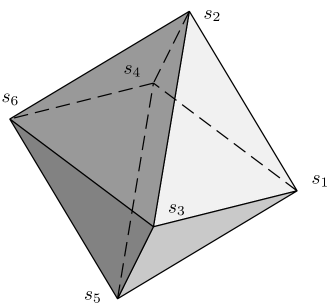
Figure 2: The octahedron graph

3.4 Consequences

By inspection, the set $\mathbb{P}=\textrm{co}\left\{\pm s_{1},\pm s_{2},\pm s_{3},\pm s_{4},\pm s_{5},\pm s_{6}\right\}$ has a non-empty interior. It is a polyhedron, with six quadrilateral and eight triangular faces. This polyhedron is a usual (a little bit elongated) triangular orthobicupola, shown at Fig. 3.

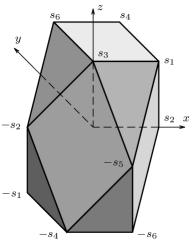
Figure 3: The polyhedron $\mathbb{P}$.

We can consider this polyhedron $\mathbb{P}$ as the unit ball in an auxiliary norm $\|\cdot\|_{*}$, in which $\|G_{n}\|_{*}\leq 1,\quad n=1,2,\ldots,12.$ Thus, the set of matrices $\{G_{n}\}$ is neutrally stable.

This implies that any product of matrices $D$, and therefore any product of matrices $B$ has only eigenvectors which are equal either to $0$ or to $1$. In particular the spectral radius of any product is equal to $1$. This proves both Proposition 6 and Proposition 4.

Now we present two interesting types of sequences of strong arbitrages, that appeared to be useful.

The sequence is $\hat{\bf A}$ is called stabilizer, if for any $\mathcal{R}$ the corresponding outcome $\hat{\bf A}\mathcal{R}$ is balanced. For example, the chain

$$\hat{\bf A}=A_{AMR}A_{FRA}A_{FMR}$$

is a stabilizer.

By definition the following assertion holds.

Lemma 1.

The chain of arbitrages is a stabilizer if and only if the product of the corresponding sequence of matrices $G$ is equal to zero.

By $\hat{\bf A}^{p}$ we denote concatenation of $p$ exemplars of $\hat{\bf A}$. For example, if $\hat{\bf A}=A_{AMR},A_{FRA},$ then

$$\hat{\bf A}^{3}=A_{AMR}A_{FRA}A_{AMR}A_{FRA}A_{AMR}A_{FRA}.$$

The chain $\hat{\bf A}$ is called destabilizer, if for some $\mathcal{R}$ all elements

$$\mathcal{R}\hat{\bf A}^{p},\quad p=1,2,\ldots,$$

are pair-wise different.

Lemma 2.

The sequence of arbitrages is a destabilizer if and only if the product of the corresponding sequence of matrices $D$ is equal an adjoint vector for the eigenvalue 1.

Follows from definitions.

The last two lemmas have been used in construction of the sequence from Proposition 3 in the following way. First, we have chosen a destabilizer given by the following chain of strong arbitrages:

$$\hat{\bf A}=\mathcal{A}_{FRM}\mathcal{A}_{FMR}\mathcal{A}_{RMA}.$$

Secondly, we multiplied it by the stabilizer

$$\hat{\bf A}=A_{AMR}A_{FRA}A_{FMR}.$$

Thirdly, we have produced the corresponding sequence of arbitrages. Finally, we found, that in our particular case this “stabilizing” part can be reduced to $\mathcal{A}_{FMA}$.

3.5 Links to the Asynchronous Systems Theory

In conclusion, we make three remarks which could be useful in investigation of systems with more than four producers.

• Construction of matrices $B_{n}$ may be interpreted as a special case of construction of mixtures of matrices in the asynchronous systems theory (see [1] or a short survey [5]). Convergence analysis for the product of matrices $B$ is analogous to analysis of absolute $r$-asymptotic stability of asynchronous system. This problem is also similar to the problem of estimating the generalized (joint) spectral radius of a family of matrices consisting of all matrices $B_{n}$.

• Since the matrices $G$ are integer, the convergence of long regular sequences to zero is similar to the well known mortality problem (see [4, 2, 3, 8]).

• In the case of matrices $G$, the subspace of common fixed points of these matrices is trivial. Moreover, this set of matrices is irreducible: they do not have common invariant subspaces. Following [6, 7] one can find an explicit estimate for norms of all products of matrices from irreducible family. Furthermore, if all entries of the matrices are integer, the question whether any sufficiently long product would equal to zero is algorithmically solvable in a finite (may be very large, but still finite) number of operations.

References

- [1] Asarin, E.A., Kozyakin, V.S., Krasnosel′skiĭ, M.A., and Kuznetsov, N.A., Analiz ustoichivosti rassinkhronizovannykh diskretnykh sistem, Moscow: Nauka, 1992, in Russian.
- [2] Blondel, V.D. and Tsitsiklis, J.N., When is a pair of matrices mortal?, Inform. Process. Lett., 1997, vol. 63, no. 5, pp. 283–286. doi:10.1016/S0020-0190(97)00123-3.
- [3] Blondel, V.D. and Tsitsiklis, J.N., The boundedness of all products of a pair of matrices is undecidable, Systems Control Lett., 2000, vol. 41, no. 2, pp. 135–140. doi:10.1016/S0167-6911(00)00049-9.
- [4] Blondel, V.D. and Tsitsiklis, J.N., A survey of computational complexity results in systems and control, Automatica J. IFAC, 2000, vol. 36, no. 9, pp. 1249–1274.
- [5] Kozyakin, V.S., Asynchronous Systems: A Short Survey and Problems, Preprint 13/2003, Boole Centre for Research in Informatics, University College Cork — National University of Ireland, Cork, May 2003.
- [6] Kozyakin, V.S., On Explicit A Priori Estimates of the Joint Spectral Radius by the Generalized Gelfand Formula, ArXiv.org e-Print archive, Oct. 2008. arXiv:0810.2157.
- [7] Kozyakin, V.S., On the Computational Aspects of the Theory of Joint Spectral Radius, DAN, 2009, vol. 427, no. 2, pp. 160–164, in Russian, translation in Doklady Mathematics 80 (2009), no. 1, 487–491. doi:10.1134/S1064562409040097.
- [8] Tsitsiklis, J.N. and Blondel, V.D., Lyapunov exponents of pairs of matrices. A correction: “The Lyapunov exponent and joint spectral radius of pairs of matrices are hard — when not impossible — to compute and to approximate”, Math. Control Signals Systems, 1997, vol. 10, no. 4, p. 381. doi:10.1007/BF01211553.