Spin selective transport through Aharonov-Bohm and Aharonov-Casher triple quantum dot systems

Abstract

We calculate the conductance through a system of three quantum dots under two different sets of conditions that lead to spin filtering effects under an applied magnetic field. In one of them, a spin is localized in one quantum dot, as proposed by Delgado et al. [Phys. Rev. Lett. 101, 226810 (2008)]. In the other one, all dots are equivalent by symmetry and the system is subject to a Rashba spin-orbit coupling. We solve the problem using a simple effective Hamiltonian for the low-energy subspace, improving the accuracy of previous results. We obtain that correlation effects related to the Kondo physics play a minor role for parameters estimated previously. Both systems lead to a magnetic field tunable “spin valve”.

I Introduction

Quantum dots (QD’s) have attracted much attention recently because of its possible numerous applications and the impressive experimental control available in manipulating microscopic parameters. It has been established that they are promising candidates in quantum information processing, with spin coherence times of several microseconds [1, 2] and fast optical initialization and control.[3, 4, 5] QD’s are also of interest in the field of spintronics (electronics based on spin).[6, 7, 8] Systems with one QD [9, 10, 11, 12] or one magnetic impurity on the (111) surface of noble metals,[13] were used to test single impurity models with strong correlations, in which the Kondo physics was clearly displayed, confirming predictions based on the Anderson model.[14, 15, 16, 17] More recently, the scaling laws in transport under an applied bias voltage in a non-equilibrium situation,[18, 19, 20, 21] quantum phase transitions,[22, 23, 24, 25, 26, 27] and the effect of hybridization in optical transitions,[3, 28, 29] are subjects of intense research.

In addition, systems of several impurities or QD’s have also attracted much attention. For example non-trivial results for the spectral density were observed when three Cr atoms are placed on the (111) surface of Au.[30, 31] Systems of two,[32, 33, 34] three,[35, 36] and more [37] QD’s have been assembled to study the effects of interdot hopping on the Kondo effect, and other physical properties driven by strong correlations. Particular systems have been proposed theoretically to tune the density of states near the Fermi energy,[38, 39] or as realizations of the two-channel Kondo model,[40, 41] the so called ionic Hubbard model,[42] and the double exchange mechanism.[43] Transport through arrays of a few QD’s [42, 44, 45, 46, 47, 48, 49, 50] and spin qubits in double QD’s [51] have been studied theoretically.

Another subject of interest are effects of interference in quantum paths and the Aharonov-Bohm effect. They have been demonstrated in mesoscopic rings with embedded QD’s.[12, 52, 53, 54] Recent experiments in semiconductor mesoscopic rings [55, 56] have shown that the conductance oscillates not only as a function of the applied magnetic field (Aharonov-Bohm effect) but also as a function of the applied electric field perpendicular to the plane of the ring (Aharonov-Casher effect [57]). In this effect, the electrons, as they move, capture a phase that depends on the spin, as a consequence of spin-orbit coupling. The main features of the experiment can be understood in a one-electron picture.[58, 59] However, when the spin-orbit coupling is smaller or of the order of the Kondo energy, the conductance should be described with a formalism that includes correlations.[49] A device of several QD’s in an Aharonov-Bohm-Casher interferometer can be used as a spin filter, since the conductance depends on spin and can be made to vanish for one spin direction.[49] Similar effects were proposed in a system of two non-interacting QD’s.[60, 61] This is an alternative to previous proposals, such as using one QD under an applied magnetic field.[62, 63] Similar calculations including spin-orbit coupling have been performed,[64, 65, 66] but a recent study indicates that this coupling works against the desired spin-filtering effects when only one QD is present in the ring.[66] Recently, it was shown that an array of QD’s which combines Dicke and Fano effects can be used as a spin filter.[39] There are also studies in Luttinger-liquid wires with impurities.[67, 68]

Delgado et al. have studied theoretically the conductance through a system of three QD’s threaded by a magnetic flux (see Fig. 1).[50] They show that tuning the on-site energies in a particular way through applied gate voltages (localizing a spin on QD 2), the device can be used as a spin filter. The authors have used a sequential tunneling approximation to calculate the conductance. This approach cannot describe the Kondo effect. In addition, from their work, it is not clear that the conductance for each spin $G_{\sigma}$ at zero temperature reaches the ideal value $G_{0}$ ($e^{2}/h$ for the symmetric case). In fact the authors assume very small lead-dot hopping $t_{LD}$ and their result for $G_{\sigma}$ is proportional to $|t_{LD}|^{2}$. This cannot be valid at very small temperature, for which (as we show in Section IV), the maximum of $G_{\sigma}$ is near $G_{0}$ independently of $t_{LD}$.

In the first part of this paper, we study the same system as Delgado et al., mapping the relevant eigenstates of the system either to an effective Anderson model or to an effective non-interacting model depending on the parameters. The conductance of the resulting model can be evaluated rigorously using known expressions.[19, 69] The conductance as a function of the gate voltage or the applied flux displays spikes reaching a value near $e^{2}/h$ when the energy necessary to transfer an electron from the leads to the three-dot system , or conversely, vanishes. In agreement with Ref. [50], the conductance is spin polarized.

In the second part of the paper we include the effect of spin-orbit coupling. We show that the spin filtering effect persists without the need of setting different on-site energies for the three QD’s, and furthermore, a small change in the applied magnetic field reverses the spin polarization of the current.

In Sections II and III we describe the model and approximations respectively. Section IV contains our results. Section V contains a summary of the results and a discussion.

II Model

The system, represented in Fig. 1, consists of an array of three QD’s threaded by a magnetic flux, attached to two conducting leads, and subject to a Rashba spin-orbit interaction. The Hamiltonian can be written in the form

$$H=H_{TQD}+H_{L}+H_{LD},$$ (1)

where the first term consists of an extended Hubbard model that describes the triple QD [48, 49, 50]

$$H_{TQD} = \sum_{i\sigma}\{E_{i\sigma}n_{i\sigma}-t\left[e^{i(\Phi_{AB}+\sigma\Phi_{AC})/N}d_{i+1\sigma}^{\dagger}d_{i\sigma}+\mathrm{H.c.}\right]\}$$ (2)

$$+\sum_{i}\{Un_{i\downarrow}n_{i\uparrow}+Vn_{i}n_{i+1}\},.$$

with $N=3$. Here $d_{i\sigma}^{{\dagger}}$ creates an electron in the QD $i$ with spin $\sigma$, $n_{i\sigma}=d_{i\sigma}^{{\dagger}}d_{i\sigma}$, and $n_{i}=n_{i\downarrow}+n_{i\uparrow}$. The phase accumulated by the hopping terms $(\Phi_{AB}+\sigma\Phi_{AC})$, $\sigma=\pm 1$, contains an Aharonov-Bohm phase $\Phi_{AB}=2\pi\phi/\phi_{0}$, where $\phi$ is the magnetic flux threading the triangle and $\phi_{0}=h/e$ is the flux quantum, as well as a spin dependent Aharonov-Casher phase [49]

$$\Phi_{AC}=\sqrt{\pi^{2}+R^{2}}-\pi,$$ (3)

where

$$R=\pi\hbar\alpha E_{z}N/(2ta),$$ (4)

with $E_{z}$ the electric field perpendicular to the plane of the triangle, $\alpha$ the Rashba spin-orbit coupling constant and $a$ the interdot distance. Note that if $\alpha\neq 0$, the spin quantization axis is tilted in the radial direction by an angle $\theta=\arctan(R/\pi)$.[49] The applied magnetic field perpendicular to the plane of the triangle originates a Zeeman term, which with the chosen quantization axis has two terms, one that splits the on-site energies

$$E_{i\sigma}=E_{i}-\sigma g\mu_{B}B(\cos\theta)/2,$$ (5)

and another spin-flip term that we can safely neglect for realistic parameters, as those given in Ref. [50]. $U$ and $V$ represent the on-site and nearest-neighbor interactions respectively.

The second term in Eq. (1) describes the non-interacting leads. Their detailed description is not important as long as they have a featureless electronic structure near the Fermi energy. We represent them as semi-infinite chains following previous works [42, 48, 50]

$$H_{L}=-t_{L}[\sum_{i=-1,\sigma}^{-\infty}\left(c_{i\sigma}^{{\dagger}}c_{i-1\sigma}+\mathrm{H.c.}\right)+\sum_{i=1,\sigma}^{+\infty}\left(c_{i\sigma}^{{\dagger}}c_{i+1\sigma}+\mathrm{H.c.}\right)].$$ (6)

The remaining term in $H$ couples leads and dots

$$H_{LD}=-t_{LD}(c_{-1\sigma}^{{\dagger}}d_{1\sigma}+c_{1\sigma}^{{\dagger}}d_{3\sigma}+\mathrm{H.c.}).$$ (7)

.

III Formalism

For week enough $t_{LD}$, as it is usually the case, an excellent approximation consists in retaining the low-energy states of $H_{TQD}$ and map the system into one effective dot, coupled to the leads. This approach has been used before for similar systems.[42, 48, 49] For transport, the most interesting case (because it leads to a larger conductance) is when the ground states of two neighboring configurations, with say $n$ and $n+1$ particles are nearly degenerate. We are assuming, without loss of generality for equilibrium, that the origin of energies is at the Fermi level. One of the simplest mappings is realized when these ground states correspond to a doublet and a singlet. Then, the resulting effective model is equivalent to an impurity Anderson model with infinite on-site repulsion.[42] Although this model is not trivial, it can be appropriately handled by different techniques [71, 72] and the conductance exhibits the characteristic features of the Kondo effect when the doublet is well below the singlet.[72] However, when quantum interference effects as those present in Aharonov-Bohm rings are important, more low-energy states should be included [70] and the effective Hamiltonian is more involved.[49]

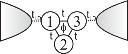
Figure 1: Scheme of the system of three QD’s coupled to two conducting leads.

In the present paper we assume that the gate voltage $V_{g}$ which shifts rigidly the on-site energies $E_{i\sigma}$ by the amount $-eV_{g}$ is such that the configurations with one and two particles are nearly degenerate. For realistic parameters,[50] we obtain that the original model can be mapped accurately into an Anderson model. Moreover, when either the magnetic field $B$ or the spin-orbit coupling $\alpha$ is large enough, one can retain only one state of both configurations and the effective model reduces to a spinless one, which can be solved trivially. Here we describe in more detail this mapping, assuming that the ground state for $n=2$ is connected adiabatically with a singlet for $\alpha=0$. This is always true for not too high magnetic field.[73] For simplicity, we also assume that the system has reflection symmetry (see Fig. 1). The generalization to other cases is straightforward and follows similar procedures as in previous papers.[42, 48, 49]

The ground state for two electrons $|2g\rangle$ is mapped into the vacuum state $|0\rangle$ of a fictitious effective QD. Similarly, the ground state for one electron $|1g\rangle$ is mapped into $\tilde{d}^{\dagger}|0\rangle$. For simplicity, in the following derivation we assume that $|1g\rangle$ has spin up (this is the case for $B>0$ and $\alpha=0$). Otherwise spin up and down should be interchanged below. Introducing hole operators $h_{j}=e^{i\varphi_{j}}c_{j\downarrow}^{{\dagger}}$ for the leads (with phases $\varphi_{j}$ chosen in such a way that $\tilde{t}_{LD}$ below is real and positive), the effective Hamiltonian takes the form

$$H_{eff} = t_{L}[\sum_{i=-1}^{-\infty}\left(h_{i}^{{\dagger}}h_{i-1}+\mathrm{H.c.}\right)+\sum_{i=1}^{+\infty}\left(h_{i}^{{\dagger}}h_{i+1}+\mathrm{H.c.}\right)]$$ (8)

$$+E_{d}\tilde{d}^{\dagger}\tilde{d}-\tilde{t}_{LD}(h_{-1}^{{\dagger}}\tilde{d}+h_{1}^{{\dagger}}\tilde{d}+\mathrm{H.c.}),$$

where

$$E_{d} = E_{1g}-E_{2g},$$

$$\tilde{t}_{LD} = t_{LD}|\langle 2g|d_{1\downarrow}^{\dagger}|1g\rangle|,$$ (9)

and $E_{ng}$ is the energy of $|ng\rangle$.

Note that the electrons that can hop to the three-dot system, rendering $|1g\rangle$ into $|2g\rangle$, have opposite spin as $|1g\rangle$. Thus the conduction for spin up is zero and the current is polarized down within this approach (due to the truncation of the Hilbert space). The validity of the approach and how this argument is modified when more states are included in the low-energy manifold, is discussed in the next section.

The spectral density at the effective dot is given by

$$\rho_{d}(\omega)=\frac{i}{2\pi}\left(\langle\langle\tilde{d};\tilde{d}^{\dagger}\rangle\rangle_{\omega+i\epsilon}-\langle\langle\tilde{d};\tilde{d}^{\dagger}\rangle\rangle_{\omega-i\epsilon}\right),$$ (10)

and the Green’s function $\langle\langle\tilde{d};\tilde{d}^{\dagger}\rangle\rangle$ can be obtained from the equations of motion. After some algebra one obtains

$$\rho_{d}(\omega)=\frac{4\tilde{t}_{LD}^{2}\left[4t_{L}^{2}-\omega^{2}\right]^{\frac{1}{2}}}{\pi\left\{\left[(\omega-E_{d})\omega-4\tilde{t}_{LD}^{2}\right]^{2}+(\omega-E_{d})^{2}\left[4t_{L}^{2}-\omega^{2}\right]\right\}}.$$ (11)

The conductance can be evaluated from this density and that of the semi-infinite chain that describes the leads,[74] using known expressions for nonequilibrium dynamics.[69, 72] In the present paper we restrict ourselves to the linear response regime and the expression for the conductance takes the form [74]

$$G=G_{0}\frac{2\pi\tilde{t}_{LD}^{2}}{t_{L}}\int\left(-\frac{\partial f}{\partial\omega}\right)\left[1-\left(\frac{\omega}{2t_{L}}\right)^{2}\right]^{\frac{1}{2}}\rho_{d}(\omega)d\omega,$$ (12)

where $G_{0}=e^{2}/h$ and $f(\omega)$ is the Fermi function.

The above expression is valid as long as for each configuration, the energy difference between excited states and the ground state is larger than $kT$ and the resonant level width $\Delta=2$ $\tilde{t}_{LD}^{2}/t_{L}$. This is the case for the parameters of the model for not too small $B$. When the magnetic field $B$ is not strong enough, the states which become Kramers degenerate with $|1g\rangle$ for $B=0$ should both be included in $H_{eff}$ and the effective model becomes equivalent to the Anderson model under an applied magnetic field. To treat this case, we use a slave-boson mean-field approximation (SBMFA) [42, 63]. The conductance at zero temperature is given by

$$G = G_{\uparrow}+G_{\downarrow},$$

$$G_{\sigma} = \frac{e^{2}}{h}\sin^{2}(\pi n_{\sigma}),.$$ (13)

where $n_{\sigma}$ is the probability of finding the lowest lying state with one particle and spin $\sigma$ in the ground state. Within the SBMFA, the $n_{\sigma}$ are calculated solving a self-consistent set of equations described in detail in Ref. [63] Since it turns out that the Anderson and Kondo physics plays a minor role in the present paper, we do not reproduce these equations here.

IV Results

As a basis for our study we have taken the parameters given by Delgado et al. [50], calculated using a method based on linear combination of harmonic orbitals and configuration interaction.[75] We set $t\simeq 0.23$ meV as the unit of energy, $U=50t$, $V=10t$, $t_{L}=100t$ and $g=0.44$. For $t_{LD}$ we have taken several values of the order of a few times $t$, leading to a resonant level width $\Delta\sim 0.01t$.

We have performed two sets of calculations. In the first one, the one-site energies $E_{i}$ are tuned in such a way that the isolated system (for $t_{LD}=0$) lies near a quadruple degeneracy point, as described by Delgado et al. [50] and the spin-orbit coupling $\alpha=0$. In this case, $E_{1}=E_{3}$, and $E_{2}-E_{1}=V-U$. In the second set, the isolated system has $C_{3}$ symmetry, and therefore, $E_{1}=E_{2}=E_{3}$, but $\alpha\neq 0$. Using an interdot distance $a=60$ nm [50] and $t=0.23$ meV, Eq. (4) gives $R\simeq\hbar\alpha E_{z}/$(3 nm meV). Typical values [76] of $\hbar\alpha E_{z}$ with an intrinsic electric field $E_{z}$ are 0.5 nm meV for GaAs [77] and 10 nm meV for InAs.[78, 79] Using externally applied $E_{z}$, the value of $R$ can be increased up to 5.[55, 56] Here we take $R$ of the order of 1, for which the mapping to an effective spinless model is valid in general.[80] For $R$ of the order of  0.1 or less, more than one state in the one-particle subspace becomes relevant and the effective Hamiltonian is more involved.[49]

IV.1 System with different on-site energies without spin-orbit coupling

Here we report the results with $\alpha=0$, $E_{1}=E_{3}$, and $E_{2}-E_{1}=V-U$.

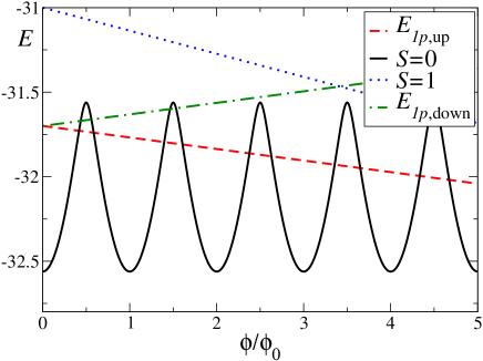
Figure 2: (Color online) Energy levels of the system as a function of the applied magnetic flux.

In Fig. 2 we show the relevant energy levels (for one and two particles in the system of three QD’s) as a function of the applied magnetic field $B$ for a gate voltage chosen in such a way that there are several crossings between the ground state for one and two particles. At these crossings one expects a large conductance,[50] and this is confirmed by our calculations described below. For two particles, the ground state is a singlet except for magnetic flux $\phi$ larger than 10 times the flux quantum $\phi_{0}=h/e$, for which the ground state becomes the triplet with projection 1.[73]

The one-particle states with lowest energy are Kramers degenerate for $B=0$ and are split by the Zeeman term for non-zero applied magnetic field. However, for small $B$, in principle both states should be retained, and the procedure used to derive Eq. (12) is in principle invalid. To test this, we have calculated the conductance of the effective impurity Anderson model (which hybridizes a doublet and a singlet via electronic transitions to or from the leads) in the SBMFA,[42, 63] mentioned briefly in the previous section. In Fig. 3 we have selected the magnetic flux that corresponds to the first crossing between the lowest energy levels for one and two particles, and for this magnetic field, we represent the conductance as a function of gate voltage. The contribution for spin down dominates the conductance. For both spins there is a peak in the conductance near the gate voltage for which an electron can be taken from the Fermi energy and added to the system with one particle, forming the singlet, without cost of energy. The asymmetry of the peaks, with an abrupt fall to zero at the right, is an artifact of the SBMFA. The dotted line corresponds to Eq. (12) in which the contribution to the conductance of the one-particle level with spin up is neglected. We can see that the contribution of the level with spin up is small even in this case.

This result confirms that when the Zeeman splitting $g\mu_{B}B$ is much larger than $\Delta=2$ $\tilde{t}_{LD}^{2}/t_{L}$, the approximation of taking only the lowest one-particle level is valid. For the case of Fig. 3 one has $g\mu_{B}B=0.117$ and $\Delta=0.098$. For all other crossings studied here, either the splitting of the one particle states is larger, or $t_{LD}$ is smaller than 4 (reducing $\Delta$). Therefore, we use this approximation, leading to Eq. (12) in the rest of this work. This is not only simpler, but also more accurate than the SBMFA when $g\mu_{B}B\gg\Delta$, in particular due to the above mentioned shortcoming of the SBMFA.

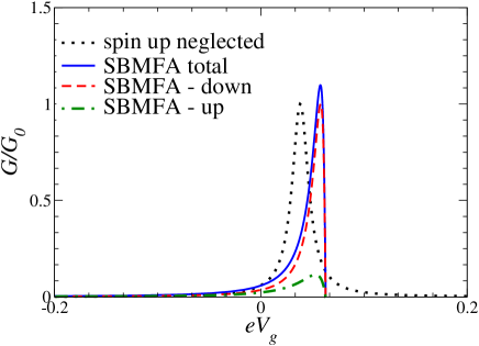
Figure 3: (Color online) Conductance for each spin as a function of gate voltage of the effective Anderson model for $t_{LD}=4.0$ and $\phi/\phi_{0}=0.43$.

Using Eq. (12), taking $t_{LD}=2$ and the rest of the parameters as in Fig. 2, we obtain the conductance as a function of flux shown in Fig. 4. As expected, there are peaks at the values of the flux which correspond to the crossing points in Fig. 2. Our results are in qualitative agreement with those of Delgado et al

In addition, our approach allows us to show that at zero temperature the height of the peaks reaches the maximum possible for given spin $G_{0}=e^{2}/h$. This ideal conductance corresponds to the symmetric case we assumed in which both leads are coupled to the dots in the same way. If not, the maximum conductance is reduced by a well known factor $A$ which depends on the difference between left and right effective couplings $\Delta$ at the Fermi energy.[19, 74]

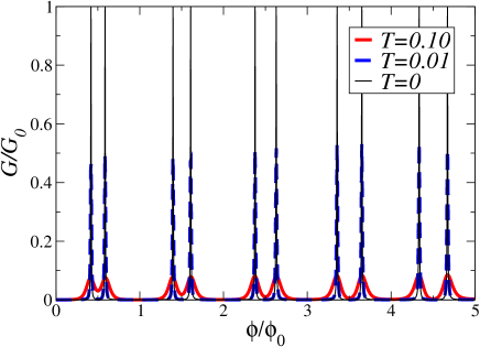
Figure 4: (Color online) Conductance as a function of the applied magnetic flux for different temperatures and for $t_{LD}=2$.

In Fig. 5 we show how the results are modified when $t_{LD}$ is increased by a factor 2, leading to a four times larger resonant level width $\Delta=2$ $\tilde{t}_{LD}^{2}/t_{L}$. As expected, the peaks are broadened and are more robust under the effect of temperature. These features might allow experimentalists an easier tuning of a spin filter device. We note that for this value $t_{LD}=4$ or higher ones, the approach of Ref. 50 predicts a conductance per spin higher than $G_{0}$. We must warn the reader that the conductance for $T=0.1$ (near 25 Kelvin) and flux near half a flux quantum are actually an underestimation, because the energy of the thermal excitation $kT$ is of the order of the Zeeman splitting $g\mu_{B}B$ and therefore both spin states contribute to the conductance.

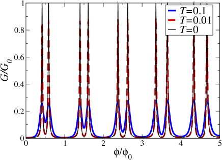
Figure 5: (Color online) Same as Fig. 4 for $t_{LD}=4$.

IV.2 System with spin-orbit coupling

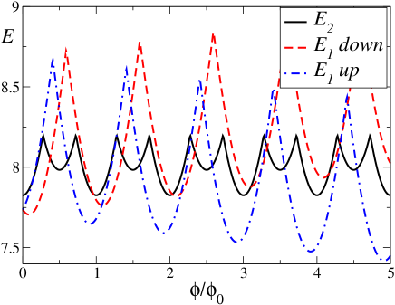
Figure 6: (Color online) Relevant energy levels as a function of the applied magnetic flux.

Here we report the results with $\alpha\neq 0$, and $E_{1}=E_{2}=E_{3}$. In Fig. 6, we show the energy of the ground state for two electrons, and the energy of the lowest-lying one-particle states, for a spin-orbit coupling such that $R=2$. The total spin ceases to be a good quantum number, but the ground state for two particles is adiabatically connected to a state that is a singlet for $R=0$, and is well separated from the states of higher energy. In contrast to the previous case, the one-particle levels now have an oscillating structure as a function of the applied magnetic field, in addition to the Zeeman splitting. This renders the maps of the crossing points more involved, with quasi-periodic changes in the spin of the one-particle ground state as the flux increases.

In any case, except at some particular points,[80] there is a spin selective conductance and as shown in Fig. 7, the peaks in which the conductance is only up or down (in the appropriate quantization axis) alternate as a function of the applied magnetic field. The broader peaks correspond to crossings of the energy levels in which the slope of the one- and two-particle levels as a function of the flux is more similar. For example, in Fig. 6, it is clear that the crossing between the energy for spin up and the two-particle state at a magnetic flux near $0.6\phi_{0}$ is more abrupt than the corresponding crossing at $\phi\sim 0.2\phi_{0}$, and as a consequence, the peak in the conductance at the former crossing is sharper (see Fig. 7).

Figure 7: (Color online) Conductance as a function of the applied magnetic flux for different temperatures, $t_{LD}=2$ and $R=2$. Top (bottom) corresponds to spin down (up).

In Fig. 8 we show the changes in the conductance for a smaller value of the spin-orbit coupling $R=1$. While the same qualitative features are retained, it becomes more difficult to separate the values of the flux for which there is a peak in the conductance for spin up or down, for small applied magnetic field. This is due to the fact that the one-particle energies for both spin directions are more similar for small applied magnetic field. For larger fields, both energies become well separated by the Zeeman term, as in the previous case.

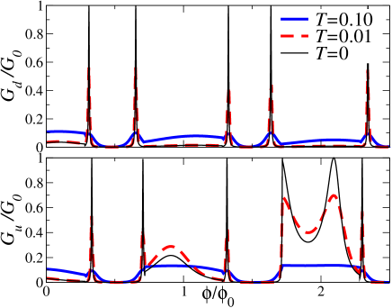
Figure 8: (Color online) Same as Fig. 7 for $R=1$

V Summary and discussion

We have investigated a system of three QD’s taking essentially parameters estimated previously,[50] for which the system acts as a magnetic field tunable spin valve. A significant spin-valve effect should be observable when either one spin is localized at the QD not connected to the leads because of its lower on-site energy combined with strong on-site Coulomb repulsion,[50] or under the effect of spin-orbit coupling.[49] In the latter case, as the magnetic flux is changed, spikes in the conductance for opposite spin orientations alternate.

While spin filtering effects in arrays of quantum dots has been studied previously,[49, 39, 50, 60, 61, 62, 63, 64, 65, 66] the fact that the effective resonant level width $\Delta$ is in general (for the given parameters) much smaller that the separation between the energy levels in the system, allows us to map the problem onto a much simpler, noninteracting one, for which the conductance can be calculated without further approximations. In particular, in spite of its simplicity, our results provide a significant quantitative improvement on those of Delgado et al.,[50] and agree with the fact that the maximum conductance per spin is the ideal one for the system $G_{0}$ independently of the lead-dot hopping $t_{LD}$.

In fact, from our study we conclude that the main ingredients to have a good spin-filtering effect is to break the Kramers degeneracy (either by an applied magnetic field on localized spins or by a spin-orbit coupling), in such a way that the separation between the low-lying levels for a configuration with $n$ electrons is larger than $\Delta$. This allows in general, the mapping to a non-interacting model. A peak in the conductance is obtained when the gate voltage is such that electrons can be transfered between both configurations without energy cost.

The most important correlations in the problem are contained in the description of the isolated system of three dots. The hybridization of the system with the leads in general introduces new effects of correlations, related with the Anderson and Kondo physics.[42, 49] However, we find that these effects are minor for the parameters used, particularly due to the breaking of the Kramers degeneracy.

Another advantage of the effective non-interacting model is that the conductance can be calculated easily in a non-equilibrium situation, as long as the applied bias voltage is small compared to the separation between low-lying energy levels in both configurations. Instead, to include non-equilibrium effects in strongly correlated models is very difficult at present.[72]

References

- [1] J. R. Petta, A. C. Johnson, J. M. Taylor, E. A. Laird, A. Yacoby, M. D. Lukin, C. M. Marcus, M. P. Hanson, and A. C. Gossard, Science 309, 2180 (2005).
- [2] A. Greilich, D. R. Yakovlev, A. Shabaev, Al. L. Efros, I. A. Yugova, R. Oulton, V. Stavarache, D. Reuter, A. Wieck, and M. Bayer, Science 313, 341 (2006).
- [3] M. Atatüre, J. Dreiser, A. Badolato, A. Högele, K. Karrai, and A. Imamoglu, Science 312, 551 (2006).
- [4] A. Greilich, R. Oulton, E. A. Zhukov, I. A. Yugova, D. R. Yakovlev, M. Bayer, A. Shabaev, Al. L. Efros, I. A. Merkulov, V. Stavarache, D. Reuter, and A. Wieck, Phys. Rev. Lett. 96, 227401 (2006).
- [5] J. Berezovsky, M. H. Mikkelsen, N. G. Stoltz, L. A. Caldren, and D. D. Awshalom, Science 320, 349 (2008).
- [6] S. Mackowski, T. Gurung, H. E. Jackson, L. M. Smith, G. Karczewski and J. Kossut, Appl. Phys. Lett. 87, 072502 (2005).
- [7] M. Korkusinski and P. Hawrylak, Phys. Rev. Lett. 101, 027205 (2008).
- [8] D. E. Reiter, T. Kuhn, and V. M. Axt, Phys. Rev. Lett. 102, 177403 (2009).
- [9] D. Goldhaber-Gordon, H. Shtrikman, D. Mahalu, D. Abusch-Magder, U. Meirav, and M. A. Kastner, Nature 391, 156 (1998).
- [10] S. M. Cronenwet, T. H. Oosterkamp, and L. P. Kouwenhoven, Science 281, 540 (1998).
- [11] D. Goldhaber-Gordon, J. Göres, M. A. Kastner, H. Shtrikman, D. Mahalu, and U. Meirav, Phys. Rev. Lett. 81, 5225 (1998).
- [12] W. G. van der Wiel, S. de Franceschi, T. Fujisawa, J. M. Elzerman, S. Tarucha, and L. P. Kowenhoven, Science 289, 2105 (2000).
- [13] H. C. Manoharan, C. P. Lutz, and D. M. Eigler, Nature (London) 403, 512 (2000); references therein.
- [14] L.I. Glazman and M.E. Raikh, JETP Lett. 47, 452 (1988).
- [15] T. K. Ng and P. A. Lee, Phys. Rev. Lett. 61, 1768 (1988).
- [16] T. A. Costi, A. C. Hewson, and V. Zlatić, J. Phys. Condens. Matter 6, 2519 (1994).
- [17] A. A. Aligia and A. M. Lobos, J. Phys.: Condens. Matter 17, S1095 (2005); references therein.
- [18] M. Grobis, I. G. Rau, R. M. Potok, H. Shtrikman, and D. Goldhaber-Gordon, Phys. Rev. Lett. 100, 246601 (2008)..
- [19] J. Rincón, A. A. Aligia, K. Hallberg, Phys. Rev. B 79, 121301(R) (2009); 80, 079902(E) (2009); 81, 039901(E) (2010.
- [20] G. D. Scott, Z. K. Keane, J. W. Ciszek, J. M. Tour, and D. Natelson, Phys. Rev. B 79, 165413 (2009).
- [21] E. Sela and J. Malecki, Phys. Rev. B 80, 233103 (2009).
- [22] N. Roch, S. Florens, V. Bouchiat, W. Wernsdorfer, and F. Balestro, Nature (London) 453, 633 (2008).
- [23] P. Roura Bas and A. A. Aligia, Phys. Rev. B 80, 035308 (2009).
- [24] D. E. Logan, C. J. Wright, and M. R. Galpin, Phys. Rev. B 80, 125117 (2009)
- [25] N. Roch, S. Florens, T. A. Costi, W. Wernsdorfer, and F. Balestro, Phys. Rev. Lett. 103, 197202 (2009).
- [26] P. Roura Bas and A. A. Aligia, J. Phys. Cond. Matt. 22, 025602 (2010).
- [27] A. K. Mitchell, T. F. Jarrold, and D. E. Logan, Phys. Rev. B 79, 085124 (2009).
- [28] P. A. Dalgarno, M. Ediger, B. D. Gerardot, J. M. Smith, S. Seidl, M. Kroner, K. Karrai, P. M. Petroff, A. O. Govorov, and R. J. Warburton, Phys. Rev. Lett. 100, 176801 (2008)
- [29] L. M. León Hilario and A. A. Aligia, Phys. Rev. Lett. 103, 156802 (2009).
- [30] T. Jamneala, V. Madhavan, and M. F. Crommie, Phys. Rev. Lett. 87, 256804 (2001).
- [31] A. A. Aligia, Phys. Rev. Lett. 96, 096804 (2006); references therein.
- [32] H. Jeong, A. M. Chang, and M. R. Meloch, Science 304, 565 (2004).
- [33] N. J. Craig, J. M. Taylor, E. A. Lester, C. M. Marcus, M. P. Hanson, and A. C. Gossard, Science 293, 2221 (2001).
- [34] J. C. Chen, A. M. Chang, and M. R. Melloch, Phys. Rev. Lett. 92, 176801 (2004).
- [35] F. R. Waugh, M. J. Berry, D. J. Mar, R. M. Westervelt, K. L. Campman, and A. C. Gossard, Phys. Rev. Lett. 75, 705 (1995).
- [36] L. Gaudreau, S. A. Studenikin, A. S. Sachrajda, P. Zawadzki, A. Kam, J. Lapointe, M. Korkusinski, and P. Hawrylak, Phys. Rev. Lett. 97, 036807 (2006).
- [37] L. P. Kouwenhoven, F. W. J. Hekking, B. J. van Wees, C. J. P. M. Harmans, C. E. Timmering, and C. T. Foxon, Phys. Rev. Lett. 65, 361 (1990).
- [38] L. G. G. V. Dias da Silva, N. P. Sandler, K. Ingersent, and S. E. Ulloa, Phys. Rev. Lett. 97, 096603 (2006); ibid 99, 209702 (2007); L. Vaugier, A.A. Aligia and A.M. Lobos, ibid 99, 209701 (2007); L. Vaugier, A.A. Aligia and A.M. Lobos, Phys. Rev. B 76, 165112 (2007).
- [39] J. H. Ojeda, M. Pacheco, and P. A. Orellana, Nanotechnology 20, 434013 (2009).
- [40] Y. Oreg and D. Goldhaber-Gordon, Phys. Rev. Lett. 90, 136602 (2003).
- [41] R. Žitko and J. Bonča, Phys. Rev. B 74, 224411 (2006).
- [42] A. A. Aligia, K. Hallberg, B. Normand, and A. P. Kampf, Phys. Rev. Lett. 93, 076801 (2004).
- [43] G. B. Martins, C. A. Büsser, K. A. Al-Hassanieh, A. Moreo, and E. Dagotto, Phys. Rev. Lett. 94, 026804 (2005).
- [44] P. S. Cornaglia and D. R. Grempel, Phys. Rev. B 71, 075305 (2005).
- [45] R. Žitko and J. Bonča, Phys. Rev. B 73, 035332 (2006).
- [46] A. Oguri , Y. Nisikawa, and A. C. Hewson, J. Phys. Soc. Jpn. 74, 2554 (2005).
- [47] Y. Nisikawa and A. Oguri, Phys. Rev. B 73, 125108 (2006).
- [48] A. M. Lobos and A. A. Aligia, Phys. Rev. B 74, 165417 (2006).
- [49] A. M. Lobos and A. A. Aligia, Phys. Rev. Lett. 100, 016803 (2008); Physica B 404, 3306 (2009).
- [50] F. Delgado, Y.-P. Shim, M. Korkusinski, L. Gaudreau, S. A. Studenikin, A. S. Sachrajda, and P. Hawrylak, Phys. Rev. Lett. 101, 226810 (2008).
- [51] A. Ramšak, J. Mravlje, R. Žitko and J. Bonča, Phys. Rev. B 74, 241305(R) (2006).
- [52] M. Zaffalon, A. Bid, M. Heiblum, D. Mahalu, and V. Umansky, Phys. Rev. Lett. 100, 226601 (2008); references therein.
- [53] Y. Ji, M. Heiblum, D. Sprinzak, D. Mahalu, and H. Shtrikman, Science 290, 779 (2000).
- [54] A.W. Holleitner, C. R. Decker, H. Qin, K. Eberl, and R. H. Blick, Phys. Rev. Lett. 87, 256802 (2001).
- [55] M. König, A. Tschetschetkin, E. M. Hankiewicz, J. Sinova, V. Hock, V. Daumer, M. Schäfer, C. R. Becker, H. Buhmann, and L. W. Molenkamp, Phys. Rev. Lett. 96, 076804 (2006).
- [56] T. Bergsten, T. Kobayashi, Y. Sekine, and J. Nitta, Phys. Rev. Lett. 97, 196803 (2006).
- [57] Y. Aharonov and A. Casher, Phys. Rev. Lett. 53, 319 (1984).
- [58] S.-Q. Shen, Z.-J. Li, and Z. Ma, Appl. Phys. Lett. 84, 996 2004).
- [59] B. Molnár, F. M. Peeters, and P. Vasilopoulos, Phys. Rev. B 69, 155335 2004).
- [60] F. Chi, J. L. Liu, and L. L. Sun, J. Appl. Phys. 101, 093704 (2007)
- [61] F. Chi and S. S. Li, J. Appl. Phys. 100, 113703 (2006).
- [62] M. E. Torio, K. Hallberg, S. Flach, A. E. Miroshnichenko, and M. Titov, Eur. Phys. J. B 37, 399 (2004).
- [63] A. A. Aligia and L. A. Salguero, Phys. Rev. B 70, 075307 (2004); 71, 169903(E) (2005).
- [64] Q.-F. Sun, J. Wang, and H. Guo, Phys. Rev. B 71, 165310 (2005).
- [65] R. J. Heary, J. E. Han, and L. Zhu, Phys. Rev. B 77, 115132 (2008).
- [66] E. Vernek, N. Sandler, and S. E. Ulloa, Phys. Rev. B 80, 041302(R) (2009).
- [67] D. Schmeltzer, A. R. Bishop, A. Saxena, and D. L. Smith, Phys. Rev. Lett. 90, 116802 (2003).
- [68] Z. Ristivojevic, G. I. Japaridze, and T. Nattermann, Phys. Rev. Lett. 104, 076401 (2010).
- [69] Y. Meir and N. S. Wingreen, Phys. Rev. Lett. 68, 2512 (1992).
- [70] J. Rincón, A. A. Aligia, and K. Hallberg, Phys. Rev. B 79, 035112 (2009).
- [71] A. C. Hewson, in The Kondo Problem to Heavy Fermions (Cambridge, University Press, 1993).
- [72] A. A. Aligia, Phys. Rev. B 74, 155125 (2006); references therein.
- [73] For high enough magnetic field , the ground state for two particles becomes a triplet with maximum spin projection if . The derivation of the appropriate effective Hamiltonian for this case, is similar to the one given in the text.
- [74] A.A. Aligia and C.R. Proetto, Phys. Rev. B 65, 165305 (2002).
- [75] I. Puerto Gimenez, M. Korkusinski, and P. Hawrylak, Phys. Rev. B 76, 075336 (2007)
- [76] G. Usaj and C. A. Balseiro, Phys. Rev. B 70, 041301(R) (2004).
- [77] J. B. Miller, D. M. Zumbühl, C. M. Marcus, Y. B. Lyanda-Geller, D. Goldhaber-Gordon, K. Campman, and A. C. Gossard, Phys. Rev. Lett. 90 076807 (2003).
- [78] J. Nitta, T. Akazaki, H. Takayanagi, and T. Enoki, Phys. Rev. Lett. 78, 1335 (1997).
- [79] D. Grundler, Phys. Rev. Lett. 84, 6074 (2000).
- [80] For those special points in which the three energy levels shown in Fig. 6 are nearly degenerate, the effective Hamiltonian (8) becomes invalid and a more elaborate formalism shold be used to calculate the conductance.[49]