Global behavior of solutions of nonlinear ODEs: first order equations

Abstract.

We determine the behavior of the general solution, small or large, of nonlinear first order ODEs in a neighborhood of an irregular singular point chosen to be infinity. We show that the solutions can be controlled in a ramified neighborhood of infinity using a finite set of asymptotic constants of motion; the asymptotic formulas can be calculated to any order by quadratures. These constants of motion enable us to obtain qualitative and accurate quantitative information on the solutions in a neighborhood of infinity, as well as to determine the position of their singularities. We discuss how the method extends to higher order equations. There are some conceptual similarities with a KAM approach, and we discuss this briefly.

1. Introduction

The point at infinity is most often an irregular singular point for equations arising in applications. Within this class of equations, there are essentially two types for which a global description of solutions exists: linear systems and integrable ones. However, in a stricter sense, even for some linear problems global questions such as explicit values of connection coefficients are still open. The behavior of the general solutions of linear ODEs has been thoroughly analyzed starting in the late 19th century, see [24] and [38] and references therein. After the pioneering work of Écalle, Ramis, Sibuya and others the description of their solutions in $\mathbb{C}$ is by now quite well understood [23, 22, 5, 6, 10, 33, 34, 16].

Integrable systems provide another important class of systems allowing for global description of solutions. The ensemble of integrable systems is a zero measure set in the parameter space of general equations: a generic small perturbation of an integrable system destroys integrability. Nonetheless, integrable equations occur remarkably often in many areas of mathematics, such as orthogonal polynomials, the analysis of the Riemann-zeta function, random matrix theory, self-similar solutions of integrable PDEs and combinatorics, cf. [8],[18]–[20], [1, 11, 12, 14, 20], [21]–[40]. However, even in integrable systems, achieving global control of solutions in a practical way is a challenging task, and it is one of the important aims of the emerging Painlevé project [9].

In nonintegrable systems, particularly near irregular singularities, our understanding is much more limited. Small solutions are given by generalized Borel summable transseries; this was discovered by Écalle in the 1980s and proved rigorously in many contexts subsequently. Transseries are essentially formal multiseries in powers of $1/x^{k_{i}}$ $e^{-\lambda_{j}x}$, and possibly $x^{-1}\log x$; see again [23, 22, 5, 6, 10, 33, 34, 16] and [15]. Here $x$ is the independent variable and $\lambda_{j}$ are eigenvalues of the linearization with the property $\mathrm{Re\,}(\lambda_{j}x)>0$. In general, only small solutions are well understood. However, for generic nonlinear systems of higher order, small solutions form lower dimensional manifolds in the space of all solutions, see, e.g., [16]. The present understanding of general nonlinear equations is thus quite limited.

We introduce a new line of approach, combining ideas from generalized Borel summability and KAM theory (see, e.g. [3]) for the analysis near infinity, chosen to be an irregular singular point, of solutions of relatively general differential equations with meromorphic coefficients. Applying the method does not require knowledge of Borel summability, transseries or KAM theory.

For small solutions, in [17] it was shown that in a region adjacent to the sector where the solution, $y$, is small, $y(x)$ is almost periodic. In this sense $y$ becomes an approximately cyclic variable. In the $x$-complex plane, the singular points of $y$ are arranged in quasi-periodic arrays as well. The analysis in [17] covers an angularly small region beyond the sector where $y$ is small. Looking directly at the asymptotics of $y$ beyond this region would require a multiscale approach: $y$ has a periodic behavior–the fast scale, with $O(1/x)$ changes in the quasi-period. Multiscale analysis is usually a quite involved procedure (see, e.g., [7]).

It is natural to make a hodograph transformation in which the dependent and independent variables are switched. As mentioned above, in the “nontrivial” regions, the dependent variable is an almost cyclic one. The setting becomes somewhat similar to a KAM one: there is an underlying completely integrable system, and one looks for persistence of invariant tori. Adiabatic invariants are simply the conserved quantities associated with these tori. Evidently there are many differences between the ODE setting and the KAM one, for instance the fact that the small parameter is “internal”, $1/x$.

In this work we restrict the analysis to first order equations, mainly to ensure a transparent and concrete analysis. In theory however, the method generalizes to equations of any order, and we touch on these issues at the end of the paper.

We look at equations which, after normalization, are of the form $dy/dx=F(z,y)$, $z=1/x$, with $g$ bi-analytic at ${\bf 0}$ and $F_{y}({\bf 0})=1$.

We show that in any sector on Riemann surfaces towards infinity, the general solution is represented by transseries and/ or, in an implicit form, by some constant of motion. In fact, on large circles around $x=0$, the solution cycles among transseries representations and ones in which constants of motion describe it accurately. The regions where these behaviors occur overlap slightly to allow for asymptotic matching (cf. Corollary 8). The connection between the large $x$ behavior and the initial condition is relatively easy to obtain.

Let $\beta=F_{zy}({\bf 0})$. The constants of motion have asymptotic expansions of the form

(1) $$C(x,y)\sim x-\beta\log x+F_{0}(y)+x^{-1}F_{1}(y)+\cdots+x^{-j}F_{j}(y)+\cdots,\ \ x\to\infty.$$

Clearly, under the assumptions above, the solution $y$ can be obtained asymptotically from (1) and the implicit function theorem. The requirement that $C$ is to leading order of the form $f_{1}(x)+f_{2}(y)$, determines $C$ up to trivial transformations, see Theorem 5 and Note 2.

The functions $F_{j}$ are shown in the proof of Theorem 5 to solve first order autonomous ODEs, and thus they can always be calculated by quadratures.

To illustrate this, we use a nonintegrable Abel equation,

(2) $$u^{\prime}=u^{3}-t.$$

We note that there is no consensus on how nonintegrabilty should be defined; for (2), it is the case that the equation passes no criterion of integrability, including the poly-Painlevé test, and that there are no solutions known, explicit or coming from, say, some associated Riemann-Hilbert reformulation.

The Abel equation has the normal form (see §4, where further details about this example are given)

(3) $$y^{\prime}+3y^{3}-\frac{1}{9}+\frac{1}{5x}y=0.$$

Regions of smallness are those for which $y$ approaches a root of $3y^{3}-1/9$; in these regions, $y$ is given by a transseries [17]. Otherwise, $y$ has an implicit representation of the form

(4) $$y=\frac{1}{3}\exp\bigg{(}-C-x+\frac{1}{5}\log x+\left(\sqrt{3}-\frac{2\sqrt{3}}{5x}\right)\arctan\left(\frac{6y+1}{\sqrt{3}}\right)\\ -\log(3y-1)+\frac{1}{2}\log(9y^{2}+3y+1))+\frac{1}{x}\left(\frac{27y^{2}}{5(1-27y^{3})}+\frac{1}{25}+O(1/x)\right)\bigg{)}+\frac{1}{3},$$

obtained by inverting an appropriate constant of motion $C$ (see (39)); for the values of $\beta,F_{0},F_{1}$ see §4.1.

While in a numerical approach to calculating solutions the precision deteriorates as $x$ becomes large, the accuracy of (1) instead, increases. In examples, even when (1) is truncated to two orders, (1) is strikingly close to the actual solution even for relatively small values of the independent variable, see e.g. Figure  4.

The procedure allows for a convenient way to link initial conditions to global asymptotic behavior, see e.g. (41).

1.1. Solvability versus integrability

First order equations for which the associated second order autonomous system is Hamiltonian are in particular integrable. Indeed, by their definition, there is a globally defined smooth $H$ with the property that $\dot{x}\frac{\partial H}{\partial x}+\dot{y}\frac{\partial H}{\partial y}=0$, that is $H(x(t),y(t))=const$, providing a closed form implicit, global representation of $y$. While the differential equation provides “infinitesimal” information, $H$ –effectively an integral– provides a global one.

Conversely, clearly, if there exists an implicit solution of the equation or indeed a smooth enough conserved quantity, the equation comes from a Hamiltonian system.

What we provide is a finite set of matching conserved quantities, analogous to an atlas of overlapping maps projecting the differential field onto the trivial one, $H^{\prime}=0$. They give, in a sense, a foliation of the phase space allowing for global control of solutions. With obvious adaptations, this picture extends to higher order systems. In integrable systems there is just one single-valued map and the field is globally rectifiable. In general, the conserved quantities may be branched and not globally defined.

1.2. Normalization and definitions

Many equations of the form $y^{\prime}=F(y,1/x)$ with $F$ analytic for small $y$ and small $1/x$ can be brought to the normal form $y^{\prime}=P_{0}(y)+Q(y,1/x)$ by systematic changes of variables, see e.g. [16], [15].

The assumptions are that $Q(y,z)$ is entire in $y$ and analytic in $z$ for small $z$, and $O(y^{2},yz^{2},z)$ for small $y$ and $z$ and that $P_{0}$ is a polynomial. We assume that the roots of $P_{0}$ are simple. It will be seen from the analysis that a more general $P_{0}$ can be accommodated. We thus write the equation as

(5) $$y^{\prime}=\sum_{k=0}^{\infty}\frac{P_{k}(y)}{x^{k}}=Q_{1}(y,1/x)=P_{0}(y)+Q(y,1/x).$$

Definition 1.

$\bullet$ A formal constant of motion of (5) for $x\to\infty$ in an unbounded domain $\mathcal{D}\subset\mathbb{C}^{2}$ or on a Riemann surface covering it, and in which to leading order in $1/x$ the variables $x$ and $y$ are separated additively is a formal series

(6) $$\tilde{C}(y,x)=A(x)+F_{0}(y)+\frac{F_{1}(y)}{x}+\cdots+\frac{F_{j}(y)}{x^{j}}+\cdots$$

such that we have

$$\frac{d}{dx}\tilde{C}(y(x),x)=O(x^{-\infty})$$

in the sense that, for any $j$, $F_{j}$ and $H_{j}$ defined by

(7) $$\frac{H_{j+1}(x,y)}{x^{j+1}}:=A^{\prime}(x)+D_{x}\left(F_{0}(y)+\frac{F_{1}(y)}{x}+\cdots+\frac{F_{j}(y)}{x^{j}}\right)$$

are uniformly bounded in $\mathcal{D}$; here $D_{x}$ is the derivative along the field,

$$D_{x}F(x,y)=\nabla F\cdot(1,Q_{1})=F_{x}(x,y)+F_{y}(x,y)Q_{1}(y,1/x).$$

See also (10) below.

$\bullet$ An actual constant of motion associated to $\tilde{C}$ in $\mathcal{D}\subset\mathbb{C}^{2}$ is a function $C$ so that $C(y,x)\sim\tilde{C}(y,x)$ as $x\to\infty$ and $\frac{d}{dx}C(y(x),x)=0$ for all solutions in $\mathcal{D}$.

Note 2.

It will be seen that there is rigidity in the form of the constant of motion: if the variables in $\tilde{C}$ are, to leading order, separated additively as in (6), then, up to trivial transformations, we must have

(8) $$A(x)=-x+a\log x$$

where $a$ is the same as the one in the transseries expansion of the solution, see Proposition 6.

1.3. Finding the terms in the expansion of $\tilde{C}$

Using (8) and truncating (6) at an arbitrary $n>2$, let

(9) $${C}_{n}(y,x)=:-x+a\log x+F_{0}(y)+\sum_{k=1}^{n}\frac{F_{k}(y)}{x^{k}}.$$

We can check that $D_{x}C_{n}$ satisfies

(10) $$D_{x}C_{n}=-1+P_{0}F_{0}^{\prime}+\frac{a+P_{1}F_{0}^{\prime}+P_{0}F_{1}^{\prime}}{x}\\ +\sum_{k=2}^{n}\frac{(1-k)F_{k-1}+\sum_{j=0}^{k}P_{k-j}F^{\prime}_{j}}{x^{k}}+\frac{-nF_{n}+\sum_{j=0}^{n}\sum_{k=0}^{\infty}P_{n+k+1-j}F^{\prime}_{j}x^{-k}}{x^{n+1}}$$

(cf. (5)) where the numerator of the last term is $H_{n}$ by definition. In order for $\tilde{C}$ to be a formal constant of motion, the coefficients of $x^{-j},j=0,1,2,\ldots$ must vanish, giving

(11) $$F_{0}^{\prime}(y) =\frac{1}{P_{0}(y)}$$

(12) $$F_{1}^{\prime}(y) =-\frac{a+P_{1}(y)F_{0}^{\prime}(y)}{P_{0}(y)}$$

(13) $$F_{k}^{\prime}(y) =\frac{(k-1)F_{k-1}(y)-\sum_{j=0}^{k-1}P_{k-j}(y)F^{\prime}_{j}(y)}{P_{0}(y)}\;\quad(2\leq k\leq n).$$

It follows in particular that $F^{\prime}_{0}\neq 0$ and $F_{0}$ is bounded in $\mathcal{D}$. In solving the differential system, the constants of integration are chosen so that $F_{k}$ are indeed uniformly bounded in $y$, see (25).

1.4. Solving for $y(x)$

The expression $C_{n}$ is an approximate constant of motion ; we thus can find an approximate solution $y_{n}$ by fixing $C_{n}=K$. We then write

(14) $$G(y;K):=F_{0}(y)-K-x+a\log x+\sum_{k=1}^{n}\frac{F_{k}(y)}{x^{k}}=0$$

and we note that in the domain relevant to us ($\mathcal{S}_{1}$, see Theorem 4 below) the analytic implicit function theorem applies since

(15) $$\frac{\partial G}{\partial y}=\frac{1}{P_{0}(y)}+\frac{1}{x}E_{1}(y,x)$$

where $P_{0}$ is away from $0$ in our domain, and for some $E_{1}$ which is bounded in $\mathcal{D}$ by (9) since $Y$ is bounded. Writing $y=y_{n}$ in (14) and using the analytic implicit function theorem, treating $1/x$ as a small parameter, we get

(16) $$y_{n}=G_{0}(x;K)+\frac{G_{1}(x;K)}{x}+\cdots+\frac{G_{n}(x;K)}{x^{n}}+\frac{\tilde{H}_{n}(x;K)}{x^{n+1}}$$

where $\tilde{H}_{n}$ and the $G_{j}$’s are bounded. In the same way it is checked that $y_{n}$ is solution of (5) up to corrections $R_{n}(x;K)/x^{n+1}$, that is, $y_{n}^{\prime}-Q_{1}(y_{n},1/x)=-R_{n}(x;K)/x^{n+1}$ where $R_{n}$ is bounded.

Let $p_{1},\ldots,p_{m}$ be the distinct roots of $P_{0}$.

Let $\mathcal{R}_{y}$ be the universal cover of $Y=\mathbb{C}\backslash\{p_{1},...,p_{m}\}$. Let $\pi:X\rightarrow Y$ be the covering map.

Definition 3.

$\bullet$ An elementary $\bf y$-path of type

$$\alpha=(\alpha_{1},...,\alpha_{m},\alpha_{m+1},\ldots,\alpha_{mk})\in\mathbb{Z}^{mk},k\in\mathbb{N}$$

is a piecewise smooth curve $\gamma$ in $\mathcal{R}_{y}$ whose image under $\pi$ turns $\alpha_{1}$ times around $p_{1}$, then $\alpha_{2}$ times around $p_{2}$, and so on, $\alpha_{m}$ times around $p_{m}$, then again $\alpha_{m+1}$ times around $p_{1}$ , etc. Note that $\alpha$ is in fact an element of the fundamental group.

$\bullet$ A $\bf y$-path of type $\boldsymbol{\alpha}$ is a smooth curve $\gamma$ obtained as an arbitrary forward concatenation of elementary $y$-paths of type $\alpha$. More precisely, a $y$-path of type $\alpha$ is a map $\gamma:[0,\infty)\to\mathcal{R}_{y}$ so that, for any $N\in\mathbb{Z}^{+}$, $\gamma|_{[N,N+1]}$ is an elementary $y$-path of type $\alpha$. We will naturally denote by $\gamma|_{[0,a]}$ subarcs of $\gamma$. We see that $y$-paths are compositions of closed loops in the complex $y$ domain.

$\bullet$ $\mathcal{S}_{r}$ is a regular domain of type $\boldsymbol{\alpha}$ or an $R$-domain of type $\alpha$, if it is an unbounded open subset of $\mathcal{R}_{y}$ that contains only images of $y$-paths of type $\alpha$. Thus the image of any unbounded $y$-path of type $\alpha^{\prime}\neq\alpha$ is not a subset of $\mathcal{S}_{r}$.

Note. In our results we only need $y$-paths with the additional property that $x(y)\to\infty$ along the path.

To take a trivial illustration, in the equation $y^{\prime}=y$ an example of a $y$-path along which $x\to\infty$ is $t\mapsto\exp(it),t\geq 0$.

2. Main results

2.1. Existence of formal constants of motion

Under the assumptions at the beginning of §1.2 we have

Theorem 4.

Let $\mathcal{S}_{y}$ be an $R$-domain of type $\alpha$, and

$$\mathcal{S}_{1}=\{y\in\mathcal{S}_{y}:|\pi(y)|<M_{0}~{}{\rm and}~{}|\pi(y)-p_{k}|>\epsilon~{}{\rm for~{}all~{}}k\}$$

where $M_{0}>0$ is an arbitrary constant. Let $\mathcal{C}$ be the union of $m$ circular paths surrounding $\alpha_{k}\in\mathbb{Z}$ times the root $p_{k}$, $k=1,\ldots,m$, chosen so that

(17) $$\int_{\mathcal{C}}\frac{1}{P_{0}(y)}dy\neq 0.$$

Then, if $R_{0}$ is large enough, there exists a formal constant of motion in

$$\mathcal{D}_{1}=\{(x,y):|x|>R_{0},y\in\mathcal{S}_{1}\}$$

of the form (6). The terms $F_{k}$ in the expansion of $\tilde{C}$ in (6) can be calculated by quadratures.

Actual constants of motion are obtained in Theorem 5.

Consider now a set $\mathcal{S}$ of curves $\gamma$, $|\gamma(t)|\to\infty$ as $t\to\infty$, with the property that for all $t_{1}<t_{2}$ and all $n$ (which is in fact equivalent to for $n=0,1$ )

(18) $$\left|\mathrm{Re\,}\displaystyle\int_{\gamma(t_{1})}^{\gamma(t_{2})}\frac{\partial}{\partial y}Q_{1}(y,\gamma(t))|_{y=y_{n}(\gamma(t))}\gamma^{\prime}(t)dt\right|\leqslant b\log(|\gamma(t_{2})/\gamma(t_{1})|+1),$$

where $b>0$ is a constant, and such that there is an $M$ so that for all $n$ we have $|y_{n}|<M$ along $\gamma$. Here $M$ can be chosen large if $x$ is large. Note that $\mathcal{S}$ contains the curves $\gamma(t)$ so that $y_{n}(\gamma(t))$ is an $\alpha$-path. Indeed, by (16) , in this case, the integrand in (18) is of the form $\frac{P_{0}^{\prime}(y)}{P_{0}(y)}dy+O(1)\frac{d\gamma(t)}{\gamma(t)}$ and hence the integral equals $2\pi iN+O(\log(|N|+1))$ for large $N$ where $N$ is the number of loops.

Theorem 5.

Assume $\tilde{C}$ in (6) is a formal constant of motion in a region $\mathcal{D}=\mathcal{S}\cap\mathcal{D}_{1}$. Then there exists an actual constant of motion $C=C(x,y)$ defined in the same region, so that $C\sim\tilde{C}$ as $x\to\infty$.

2.2. Regions where $P_{0}(u)$ is small

Assume $x_{0}$ is large and $|P_{0}(y(x_{0}))|<\epsilon$ is sufficiently small. This means that for some root $r_{k}$ of $P_{0}$ we have $|y(x_{0})-r_{k}|<\epsilon_{1}$ where $\epsilon_{1}$ is also small. Without loss of generality we can assume that $r_{k}=0$ and $x\in\mathbb{R}^{+}$ since the change of variables $y_{1}=y-r_{k}$, $x=x_{1}e^{i\phi}$ does not change the form of the equation. Assume also that after normalization the stability condition $\mathrm{Re\,}P_{0}^{\prime}(0)<0$ holds. Again without loss of generality, by taking $y_{2}=\alpha y_{1}$ we can arrange that $P_{0}^{\prime}(0)=-1$. The new function $Q$ in (5) will have the form $y^{2}Q_{1}(y,1/x)+x^{-2}Q_{2}(y,1/x)$ where $Q_{1}$ and $Q_{2}$ are analytic for small $y$ and $1/x$. As a result, the normalized equation assumes the form

(19) $$y^{\prime}=-y+f_{0}(x)+\frac{ay}{x}+y^{2}Q_{1}(y,1/x)+x^{-2}Q_{2}(y,1/x).$$

We also arrange that $f_{0}=O(x^{-M})$ as $x\to\infty$, for suitably large $M$; this is possible through a change of variables of the form $y_{2}=y_{3}+\sum_{k=1}^{M}c_{k}x^{-k}$, where the $c_{k}$’s are the coefficients of the formal power series solution for small $y$.

Proposition 6.

[see [16] Theorem 3] Any solution of (19) that is $o(1)$ as $x\to\infty$ along some ray in the right half plane can be written as a Borel summed transseries, that is

(20) $$y(x)=\sum_{k=0}^{\infty}C^{k}x^{ka+1}e^{-kx}y_{k}$$

where $y_{k}$ are generalized Borel sums of their asymptotic series, and the decomposition is unique. There exist bounds, uniform in $n$ and $x$, of the form $|y_{n}(x)|<A^{k}$, and thereby the sum converges uniformly in a region $\mathcal{R}$ that contains any sector $\mathcal{S}_{c}:=\{x:|\arg\,x|<c<\pi/2\}$. Note that Theorem 3 in [16] applies to general n-th order ODEs.

Proposition 7.

(i) If, after the normalization above, $y(x_{0})$ is small (estimates can be obtained from the proof), then $y$ is given by (20).

(ii) $C(y(x),x)$, obtained by inversion of (20) for large $x$ in the right half plane and small $y$, is a constant of motion defined for all solutions for which $y(x_{0})$ is small (cf. (i)).

Proof.

(i) We write the differential equation in the equivalent integral form

(21) $$y=F_{0}(x)+y_{0}e^{-(x-x_{0})}(x/x_{0})^{a}\\ +e^{-x}x^{a}\int_{x_{0}}^{x}e^{s}s^{-a}\left[y^{2}(s)Q_{1}(y(s),1/s)+s^{-2}Q_{2}(y(s),1/s)\right]ds,$$

where $F_{0}(x)=O(x^{-M})$ ($M$ can be chosen arbitrarily large in the normalization process, [16]) and $F_{0}(x_{0})=0$. It is straightforward to show that for (21) is contractive in the norm $\|y\|=\sup_{x\in\mathcal{S}_{c}}|x^{M-1}y(x)|$ (see the beginning of this section) and thus it has a unique solution in this space. Hence, by uniqueness, the solution of the ODE with $y(x_{0})=y_{0}$, has the property $y(x)\to 0$ as $x\to\infty$. The rest of (i) now follows from [16].

(ii) We see from Proposition 6 that $y(x;C)$ is analytic in a domain of the form $\mathcal{S}_{c}\times\mathbb{D}_{\rho}$ (As usual, $\mathbb{D}_{\rho}$ denotes the disk of radius $\rho$.) We look at the rhs of (20) as a function $H(x,C)$. It follows from [16] that $y_{1}(x)=x^{-1}(1+o(1/x))$. By uniform convergence, we clearly have

(22) $$\frac{\partial H}{\partial C}=\sum_{k=0}^{\infty}kC^{k-1}x^{ka+1}e^{-kx}y_{k}=e^{-x}x^{a}(1+o(1))\neq 0.$$

The rest follows from the implicit function theorem. ∎

As a result of Theorem 5 and Proposition 7 we have the following:

Corollary 8.

If $G_{0}$ in (16) approaches a root of $P_{0}$ and $x$ is large enough, then $y$ enters a transseries region, where the new constant is given, after normalization, by Proposition 7 (ii); thus the constants of motion in different regions match.

3. Proofs and further results

3.1. Proof of Theorem 4

Let $(x_{0},y_{0})\in\mathcal{D}_{1}$. Recalling (10), we see that (11) has the solution

$$F_{0}(y)=\int_{y_{0}}^{y}\frac{1}{P_{0}(s)}ds+c_{0}$$

(we take $c_{0}=0$ since it can be absorbed into the constant of motion). Eq. (12) gives

(23) $$F_{1}(y)=f_{1}(y)+c_{1}:=-\int_{y_{0}}^{y}\frac{a+\frac{P_{1}(s)}{P_{0}(s)}}{P_{0}(s)}ds+c_{1},$$

where to ensure boundedness of $F_{1}(y)$ as the number of loops $\to\infty$, we let

$$a=-\frac{\int_{\mathcal{C}}\frac{P_{1}(y)}{P_{0}(y)^{2}}dy}{\int_{\mathcal{C}}\frac{1}{P_{0}(y)}dy}$$

and $c_{1}$ is determined to ensure boundedness of $F_{2}$ (cf. (25)). Inductively we have

(24) $$F_{k+1}(y)=\int_{y_{0}}^{y}\frac{k(f_{k}(s)+c_{k})-\sum_{j=0}^{k}P_{{k+1}-j}(s)F^{\prime}_{j}(s)}{P_{0}(s)}ds+c_{k+1}=:f_{k+1}(y)+c_{k+1}$$

for $2\leq k+1\leq n$, and, to ensure boundedness of $F_{k+1}(y)$ as the number of loops $\to\infty$ we need to choose

(25) $$c_{k}=\dfrac{\int_{\mathcal{C}}\dfrac{-kf_{k}+\sum_{j=0}^{k}P_{k+1-j}(y)f^{\prime}_{j}(y)}{P_{0}(y)}dy}{k\int_{\mathcal{C}}\dfrac{1}{P_{0}(y)}dy}$$

for $1\leq k\leq n-1$.

It is clear by induction that every singularity of $F_{k}(y)$ is a root of $P_{0}$. To complete the proof we need to show that the $F_{k}$’s are bounded in $\mathcal{D}_{1}$:

Lemma 9.

Assume $y\in\mathcal{S}_{1}$. For $\deg(P_{0})\geq 1$ and $1\leq k\leq n$ we have

$$|F_{k}^{\prime}(y)|\lesssim k!\ \ \ \ \text{and}\ \ \ \ |F_{k}(y)|\lesssim k!(|y|+1)$$

where, as usual, $\lesssim$ means $\leq$ up to an irrelevant multiplicative constant.

Proof.

We prove the lemma by induction on $k$. Note that in (23) and (24) the integration paths can be decomposed into finitely many circular loops $\mathcal{C}$ and a ray, slightly deformed around possible singularities, which implies

$$|F_{1}(y)|\lesssim\log|y|+1\lesssim|y|+1$$

and

$$|F_{k}(y)|\lesssim\left|\int_{y_{0}}^{y}|F_{k}^{\prime}(s)|ds\right|$$

where the integration path is a straight line (possibly bent as above).

We see from (13) that

$$|F_{k}^{\prime}(y)|\lesssim\frac{(k-1)|F_{k-1}(y)|}{|P_{0}(y)|}+\sum_{j=0}^{k-1}|F_{j}^{\prime}(y)|\lesssim\frac{(k-1)|F_{k-1}(y)|}{|y|+1}+\sum_{j=0}^{k-1}|F_{j}^{\prime}(y)|.$$

The conclusion then follows by induction. Note that the the last term of (10) satisfies

$$\left|-nF_{n}+\sum_{j=0}^{n}\sum_{k=0}^{\infty}P_{n+k+1-j}F^{\prime}_{j}x^{-k}\right|\lesssim(n+1)!(|y|+1)|P_{0}(y)|$$

∎

3.2. Proof of Theorem 5

Let $y(x;K)=y_{n}(x;K)+\delta(x;K)$, where $y_{n}$ is given in (16). We seek $\delta$ so that $y$ is an exact solution of (5) in $\mathcal{D}$.

Let $\phi(y,\delta)$ be the polynomial satisfying $Q_{1}(y+\delta,x)-Q_{1}(y,x)=Q_{1,y}(y,x)\delta+\delta^{2}\phi(y,\delta,x)$ where $Q_{1,y}(y,x):=\frac{\partial Q_{1}(y,x)}{\partial y}$. We obtain

(26) $$\delta^{\prime}-\frac{b\delta}{x}-\frac{\partial Q_{1}(y,x)}{\partial y}\delta=\frac{R(x;K)}{x^{n+1}}-\frac{b\delta}{x}+\phi(y_{n},\delta,x)\delta^{2}=:E(x;\delta(x);K),$$

where $R=:R_{n}$ is defined after (16); both $R$ and $\phi$ are, by assumption, bounded. In integral form, (26) reads

(27) $$\delta(x)=\int_{\infty}^{x}\frac{x^{b}}{s^{b}}e^{\int_{s}^{x}Q_{1,y}(y_{n}(t),t)dt}E(s;\delta(s);K)ds$$

where the integrals are taken along curves in $\mathcal{D}$. Using (18) we see that (27) is contractive in the norm $\|\delta\|=\displaystyle\sup_{|x|\geqslant|x_{1}|;x\in\mathcal{D}}|x|^{n}|\delta(x)|$ in an arbitrarily large ball, if $|x_{1}|$ is large enough and $n>b2^{b+1}$.

Thus (27) has a unique solution and, of course, $\delta(x)$ is the limit of the Picard like iteration

(28) $$\delta_{0}=\int_{\infty}^{x}\frac{x^{b}}{s^{b}}e^{\int_{s}^{x}Q_{1,y}(y_{n}(t),t)dt}\frac{R(s;K)}{s^{n+1}}ds\\ \delta_{1}=\int_{\infty}^{x}\frac{x^{b}}{s^{b}}e^{\int_{s}^{x}Q_{1,y}(y_{n}(t),t)dt}E(s;\delta_{0}(s);K)ds\\ etc.$$

By (27) $\delta$ is a smooth function depending on $(x,K)$ only, and $\delta=O(x^{-n})$. Smoothness is shown as usual by bootstrapping the integral representation (27).

Now we have, by (15), $\partial_{K}y_{n}(x;K)=P_{0}(y_{n})(1+o(1))$. We can easily check that $\partial_{K}\delta(x,K)=O(x^{-n})$. This is done using essentially the same arguments employed to check contractivity of the integral equation for $\delta$ in the equation in variations for $\delta_{K}$, derived by differentiating (26) with respect to $K$. We use the implicit function theorem to solve for $K$, giving $K=K(x,y)$, a smooth function of $(x,y)$. It has the following properties: $K(x,y(x))$ is by construction constant along admissible trajectories and by straightforward verification, i.e. comparing $K$ with $\tilde{C}$, we see that it is asymptotic to $\tilde{C}$ up to $O(x^{-n})$. It is known that if a function differs from the $n$th truncate of its series by $O(x^{-n})$ for large $n$, then in fact the difference is $o(x^{-n})$ (cf. [15] Proposition 1.13 (iii)).

3.3. Position of singularities of the solution

It is convenient to introduce constants of motion specific to singular regions; they provide a practical way to determine the position of singularities, to all orders.

Definition 10.

We define a simple singular solution path $\gamma(s):[0,1)\rightarrow\mathcal{R}_{y}$ to be a piecewise smooth curve whose projection $\pi(\gamma[0,1))\in\mathbb{C}$ is unbounded but turns around every $p_{k}$ only finitely many times.

A simple singular solution domain $\mathcal{S}_{s}$ is the homotopy class of any simple singular solution path, in the sense that any two unbounded paths in $\mathcal{S}_{s}$ can be continuously deformed into each other without passing through any $p_{k}$.

Proposition 11.

Let $m_{0}=\deg(P_{0})\geq 2$, $\mathcal{S}_{s}$ be a simple singular solution domain, and $\mathcal{D}_{2}=\{(x,y):|x|>R,y\in\mathcal{S}_{s},~{}{\rm and}~{}|y-p_{k}|>\epsilon~{}{\rm for~{}all~{}}k\}$. Assume that

$$\frac{|P_{k}(y)|}{|P_{0}(y)|}\lesssim|y|^{-q}$$

for large $y$, for some $q\geq 0$ and all $k\geq 1$. Note that this needs only be true in $\mathcal{S}_{s}$, which could be an angular region.

Then there exists in $\mathcal{D}_{2}$ a formal constant of motion of the form

(29) $$\tilde{C}(y,x)=x+F_{0}(y)+\frac{F_{1}(y)}{x}+\cdots+\frac{F_{j}(y)}{x^{j}}+\cdots,$$

where $F_{k}(y)$ are single valued as $y\to\infty$. Furthermore, any simple singular solution path passing through some arbitrary $(x_{0},y_{0})$ tends to a singularity, whose position $x_{sing}$ satisfies

(30) $$x_{sing}=C_{n}(y_{0},x_{0})+O\left(\frac{1}{x_{0}^{n+1}}\right)$$

for all $n\in\mathbb{N}$, where $C_{n}$ is $\tilde{C}$ truncated to $x^{-n}$.

Moreover, if there are only finitely many nonzero $P_{k}$, then there exists in $\mathcal{D}_{2}$ a true constant of motion of the form (29), i.e. the sum is convergent for large $|x|$.

Proof.

The proof is similar to that of Theorem 4.

In order for $\tilde{C}$ to be a formal constant of motion, we must have

(31) $$F_{0}^{\prime}(y) =-\frac{1}{P_{0}(y)}$$

(32) $$F_{k}^{\prime}(y) =\frac{(k-1)F_{k-1}(y)-\sum_{j=0}^{k-1}P_{k-j}(y)F^{\prime}_{j}(y)}{P_{0}(y)}\;\quad(1\leq k\leq n).$$

We solve successively for the $F_{k}$ and obtain

$$F_{0}(y)=\int_{\infty}^{y}\frac{1}{P_{0}(s)}ds$$

where the integration path lies in $\mathcal{S}_{s}$. Clearly $F_{0}$ is bounded and single valued as $y\to\infty$.

Inductively we have

(33) $$F_{k}(y)=\int_{\infty}^{y}\frac{(k-1)F_{k-1}(s)-\sum_{j=0}^{k-1}P_{k-j}(s)F^{\prime}_{j}(s)}{P_{0}(s)}ds$$

for $1\leq k\leq n$.

To prove the rest of the proposition, we need the following lemma:

Lemma 12.

Assume that $y\in\mathcal{S}_{s}$. For $1\leq k\leq n$ we have

$$|F_{k}^{\prime}(y)|\lesssim\frac{k!}{|y|^{m_{0}+q}}$$

$$|F_{k}(y)|\lesssim\frac{k!}{|y|^{m_{0}+q-1}}$$

as $y\rightarrow\infty$.

Furthermore, if $P_{k}=0$ for $k>k_{0}>0$, then

$$|F_{k}^{\prime}(y)|\lesssim\frac{c^{k}}{|y|^{m_{0}+q}}$$

$$|F_{k}(y)|\lesssim\frac{c^{k}}{|y|^{m_{0}+q-1}}.$$

Proof.

The estimates are obtained by induction on $k$. Note that (32) implies

$$|F_{k}^{\prime}(y)|\lesssim\frac{(k-1)|F_{k-1}(y)|}{|y|^{m_{0}}}+|y|^{-q}\sum_{j=0}^{k-1}|F^{\prime}_{j}(y)|$$

provided that the assumptions of the lemma hold for $1\leq j\leq k-1$.

If $P_{k}=0$ for $k>k_{0}>0$, we again show the lemma by induction.

Assume that for $0<l\leq k$ we have

$$|F_{l}^{\prime}(y)|\leq(c_{0}l_{0})^{l}\sum_{j=1}^{l+1}\binom{l}{j-1}|y|^{-1+j(1-m_{0})-q}$$

(this is obviously true for $l=1$).

This implies

$$|F_{k}(y)|\leq(c_{0}k_{0})^{k}\sum_{j=1}^{k+1}\binom{k}{j-1}\frac{|y|^{j(1-m_{0})-q}}{j(m_{0}-1)+q}$$

Thus it follows from (32) that

$$F_{k+1}^{\prime}(y)=\frac{kF_{k}(y)-\sum_{j=\max\{k-k_{0}+1,0\}}^{k}P_{k+1-j}(y)F^{\prime}_{j}(y)}{P_{0}(y)}$$

where, by the induction assumption, the first term satisfies the estimate

(34) $$\left|\frac{kF_{k}(y)}{P_{0}(y)}\right|\leq c_{1}k\left|\frac{F_{k}(y)}{y^{m_{0}}}\right|\\ \leq c_{0}^{k}k_{0}^{k+1}c_{1}\sum_{j=2}^{k+2}\frac{(k+1)\binom{k}{j-2}}{(j-1)(m_{0}-1)}|y|^{-1+j(1-m_{0})-q}\\ \leq c_{0}^{k}k_{0}^{k+1}c_{1}\sum_{j=2}^{k+2}\binom{k+1}{j-1}|y|^{-1+j(1-m_{0})-q}$$

where $c_{0}>1+c_{1}$. Note that the last inequality follows from

$$(k+1)\binom{k}{j-2}=\binom{k+1}{j-1}(j-1).$$

The second term is easy to estimate, since it is clearly bounded by

$$k_{0}(c_{0}k_{0})^{k}\sum_{j=1}^{k+1}\binom{k}{j-1}|y|^{-1+j(1-m_{0})-q}.$$

Since $c_{1}$ is fixed, we can assume that $c_{0}>1+c_{1}$, and we have

$$|F_{k+1}^{\prime}(y)|\leq(c_{0}k_{0})^{k+1}\sum_{j=1}^{k+2}\binom{k+1}{j-1}|y|^{-1+j(1-m_{0})-q}.$$

This shows the second part of the lemma. ∎

Now since

$$|D_{x}C_{n}|=\Big{|}\frac{-nF_{n}+\sum_{j=0}^{n}\sum_{k=0}^{\infty}P_{n+k+1-j}F^{\prime}_{j}x^{-k}}{x^{n+1}}\Big{|}\lesssim\frac{|P_{0}(y)|}{|x|^{n+1}|y|^{m_{0}+q}}$$

(cf. 10), the estimate for $x_{sing}$ follows immediately from integrating $D_{x}C_{n}$ from $x_{0}$ to $x_{sing}=C_{n}(\infty,x_{sing})$ along the simple singular solution path.

∎

Remark 13.

The condition

$$\frac{|P_{k}(y)|}{|P_{0}(y)|}\lesssim|y|^{-q}$$

is not the most general one for which there exists a formal constant of motion in a simple singular domain. However, this condition is frequently satisfied by ODEs that occur in applications (see §4). In such cases we can easily use (30) to find the position of the singularity (see e.g. (41)).

4. Example: the nonintegrable Abel equation (2)

To illustrate how to obtain information of the solution of a first order ODE using Theorem 4 and Proposition 11, we take as an example the nonintegrable Abel equation (2). Normalization is achieved by the transformation $x=-(9/5)A^{2}t^{5/3}$, $A^{3}=1$, $u(t)=A^{3/5}(-135)^{1/5}x^{1/5}y(x)$ [17], yielding

(35) $$y^{\prime}=-3y^{3}+\frac{1}{9}-\frac{y}{5x}.$$

Obviously (35) satisfies the assumptions in Theorem 4 and 11, with $P_{0}(y)=-3y^{3}+\displaystyle\frac{1}{9}$ and $P_{1}(y)=-\displaystyle\frac{y}{5}$.

The three roots of $P_{0}$ are $\displaystyle\frac{1}{3},~{}\displaystyle\frac{(-1)^{2/3}}{3}$, and $\displaystyle\frac{(-1)^{4/3}}{3}$. It is known [17] that there exists a solution in the right half plane $\mathbb{H}$ that goes to the root $\displaystyle\frac{1}{3}$ as $x\to\infty$. Similarly, there are solutions that go to the other two roots in other regions, which we will explore in §4.3. In those cases, the behavior of the solution follows from Proposition 6 (see also [17]). However, there are also solutions that do not go to any of the three roots. In these cases, the formal constant of motion will be a useful tool to describe quantitatively the behavior of the solution.

4.1. Constants of motion in $R$-domains

(cf. Definition 3). First we choose an elementary solution path along which the solution $y$ to (35) turns around the root $\displaystyle\frac{1}{3}$ clockwise as shown in Fig 1 and 2.

Figure 1. Solution $y(x)$ with $y_{0}=1.1$ along the line segments from 1+5i to 1.5+50i to 1.6+120i

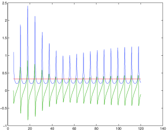
Figure 2. Real and imaginary parts of $y(x)$. The upper curve is the real part, the lower curve is the imaginary part, and the straight line is the root $1/3$.

For simplicity we calculate the first two terms of the expansion (9). We have

(36) $$F_{0}(y) =\int\frac{1}{-3y^{3}+\frac{1}{9}}dy=\sqrt{3}\arctan\left(\frac{6y+1}{\sqrt{3}}\right)-\log(3y-1)+\frac{1}{2}\log(9y^{2}+3y+1)$$

(37) $$a =\dfrac{\int_{\mathcal{C}}\frac{y}{5(-3y^{3}+\frac{1}{9})^{2}}dy}{\int_{\mathcal{C}}\frac{1}{-3y^{3}+\frac{1}{9}}dy}=\frac{1}{5}$$

(38) $$F_{1}(y) =-\int\dfrac{\frac{1}{5}-\frac{y}{5(-3y^{3}+\frac{1}{9})}}{-3y^{3}+\frac{1}{9}}dy=\frac{1}{10}\left(\frac{54y^{2}}{1-27y^{3}}-4\sqrt{3}\arctan\left(\frac{6y+1}{\sqrt{3}}\right)\right)+\frac{1}{25},$$

where the constant $\displaystyle\frac{1}{25}$ is found using (25).

We plot the first two orders of the formal constant of motion in Fig. 3.

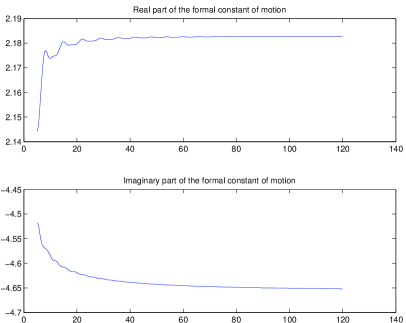
Figure 3. Formal constant of motion with $F_{0}$ and $F_{1}$.

Since this formal constant of motion is almost a constant along any path in the same $R$-domain, it can be used to find the solution asymptotically, writing

$$C=-x+\frac{1}{5}\log x+F_{0}(y)+\frac{F_{1}(y)+O(1/x)}{x}.$$

Placing the term $\log(3y-1)$ (cf. (36)) in the equation above on the left side and $C$ on the right side, taking the exponential, and solving for $y$, we obtain

(39) $$y=\frac{1}{3}\exp\bigg{(}-C-x+\frac{1}{5}\log x+\left(\sqrt{3}-\frac{2\sqrt{3}}{5x}\right)\arctan\left(\frac{6y+1}{\sqrt{3}}\right)\\ +\frac{1}{2}\log(9y^{2}+3y+1)+\frac{1}{x}\left(\frac{27y^{2}}{5(1-27y^{3})}+\frac{1}{25}+O(1/x)\right)\bigg{)}+\frac{1}{3}.$$

The reason for taking the exponential in (39) is to take care of the branching due to $\log x$, whereas the other $\log$ and $\arctan$ do not matter since the solution does not encircle their singularities. Equation (39) contains, in an implicit form, the solution $y$ to two orders in $x$. $y$ can be determined from this implicit equation in a number of ways; we chose, for simplicity to numerically solve the implicit equation using Newton’s method. The solution is plotted in Fig. 4, where we take $C=2.18-4.65i$ and calculate the solution for the second half of the path corresponding to $|x|>61.4$. Note that the relative error is within $1.5\%$.

Since the accuracy of the formal constant of motion is unaffected by going along the solution path as long as $|x|$ is large, we can obtain quantitative behavior of the solution for very large $|x|$. By contrast, in a numerical approach, the further one integrates along the path, the less accurate the calculated solution becomes.

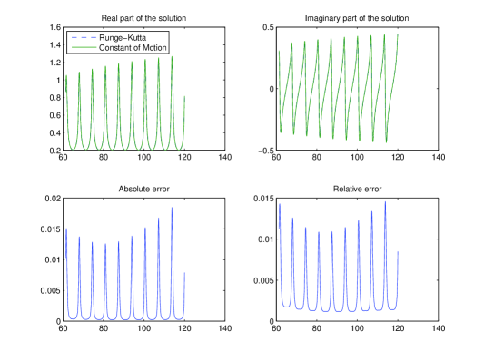
Figure 4. Comparison of solutions obtained numerically by the Runge-Kutta method and using the formal constant of motion .

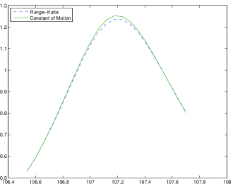
Figure 5. A small section of the left-top plot in Fig. 4.

4.2. Finding the positions of the singularities

We illustrate how to find singularities of the Abel’s equation using Proposition 11. It is known [17] that there are only square root singularities, and they appear in two arrays.

For simplicity we choose a simple singular path along which $y$ goes to $+\infty$.

According to Proposition 11 we have

(40) $$F_{0}(y)=-\int_{\infty}^{y}\frac{1}{-3s^{3}+\frac{1}{9}}ds\\ =-\sqrt{3}\arctan(\frac{6y+1}{\sqrt{3}})+\log(3y-1)-\frac{1}{2}\log(9y^{2}+3y+1)+\frac{\sqrt{3}\pi}{2}\\ F_{1}(y)=-\frac{1}{5}\int\frac{y}{(-3y^{3}+\frac{1}{9})^{2}}dy\\ =\frac{-\frac{54y^{2}}{1-27y^{3}}+2\sqrt{3}\arctan(\frac{6y+1}{\sqrt{3}})+2\log(3y-1)-\log(9y^{2}+3y+1)}{10}.$$

Thus the position of the singularity is given by the formula

(41) $$x_{1}=C+o(1)=x_{0}-\sqrt{3}\left(1-\frac{1}{5x_{0}}\right)\left(\arctan\left(\frac{6y_{0}+1}{\sqrt{3}}\right)-\frac{\pi}{2}\right)\\ +\left(1+\frac{1}{5x_{0}}\right)\left(\log(3y_{0}-1)-\frac{1}{2}\log(9y_{0}^{2}+3y_{0}+1)\right)-\frac{27y_{0}^{2}}{5x_{0}(1-27y_{0}^{3})}+o(1),$$

where the initial condition $(x_{0},y_{0})$ satisfies $|x_{0}|$ is large and $y_{0}$ is not close to any of the three roots. We note that the presence of the arctan in the leading order implies that the solutions remain quasi-periodic beyond the domain accessible to the methods in [17]. In (41) we have the freedom of choosing branch of $\log$ and $\arctan$, which enables us to find arrays of singularities.

For example, the position of a singularity corresponding to the initial condition $x_{0}=10+60i,~{}y_{0}=0.7+0.3i$, calculated using (41) is $x_{1}=9.80628+60.2167i$, which is accurate with six significant digits, as checked numerically.

The detailed behavior of the solution near the singularity can be found by expanding the right hand side of (41). We omit the calculation here since there are many other methods to determine this behavior (cf. [17]) and it is of lesser importance to the paper.

4.3. Connecting regions of transseries

We choose a path consisting of line segments The path in $x$ consists of line segments connecting $50i$, $50$, $-50i$, $-50$, $50i$, $50$, $-50i$, and $-50(\sqrt{3}+i)$. This corresponds to an angle of $2\pi$ in the original variable, with initial condition $y(50i)=0.6$.

Along this path, the solution of (35) approaches all three complex cube roots of $1/27$. For instance, the root $1/3$ is approached when $x$ traverses the first quadrant along the first segment, the root ${(-1)^{4/3}}/{3}$ is approached when $x$ goes to the lower half plane, and the root ${(-1)^{2/3}}/{3}$ is approached when $x$ goes back to the upper half plane. Some of these values are approached more than once along the entire path. This behavior can easily be shown using the phase portrait of $G_{0}$, cf. (16) and Corollary 8.

Note that along a straight line $x=x_{0}+xe^{ti}$ where the angle $t$ is fixed the leading term (with only $G_{0}$ on the right hand side) of the ODE (35) can be written as

$$\frac{dy}{dx}=e^{ti}\left(-3y^{3}-\frac{y}{5(x_{0}+xe^{ti})}+\frac{1}{9}\right).$$

Denoting $y_{1}=\mathrm{Re\,}{y}$ and $y_{2}=\mathrm{Im\,}{y}$, we have

$$\left\{\begin{array}[]{ll}\dfrac{dy_{1}}{dx}=-3y_{1}^{3}\cos t-3y_{2}^{3}\sin t+9y_{1}y_{2}^{2}\cos t+9y_{1}^{2}y_{2}\sin t+\displaystyle\frac{\cos t}{9}\\ \dfrac{dy_{2}}{dx}=-3y_{1}^{3}\sin t+3y_{2}^{3}\cos t+9y_{1}y_{2}^{2}\sin t-9y_{1}^{2}y_{2}\cos t+\displaystyle\frac{\sin t}{9}\end{array}\right.$$

We can then analyze the phase portraits. For the purpose of illustration, we show some of them in Fig 6 and 7.

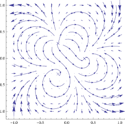
Figure 6. Phase portrait of $\mathrm{Re\,}(y)$ and $\mathrm{Im\,}(y)$ for $t=-\pi/4$. The $``\times"$ marks are the three roots.

On the line segment connecting $50i$ and $50$, it is clear that the initial condition $0.6$ is in the basin of attraction of $1/3$ (cf. Fig. 6).

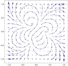
Figure 7. Phase portrait of $\mathrm{Re\,}(y)$ and $\mathrm{Im\,}(y)$ for $t=5\pi/4$.

Since the only stable equilibrium is $a_{0}=\displaystyle\frac{(-1)^{4/3}}{3}$, on the line segment connecting $50$ and $-50i$ the solution converges to $a_{0}$ (cf. Fig. 7).

Numerical calculations confirm this, (cf. Fig 8).

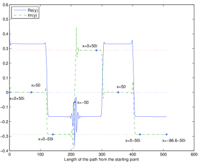
Figure 8. Behavior of the solution across transseries regions. Dotted horizontal lines are the imaginary parts of the three roots. The horizontal line is arclength. The path in $x$ consists of line segments connecting $50i$, $50$, $-50i$, $-50$, $50i$, $50$, $-50i$, and $-50(\sqrt{3}+i)$. This corresponds to an angle of $2\pi$ in the original variable.

Note 14 (Absence of limit cycles).

Finally, note that there cannot be a limit cycle in the phase portraits drawn if $x$ goes along a straight line. If the solution $y$ approaches a limit cycle, it must lie in an $R$-domain. Thus the formal constant motion formula (9) is valid, and the first term $F_{0}$ specifies a direction for $x$. If $x$ goes strictly along this direction towards $\infty$ then the term $a\log x$, which does not vanish in our case, will go to $\infty$, contradicting the results about the constant of motion. On the other hand, if $x$ goes in a different direction, then $-x+F_{0}(y)$ goes to $\infty$ much faster than $a\log x$, again a contradiction.

4.4. Extension to higher orders

For higher orders, such as the Painlevé equations P1 and P2, a similar procedure works, though the details are quite a bit more complicated, and we leave them for a subsequent work. We illustrate, without proofs, the results for $P1$, $y^{\prime\prime}=6y^{2}+z$. Now, there are two asympotic constants of motion, as expected. The normal form we work with is $u^{\prime\prime}+u^{\prime}x^{-1}-u-u^{2}/2-392x^{-4}/625=0$. Denoting by $s$ the “energy of elliptic functions” $s={u^{\prime}}^{2}/2-u^{3}/3+u^{2}$ (it turns out that $s$ is one of the bicharacteristic variables of the sequence of now PDEs governing the terms of the expansion; thus the pair $(u,s)$ is preferable to $(u,u^{\prime})$), one constant of motion has the asymptotic form

$$C_{1}=x-L(s,u)+x^{-1}K_{1}(s,u)+\cdots$$

In the above, denoting $R=\sqrt{u^{3}/3+u^{2}+s}$, $L$ is an incomplete elliptic integral, $L=\int R^{-1}(s,u)du$ and the integration is following a path winding around the zeros of $R$. The functions $K_{1}$, $K_{2}$, $\cdots$ have similar but longer expressions. We note the absence of a term of the form $a\log x$ (the reason for this is easy to see once the calculation is performed). A second constant can now be obtained by reduction of order and applying the first order techniques, or better, by the “action-angle” approach described in the introduction. It is of the form

$$C_{2}=xJ(s)+[L(s)J(u,s)-J(s)L(u,s)]+x^{-1}\tilde{K}_{1}+\cdots$$

where $J(u,s)=\int R(s,u)du$; when the variable $u$ is missing from $J(u,s)$ or $R(u,s)$, this simply means that we are dealing with complete elliptic integrals. There is directionality in the asymptotics, as the loops encircling the singularities need to be rigidly chosen according to the asymptotic direction studied. A slightly different representation allows us to calculate the constants to all orders. Because of directionality, a different asymptotic formula exists and is more useful for the “lateral connection”, that is, for calculating the solution along a circle of fixed but large radius, which will be detailed in a separate paper, as part of the Painlevé project, see e.g. [9].

5. Acknowledgments

The authors are very grateful to R. Costin for a careful reading of the manuscript and numerous useful suggestions. OC’s work was partially supported by the NSF grants DMS 0807266 and DMS 0600369.

References

- [1] Ablowitz, M., Biondini, G. Prinari, B., Inverse scattering transform for the integrable discrete nonlinear Schrödinger equation with nonvanishing boundary conditions. Inverse Problems 23, no. 4, pp. 1711–1758, (2007).
- [2] Abramowitz, M. and Stegun I.A., Handbook of Mathematical Functions with Formulas, Graphs, and Mathematical Tables, 9th printing. New York: Dover, pp. 804–806, (1972).
- [3] Arnold, V.I., Geometrical Methods in the Theory of Ordinary Differential Equations: Springer; 2nd edition (1988).
- [4] Baik, J., Buckingham, R., DiFranco, J., Its, A. Total integrals of global solutions to Painlevé II. Nonlinearity 22 no. 5, pp. 021–1061. (2009).
- [5] Balser, W., From Divergent Power Series to Analytic Functions, Springer, 1st ed. (1994).
- [6] Balser, W., Braaksma, B. L. J., Ramis, J.-P., Sibuya, Y., Multisummability of formal power series solutions of linear ordinary differential equations Asymptotic Anal. 5 no. 1, pp. 27–45. (1991).
- [7] Bender, C. and Orszag, S. Advanced Mathematical Methods for scientists and engineers, McGraw-Hill, 1978, Springer-Verlag (1999).
- [8] Bleher, P. and Its, A., Double scaling limit in the random matrix model: the Riemann-Hilbert approach. Comm. Pure Appl. Math. 56, no. 4, pp. 433–516. (2003).
- [9] Bornemann, F., Clarkson, P., Deift, P. Edelman, A., Its, A.and Lozier, D., AMS notices, V. 57, 11 p. 1389 (2010).
- [10] Braaksma, B. L. J., Multisummability of formal power series solutions of nonlinear meromorphic differential equations. Ann. Inst. Fourier no. 3, 42, pp. 517–540, (1992).
- [11] Boutet de Monvel, A., Fokas, A. S., Shepelsky, D., Integrable nonlinear evolution equations on a finite interval. Comm. Math. Phys. 263 , no. 1, pp. 133–172 (2006).
- [12] Calogero, F. A new class of solvable dynamical systems. J. Math. Phys. 49 no. 5, 052701, 9 (2008).
- [13] Clarkson, P A and Kruskal, M.D., The Painlevé-Kowalevski and poly-Painlevé tests for integrability”, Studies in Applied Mathematics 86 pp 87-165, (1992).
- [14] Conte, R., Musette, M., Verhoeven, C. Painlevé property of the Hńon-Heiles Hamiltonians. Théories asymptotiques et équations de Painlevé, pp. 65–82, Sémin. Congr., 14, Soc. Math. France, Paris, (2006).
- [15] Costin O., Asymptotics and Borel summability, Chapmann & Hall, New York (2009)
- [16] Costin O., On Borel summation and Stokes phenomena of nonlinear differential systems Duke Math. J., 93, No. 2, (1998).
- [17] Costin O. and Costin R.D., On the formation of singularities of solutions of nonlinear differential systems in antistokes directions Inventiones Mathematicae, 145, 3, pp. 425–485, (2001).
- [18] Deift, P. Four lectures on random matrix theory. Asymptotic combinatorics with applications to mathematical physics (St. Petersburg, 2001), pp. 21–52, Lecture Notes in Math., 1815, Springer, Berlin, (2003).
- [19] Baik, J., Deift, P., Johansson, K. On the distribution of the length of the longest increasing subsequence of random permutations. J. Amer. Math. Soc. 12, no. 4, pp. 1119–1178 (1999).
- [20] Deift, P.; Zhou, X. A steepest descent method for oscillatory Riemann-Hilbert problems. Asymptotics for the MKdV equation, Ann. of Math. (2) 137 no. 2, pp. 295–368, (1993).
- [21] Fokas, A. S. Soliton multidimensional equations and integrable evolutions preserving Laplace’s equation. Phys. Lett. A 372, no. 8, pp. 1277–1279, (2008).
- [22] Écalle, J., Fonctions Resurgentes, Publications Mathematiques D’Orsay, (1981).
- [23] Écalle, J., Six lectures on transseries, analysable functions and the constructive proof of Dulac’s conjecture, Bifurcations and periodic orbits of vector fields, NATO ASI Series, Vol. 408, pp. 75-184, (1993)
- [24] Fabry, C. E. Thèse (Faculté des Sciences), Paris, 1885
- [25] Fokas, A. S. Integrable nonlinear evolution equations on the half-line. Comm. Math. Phys., no. 1, pp. 1–39, 230 (2002).
- [26] Goriely, A. Integrability and nonintegrability of dynamical systems. Advanced Series in Nonlinear Dynamics, 19. World Scientific Publishing Co., Inc., River Edge, NJ, (2001).
- [27] Grammaticos, B., Ramani, A., Tamizhmani, K. M., Tamizhmani, T., Carstea, A. S. Do all integrable equations satisfy integrability criteria? Adv. Difference Equ., Art. ID 317520, (2008).
- [28] Its, A., Jimbo, M. and Maillet, J-M Integrable quantum systems and solvable statistical mechanics models. J. Math. Phys. 50, no. 9, 095101, 1 pp. 81–06, (2009)
- [29] Kruskal, M. D., Grammaticos, B., Tamizhmani, T. Three lessons on the Painlevé property and the Painlevé equations. Discrete integrable systems, 1–15, Lecture Notes in Phys., 644, Springer, Berlin (2004).
- [30] Its, A. Connection formulae for the Painlevé transcendents. The Stokes phenomenon and Hilbert’s 16th problem (Groningen, 1995), pp. 139–165, World Sci. Publ., River Edge, NJ, (1996).
- [31] Its, A. The Riemann-Hilbert problem and integrable systems. Notices Amer. Math. Soc. 50 no. 11, pp. 1389–1400 (2003).
- [32] Iwano, M., Integration analytique d’un systeme d’equations differentielles non lineaires dans le voisinage d’un point singulier, Ann. Mat. Pura Appl. (4) 44 1957, 261-292
- [33] Ramis, J-P., Gevrey, Dévissage. (French) Journées Singulières de Dijon (Univ. Dijon, Dijon, 1978), pp. 4, 173–204, Astérisque, 59-60, Soc. Math. France, Paris, (1978).
- [34] Ramis, J.-P. Les séries -sommables et leurs applications. (French) Lecture Notes in Phys., 126, pp. 178–199, Springer, Berlin-New York, (1980).
- [35] Takahashi, M., On completely integrable first order ordinary differential equations. Real and complex singularities, 388–418, World Sci. Publ., Hackensack, NJ, (2007).
- [36] Tamizhmani, K. M., Grammaticos, B., Ramani, A. Do all integrable evolution equations have the Painlevé property? SIGMA Symmetry Integrability Geom. Methods Appl. 3, Paper 073, 6 (2007).
- [37] Treves, F., Differential algebra and completely integrable systems. Hyperbolic problems and related topics, pp. 365–408, Grad. Ser. Anal., Int. Press, Somerville, MA, (2003).
- [38] Wasow, W., Asymptotic expansions for ordinary differential equations, Interscience Publishers, (1968)
- [39] Yoshino, M., Analytic non-integrable Hamiltonian systems and irregular singularity. Ann. Mat. Pura Appl. (4) 187, no. 4, pp. pp. 555–562. (2008).
- [40] Zakharov, V. E., (ed.): What is Integrability? Berlin etc., Springer-Verlag 1991