Fano Regime of Transport through Open Quantum Dots

Abstract

We analyze a quantum dot strongly coupled to the conducting leads via quantum point contacts - Fano regime of transport - and report a variety of resonant states which demonstrate the dominance of the interacting resonances in the scattering process in a low confining potential. There are resonant states similar to the eigenstates of the isolated dot, whose widths increase with increasing the coupling strength to the environment, and hybrid resonant states. The last ones are approximatively obtained as a linear combination of eigenstates with the same parity in the lateral direction, and the corresponding resonances show the phenomena of resonance trapping or level repulsion. The existence of the hybrid modes suggests that the open quantum dot behaves in the Fano regime like an artificial molecule.

I Introduction

In the past decades quantum dots were among the most studied systems in the solid state physicsFerry and Goodnick (1997); Nazarov and Blanter (2009). Proposed in the eighties as a system to minimize losses in the optical fiberKhitrova and Gibbs (2008), quantum dots have currently become a subject for fundamental research as artificial atomsKhitrova and Gibbs (2008). Here the typical properties of an isolated natural atom Kastner (1992); Ashoori (1996); Ferry and Goodnick (1997) are qualitatively reproduced even in the presence of the interaction with the environment Göres et al. (2000).

An artificial atom is a system created in a semiconductor heterostructure consisting of few electrons isolated from the environment by tunable barriersKhitrova and Gibbs (2008); Ferry and Goodnick (1997). These non-infinite barriers allow for attaching conducting leads that open the quantum dot for transport whereas the properties of the isolated dot survive to a certain degree depending on the coupling strength. From the mathematical point of view, the quantum system admits on each transport direction a continuous energy spectrum with resonances instead of a set of discrete eigenenergies. In the case of very high barriers (weak coupling) the discrete energy levels of the isolated system turn into quasi-bound states. These are isolated resonances with an extremely small imaginary part, i. e., long life-time, whose real part can be well approximated by the eigenenergies of the isolated dot Clerk et al. (2001). At weak coupling the physics of the transport phenomena is dominated by the electron-electron interaction that induces a shift of the resonant statesVasanelli et al. (2002) and the quantum dot follows the Coulomb blockade regimeFerry and Goodnick (1997); Aleiner et al. (2002). Decreasing the confinement barriers of the dot the coupling with the conducting leads increases and both, the tunneling phenomena and the spin interaction Goldhaber-Gordon et al. (1998); Avinun-Kalish et al. (2005) become more and more important relatively to the Coulomb interaction. In this intermediate regime the total transmission through the quantum dot shows broad and slightly asymmetric peaks, the so-called Kondo resonances, Goldhaber-Gordon et al. (1998); Göres et al. (2000) which are sensitive to the shape and the height of the confining barriers Vargiamidis and Potatoglou (2005). Upon further decreasing of the confining barriers the dot reaches the strong coupling regime. Here the total transmission through the quantum dot shows asymmetric peaks and dips on a slowly varying backgroundGöres et al. (2000); Kobayashi et al. (2002, 2003). These peaks exhibit a Fano line shapeFano (1961) with a complex asymmetry parameter. They are narrower compared to the ones in the intermediate regimeGöres et al. (2000). In the last years a number of studies were reported considering various specific aspects of transport in the strong coupling regime within non-interacting models Clerk et al. (2001); Racec and Wulf (2001); Racec et al. (2002); Entin-Wohlman et al. (2002); Magunov et al. (2003); Nakanishi et al. (2004); Satanin and Joe (2005); Vargiamidis and Potatoglou (2005); Mendoza et al. (2008). However, a satisfactory theory providing a complete description of the scattering mechanisms in the low confinement potentialGöres et al. (2000); Avinun-Kalish et al. (2005) at strong coupling does not exist. A particular difficulty, in this type of scattering potential is the high level density in the quantum system. As known from the particle physics, the methods used for describing quantum systems with a low level density, as the light atoms or nuclei, are not applicable for heavy nuclei with a high level densityMüller and Rotter (2009); Rotter (2009). For the mesoscopic physics, this means that the scattering problem for a quantum system in the strong coupling regime requires a different treatment compared to the scattering problem for a quantum dot in the Coulomb blockade regime.

In the strong coupling regime, the electron scattering is profoundly affected by the quantum interferencesLiu et al. (1998). The indistinguishability of the identical quantum particles leads to the interferenceLiu et al. (1998) between electrons and consequently to the Fano effectFano (1961); Fano and Rau (1986); Entin-Wohlman et al. (2002). To explain this effect, often the existence of two interfering pathways or channels is invoked, one of which is resonant while the other is non-resonant. In the experiments in Ref. [Kobayashi et al., 2002] there are two spatially well defined interference paths consisting of the two arms of the Aharonov-Bohm ring Kobayashi et al. (2002); Nakanishi et al. (2004). The arm in which a quantum dot is embedded defines the resonant path. In the experiments of Göres et al Göres et al. (2000) there are no such clearly spatially separated interference paths, and the understanding of the Fano effect in this case is not straightforward. Clerk et al Clerk et al. (2001) proposed as a nonresonant path a trajectory directly connecting the source and the drain contacts and as the resonant one a path passing through the dot via a resonant state and therefore spending a longer time in the dot. In this way, under certain conditions, the complex asymmetry parameter of a single resonance is associated with the dephasing time in the quantum system. In the frame of this model, the quite narrow and strong asymmetric (”S-type” Fano) lines are found under the assumption that the quantum dot is coupled to two single-mode leads, but the slowly varying background is not explained. In Ref. [Satanin and Joe, 2005] another model is discussed, in which the interfering paths are associated with the energy channels (subbands) of the leads: one of them contains a resonance or a group of overlapping resonances at the energy of the incoming electron while the second one contains only propagating states at this energy. As the result of the interference, asymmetric Fano lines with a complex parameter are obtained. In the presence of a scattering potential which couples the two channels it is shown that an interaction between resonances corresponding to different channels occurs, and this interaction exhibits dips in the total transmission for a favorable parity of the resonant states. As a second effect of the coupling between the scattering channels, the positions of the resonances corresponding to different channels are strongly modified in the complex energy plane. In the strong coupling regime the information about the scattering channels is actually not relevant for understanding the interaction between resonances.

The above results confirm our earlier ideaRacec and Wulf (2001) to define the interfering paths using the resonances, i. e., the complex eigenvalues of the non-Hermitian Hamilton operator of the open systemMagunov et al. (2003), instead of the quantum numbers of the lateral problem in the leads (scattering channel numbers). The resonances are also the singularities of the scattering matrix in the complex energy plane and, based on the decomposition of the $S$-matrix in a resonant and a background termRacec and Wulf (2001), we have associated the interfering paths in a more formal way with these two terms. In the limit of a quasi one-dimensional model we have proven that the Fano function with a complex asymmetry parameter arises as the most general resonance line shape under the assumption that the background can be considered constant over the width of the resonance pole. The asymmetry parameter of the Fano line reflects the strength of the interaction between the considered resonance and the background which contains the contributions of all other resonances. These results were later confirmed in Refs. [Mendoza et al., 2008; Magunov et al., 2003]. For decoupled scattering channels the Fano lines are only slightly asymmetric. The strong asymmetric ones, like those found by Göres et al Göres et al. (2000), imply the existence of many channels in the leads which can be coupled by dint of a nonseparable two-dimensional (2D) scattering potentialSatanin and Joe (2005); Mendoza et al. (2008). As mentioned in Ref. [Satanin and Joe, 2005] the interaction between channels changes the shape of the resonance dramatically.

In this paper we develop a resonant scattering theory that takes properly into account the mentioned high level density in the quantum system as well as a strong coupling of the scattering channels in a nonseparable scattering potential. In view of Ref. [Clerk et al., 2001] we assume that there exist direct trajectories which connect the source and the drain contacts, i. e., the potential energy in the region of the point contacts lies under the Fermi energy. According to the scanning electron microscope image of the systemGöres et al. (2000), the quantum point contacts are very short and the leads are wide, allowing for a few subbands. The number of the conducting channels in the source and drain contacts is essential for the coupling mechanism of the quantum dot to the contacts. In the strong coupling regime and for a quantum system with a high level density, they limit the number of the eigenstates which couple to the continuum. The other eigenstates become consequently quasi-bound statesMüller and Rotter (2009); Rotter (2009).

We believe that, for a deep understanding of the transmission through a quantum dot in the strong coupling regime, a resonant theory for two-dimensional systems is indispensable. In our opinion a resonant perturbation theory on the base of the Feshbach formalismSatanin and Joe (2005) is not sufficient for an accurate description of the strong coupling between the scattering channels. The resonances characterize the 2D scattering potential, and a direct solution of the 2D Schrödinger equation can not be avoided at least in the strong coupling regime. For this purpose we use here the R-matrix methodWigner and Eisenbud (1947); Lane and Thomas (1958); Smrčka (1990); Wulf et al. (1998); Racec and Wulf (2001); Racec et al. (2009) and extend our scattering theory for 1D systems without spherical symmetryRacec and Wulf (2001) to the case of 2D systems. The R-matrix formalism is a very powerful method which allows for an efficient procedure to determine the resonances and for an exact decomposition of the scattering matrix into resonant and nonresonant contributions around each resonanceRacec and Wulf (2001). The second advantage of using the R-matrix formalism is that the scattering theory can be extended to describe the wave functions inside the scattering area. In this way the electron probability distribution density within the dot region can be analyzed, and the resonant states can be compared with the atomic orbitals. The coupling between the scattering channels leads to the occurrence of the hybrid resonant modes. Similar hybrid modes have also been evidenced in rectangular electromagnetic resonatorsYang and Huang (2007) yielding a coupled mode with low radiation losses and a high Q-factor. As their atomic orbital counterparts, for example in $H_{2}O$-molecules, hybrid resonant modes arise in response to external perturbations of the isolated quantum system. While for atoms this perturbation consists of the molecular fields, for quantum dots the perturbation is the interaction with the conducting leads.

II The model

We provide a model for transport through a quantum dot that can be analyzed individually, like a single electron transistorKastner (1992); Goldhaber-Gordon et al. (1998); Göres et al. (2000); Avinun-Kalish et al. (2005). The dot is embedded in a quite wide and infinitely long quantum wire, isolated inside a two-dimensional electron gas (2DEG) by infinite barriers, $V(x,|y|>d_{y})\rightarrow\infty$. Inside the wire the dot is defined by the barrier $V_{b}(x,y)$, which can have a general form (nonseparable and without any symmetry) like the black area in Fig. 1. At $y=0$ there are two quantum point contacts that ensure a strong coupling between the quantum dot and the rest of the wire, which plays the role of the source and drain contacts. The contacts are characterized by constant potentials $V_{s}$ with $s=1$ for the source and $s=2$ for the drain. In the middle of the dot region the potential energy $V_{d}$ is constant and can be varied continuously by a plunger gate. Further, we make the assumption that there are no bound-states in our system, i. e., $\min[V_{1},V_{2}]=\min[V(x,y)]$, $\forall x$, $|y|<d_{y}$.

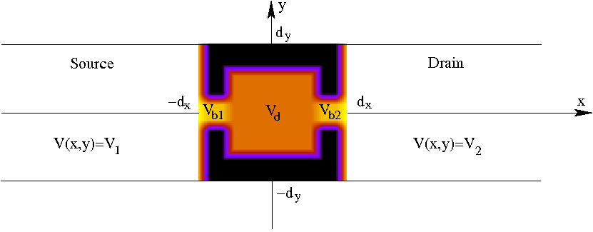
Figure 1: (Color online) Potential energy in the quantum wire: constant potential energy in the source and drain contacts, $V_{1}$ and $V_{2}$, respectively, and position dependent potential energy in the scattering region ($|x|\leq d_{x}$, $|y|\leq d_{y}$). The quantum dot is isolated inside the quantum wire by the barrier (black area) with the height $V_{b0}$ and the width $d_{b}$. The coupling between dot and contacts is set by the potential energy in the point contact regions, $V_{b1}$ and $V_{b2}$. The constant potential energy felt by the electrons inside the dot is $V_{d}$. At the interface between different domains the potential energy varies linearly with position.

The electronic wave functions are solutions of the two-dimensional Schrödinger equation

$$\left[-\frac{\hbar^{2}}{2m^{*}}\left(\frac{\partial^{2}}{\partial x^{2}}+\frac{\partial^{2}}{\partial y^{2}}\ \right)+V(x,y)\right]\;\psi(x,y)=E\;\psi(x,y),$$ (1)

with the general nonseparable potential $V(x,y)$ in the dot region; $E$ denotes here the kinetic energy of the electron in the plane of 2DEG and $m^{*}$ its effective mass. The Fermi energy Ando et al. (1982) for the 2D problem is fixed by the electron density $N_{S}$ of 2DEG, $E_{F}=\pi N_{S}\hbar^{2}/g_{v}m^{*}$, where $g_{v}$ is the valley degeneracy factor.

The electronic transport through a single quantum dot is essentially a scattering processBüttiker (1986); Büttiker et al. (1985) for which the potential energy has a spatial dependence only within a quite small region of the structure called scattering region ($|x|\leq d_{x}$, $|y|\leq d_{y}$) and is constant outside it. As usual in the scattering theory Newton (1966) this type of problem is solved using different methods for these two regions of the structure and the solutions are connected based on the continuity conditions of the wave function and its first derivative.

Outside the scattering region the Schrödinger equation is exactly solvable and, as usual in the scattering theory, those solutions are superpositions of one incident and many scattered waves,

$$\psi_{n}^{(s)}(E;x,y)=\frac{\theta(N_{s}(E)-n)}{\sqrt{2\pi}}\begin{cases}\delta_{s1}\exp{[i\;k_{1n}\;(x+d_{x})]}\;\phi_{n}(y)&\cr+\sum_{n^{\prime}=1}^{\infty}\limits\mbox{${\mathbf{\cal{S}}}$}^{T}_{sn,1n^{\prime}}(E)\exp{[-i\;k_{1n^{\prime}}\;(x+d_{x})]}\;\phi_{n^{\prime}}(y),&x\leq-d_{x}\cr\delta_{s2}\exp{[-i\;k_{2n}\;(x-d_{x})]}\;\phi_{n}(y)&\cr+\sum_{n^{\prime}=1}^{\infty}\limits\mbox{${\mathbf{\cal{S}}}$}^{T}_{sn,2n^{\prime}}(E)\exp{[i\;k_{2n^{\prime}}\;(x-d_{x})]}\;\phi_{n^{\prime}}(y),&x\geq d_{x}\end{cases}$$ (2)

$n\geq 1$, $s=1,2$, where $\theta$ denotes the step function, i. e., $\theta(t)=1$ for $t\leq 0$ and $\theta(t)=0$ for $t<0$, and $\delta_{ss^{\prime}}$ the Kronecker delta symbol, i. e., $\delta_{ss^{\prime}}=1$ for $s=s^{\prime}$ and $\delta_{ss^{\prime}}=0$ for $s\neq s^{\prime}$. The solutions (2) of the Schrödinger equation are called scattering functions and the matrix ${\mathbf{\cal{S}}}$ is the generalized scattering matrixSchanz and Smilansky (1995) or the wave transmission coefficients matrix. This is an infinite dimensional matrix, which connects incoming and outgoing components of the wave functions. $T$ denotes here the transpose matrix. Due to the electron confinement in the infinite quantum well in the $y$-direction the functions $\phi_{n}(y)$ are given as

$$\phi_{n}(y)=\frac{1}{\sqrt{d_{y}}}\sin{\left[\frac{\pi n}{2d_{y}}(y+d_{y})\right]},\quad n\geq 1$$ (3)

and the corresponding eigenenergies are

$$E_{\perp n}=\frac{\hbar^{2}}{2m^{*}}\left(\frac{\pi}{2d_{y}}\right)^{2}n^{2}.$$ (4)

The quantum numbers $n$ associated with the lateral problem define the energy channels for transport on each side of the scattering area, the so-called scattering channels. The wave vectors are defined for every channel $(sn)$ as

$$k_{sn}(E)=k_{0}\sqrt{(E-E_{\perp n}-V_{s})/u_{0}},$$ (5)

where $k_{0}=\pi/2d_{x}$ and $u_{0}=\hbar^{2}k_{0}^{2}/2m^{*}$. In the case of the conducting or open channels, $k_{sn}$ are positive real numbers, while for the non-conducting or closed channels they are given from the first branch of the complex square root function, $k_{sn}=i|k_{sn}|$. Thus, the number of the conducting channels, $N_{s}(E)$, $s=1,2$, is a function of energy, and, for a fixed energy $E$, this is the largest value of $n$ which satisfies the inequality $E-E_{\perp n}-V_{s}\geq 0$ for a given value of $s$. The scattering functions exist only for the conducting channels.

In the limit of a very low potential, i. e., $V(x,y)\rightarrow 0$, the scattering functions become plane wave corresponding to the free electrons. In the presence of a scattering potential with a non-separable character a plane wave incident onto the scattering area is reflected on every channel - open or closed for transport - of the same side of the system and transmitted on every channel - open or closed for transport - on the other side, the probability of each process being related to the elements of the generalized scattering matrix ${\mathbf{\cal{S}}}$. The $\theta$ function in Eq. (2) restricts the number of the elements with a physical meaning in ${\mathbf{\cal{S}}}$ to $N_{1}(E)+N_{2}(E)$ columns for each energy $E$.

For further determining the generalized scattering matrix ${\mathbf{\cal{S}}}$, the Schrödinger equation (1) should be also solved inside the scattering area. In this domain the potential landscape does not generally allow for analytical solutions and we have chosen to solve Eq. (1) by means of the R-matrix formalismWigner and Eisenbud (1947); Lane and Thomas (1958). Besides the extreme numerical efficiencyRacec et al. (2009), this powerful method allows for a direct comparison between the open quantum dot and its closed counterpart. In the frame of the R-matrix formalism Wigner and Eisenbud (1947); Lane and Thomas (1958); Smrčka (1990); Wulf et al. (1998); Racec and Wulf (2001); Racec et al. (2009), the scattering functions within the dot region,

$$\psi_{n}^{(s)}(E;x,y)=\sum_{l=1}^{\infty}a_{ln}^{(s)}(E)\chi_{l}(x,y),$$ (6)

$|x|\leq d_{x}$ and $|y|\leq d_{y}$, are expressed in terms of the eigenfunctions $\chi_{l}$ corresponding to the quantum dot artificially closed by Neumann boundary conditions at the interfaces with the contacts,

$$\left.\frac{\partial\chi_{l}}{\partial x}\right|_{x=\pm d_{x}}=0,$$ (7)

$l\geq 1$. Thus, the so-called Wigner-Eisenbud functions $\chi_{l}(x,y)$ satisfy the same equation as $\psi_{n}^{(s)}(x,y)$, Eq. (1), but with different boundary conditions in the transport direction: Since the scattering states $\psi_{n}^{(s)}(x,y)$ satisfy scattering, i.e. energy dependent, boundary conditions derived from Eq. (2) due to the continuity of the scattering functions at $x=\pm d_{x}$, the Wigner-Eisenbud function $\chi_{l}(x,y)$ has to satisfy energy independent boundary conditions given by Eq. (7). The infinite potential outside the quantum wire requires Dirichlet boundary condition on the surfaces perpendicular to the transport direction for both functions, $\psi_{n}^{(s)}(x,y=\pm d_{y})=0$ and $\chi_{l}(x,y=\pm d_{y})=0$. The potential energy for the Wigner-Eisenbud problem is given in Fig. 2(a). As eigenfunctions of a Hermitian Hamilton operator the functions $\chi_{l}$, $l\geq 1$, build a basis. The corresponding eigenenergies are denoted by $E_{l}$ and are called Wigner-Eisenbud energies. They are real.

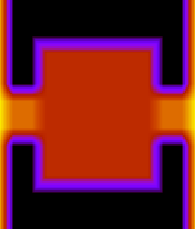
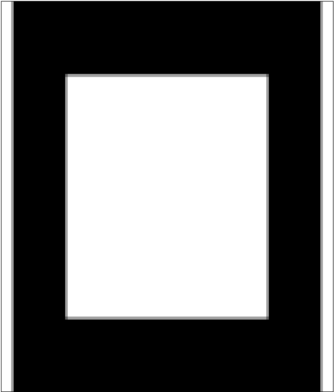
Figure 2: (Color online) (a) Closed quantum dot by means of Neumann boundary conditions at the dot-contact interfaces. This is the potential energy for the Wigner-Eisenbud problem. (b) Isolated counterpart of the considered open quantum dot ($V_{b}=V_{b1}=V_{b2}\rightarrow\infty$).

The expansion coefficients $a_{ln}^{(s)}(E)$ are calculated using the Wigner Eisenbud eigenvalue problem and the boundary conditions satisfied by the scattering functions at the interface with the contacts. We have presented this method in detail in Ref. [Racec et al., 2009]. The coefficients $a_{ln}^{(s)}(E)$ are obtained as a function of ${\mathbf{\cal{S}}}$ and the scattering functions within the dot region have the expression

$$\vec{\Psi}(E;x,y)=\frac{i}{\sqrt{2\pi}}\mathbf{\Theta}(E)[{\bf 1}-\mbox{${\mathbf{\cal{S}}}$}^{T}(E)]\mathbf{K}(E)\vec{R}(E;x,y)$$ (8)

with $\psi_{n}^{(s)}(E;x,y)=\left(\vec{\Psi}(E;x,y)\right)_{sn}$, $n\geq 1$, $s=1,2$, and the R vector defined as

$$\vec{R}(E;x,y)=\frac{u_{0}}{\sqrt{k_{0}}}\sum_{l=1}^{\infty}\frac{\chi_{l}(x,y)\vec{\chi}_{l}}{E-E_{l}}.$$ (9)

The vector $\vec{\chi}_{l}$ in Eq. (9) is constructed using the Wigner-Eisenbud functions at $x=\pm d_{x}$ and the eigenmodes corresponding to the lateral problem in the contacts,

$$(\vec{\chi_{l}})_{sn}=\frac{1}{\sqrt{k_{0}}}\int_{-d_{y}}^{d_{y}}dy\;\chi_{l}((-1)^{s}d_{x},y)\phi_{n}(y),$$ (10)

$n\geq 1,s=1,2$. The wave vectors $k_{sn}$ define the diagonal matrix $\mathbf{K}$,

$$\mathbf{K}_{sn,s^{\prime}n^{\prime}}(E)=\frac{k_{sn}(E)}{k_{0}}\,\delta_{nn^{\prime}}\delta_{ss^{\prime}},$$ (11)

$n,n^{\prime}\geq 1$, $s,s^{\prime}=1,2$. The matrix $\mathbf{\Theta}$ is also a diagonal one, defined as $\mathbf{\Theta}_{sn,s^{\prime}n^{\prime}}(E)=\theta(N_{s}(E)-n)\,\delta_{ss^{\prime}}\,\delta_{nn^{\prime}}$, $n\geq 1$, $s=1,2$.

Using further the continuity of the scattering functions on the surface of the scattering area one can derive a relation between the $\mathbf{R}$-matrix

$$\mathbf{R}(E)=u_{0}\sum_{l=1}^{\infty}\frac{\vec{\chi}_{l}\,\vec{\chi}_{l}^{T}}{E-E_{l}}$$ (12)

and the generalized scattering matrix ${\mathbf{\cal{S}}}$,

$$\mbox{${\mathbf{\cal{S}}}$}(E)=\left[\mathbf{1}-2\left(\mathbf{1}+i\mathbf{R}\mathbf{K}\right)^{-1}\right]\mathbf{\Theta}(E).$$ (13)

The equation (13) is the key relation for solving 2D scattering problems using only the eigenfunctions and the eigenenergies of the closed quantum dot [see Fig. 2(a)]. They contain the information about the scattering potential in the dot region and carry it over to the $\mathbf{R}$-matrix. The matrix $\mathbf{K}$ characterizes the contacts and can be constructed using only the constant values of the potential in these regions. On the base of Eq. (13) the generalized scattering matrix ${\mathbf{\cal{S}}}$ is calculated and further the scattering functions in each point of the system are determined using Eqs. (2) and (8). The scattering theory together with the R-matrix formalism allows for a complete description of the open quantum dot and each physical parameter of the system can be further derived from the ${\mathbf{\cal{S}}}$-matrix.

According to Eq. (12), $\mathbf{R}(E)$ is an infinite-dimensional symmetrical real matrix and its expression allows for a very efficient numerical implementation for computing it. The big advantage of the R-matrix formalism is that, for a given potential landscape, only one eigenvalue problem with energy independent boundary conditions, i. e. Wigner-Eisenbud problem, has to be numerically solved and after that the generalized scattering matrix ${\mathbf{\cal{S}}}$ can be constructed for each energy using Eq. (13). The computational costs are in this case minimal, but most important is that Eq. (13) gives the explicit dependence of ${\mathbf{\cal{S}}}$ on energy. This allows for an analysis of the scattering matrix and, after that, of the physical properties of the system, in terms of resonance energies.

The generalized scattering matrix ${\mathbf{\cal{S}}}$ describes the scattering processes not only in the asymptotic region, but also inside the scattering area. But this matrix is neither symmetric nor unitary as can be seen from Eq. (13). Further, we define the current scattering matrix as

$${\tilde{\mbox{${\mathbf{\cal{S}}}$}}}=\mathbf{K}^{1/2}\mathbf{\Theta}\mbox{${\mathbf{\cal{S}}}$}\mathbf{K}^{-1/2}.$$ (14)

The diagonal $\mathbf{\Theta}$-matrix in the above expression ensure nonzero values only for the matrix elements of $\tilde{\mbox{${\mathbf{\cal{S}}}$}}$ that correspond to conducting channels for which the transmitted flux is nonzero. For simplicity, we have dropped in (14) the energy dependence of the matrixes and we will do this often henceforth. Using the $R$-matrix representation of ${\mathbf{\cal{S}}}$, Eq. (13), the current scattering matrix becomes

$${\tilde{\mbox{${\mathbf{\cal{S}}}$}}}=\mathbf{\Theta}\left[\mathbf{1}-2(\mathbf{1}+i\mathbf{\Omega})^{-1}\right]\mathbf{\Theta},$$ (15)

with the symmetrical infinite matrix $\mathbf{\Omega}$

$$\mathbf{\Omega}(E)=u_{0}\sum_{l=1}^{\infty}\frac{\vec{\alpha}_{l}\,\vec{\alpha}^{T}_{l}}{E-E_{l}}$$ (16)

and the column vector

$$\vec{\alpha}_{l}(E)=\mathbf{K}^{1/2}\,\vec{\chi}_{l},$$ (17)

$l\geq 1$. According to Eq. (15) the current scattering matrix ${\tilde{\mbox{${\mathbf{\cal{S}}}$}}}$ is also symmetric, ${\tilde{\mbox{${\mathbf{\cal{S}}}$}}}={\tilde{\mbox{${\mathbf{\cal{S}}}$}}}^{T}$. The restriction of $\tilde{\mbox{${\mathbf{\cal{S}}}$}}$-matrix to the conducting channels is the well known current transmission matrix Wulf et al. (1998); Racec and Wulf (2001); Racec et al. (2009), $\tilde{S}$, commonly used in the Landauer-Büttiker formalism. For a given energy $E$ this is a $(N_{1}+N_{2})\times(N_{1}+N_{2})$ matrix which has to satisfy the unitarity condition $\tilde{S}\tilde{S}^{\dagger}=\tilde{S}^{\dagger}\tilde{S}={\mbox{1}}$ according to the flux conservationSchanz and Smilansky (1995).

The elements of the current transmission matrix give directly the reflection and transmission probabilities through the quantum dot. For an electron incident from the contact $s=1,2$ on the channel $n$ the probability to be transmitted into the contact $s^{\prime}\neq s$ on the channel $n^{\prime}$ is $T_{nn^{\prime}}(E)=\left|{\tilde{\mbox{${\mathbf{\cal{S}}}$}}}_{2n^{\prime},1n}(E)\right|^{2}=\left|{\tilde{\mbox{${\mathbf{\cal{S}}}$}}}_{1n^{\prime},2n}(E)\right|^{2}$. In the case of non-conducting (evanescent) channels these probabilities are zero. With these considerations, the total transmission through the dot, defined as

$$T(E)=\sum_{n=1}^{N_{1}(E)}\,\sum_{n^{\prime}=1}^{N_{2}(E)}T_{nn^{\prime}}(E),$$ (18)

becomes

$$T(E)=\mbox{Tr}[\mbox{\boldmath$\sigma$}(E)\mbox{\boldmath$\sigma$}^{\dagger}(E)],$$ (19)

where $\sigma$ is the part of $\tilde{\mbox{${\mathbf{\cal{S}}}$}}$ which contains the transmission amplitudes, $\mbox{\boldmath$\sigma$}_{nn^{\prime}}(E)=\tilde{\mbox{${\mathbf{\cal{S}}}$}}_{2n^{\prime},1n}(E)$, and $\mbox{\boldmath$\sigma$}^{\dagger}$ its adjoint.

III Resonances

The experimental analysis of a quantum system by coupling it to an electrical circuit has as a consequence the modification of its state. The physical interpretation of the measured quantities cannot be based solely on the properties of the isolated quantum system, but rather on the properties of the open system, i. e., the quantum system coupled to the contacts. Due to this coupling, the eigenstates become resonant states, some of them are long-lived resonances (called simply resonances) corresponding to quasi-bound statesFerry and Goodnick (1997); Rotter (2009) and the other ones are practically delocalizedFerry and Goodnick (1997); Rotter (2009). They can be found as states with a short life-time and it has to be elucidated if they influence significantly the physical properties or not. In addition, the resonant states are eigenstates of the non-Hermitian Hamilton operatorMüller and Rotter (2009); Rotter (2009) of the open quantum system, and they are not orthogonal to each other anymoreMüller and Rotter (2009); Rotter (2009). In principle they can interact and their coupling may also influence the physical properties.

From the mathematical point of view the resonances are associated with singularities of the current scattering matrix $\tilde{\cal{S}}$. The representation of the $\tilde{\mbox{${\mathbf{\cal{S}}}$}}$-matrix in terms of $\mathbf{\Omega}$, Eq. (15), allows for a very fast and efficient numerical procedure to determine its poles. When the quantum dot becomes open, the real eigenenergies of the closed system, $E_{l}$, migrate in the lower part of the complex energy plane, becoming resonant energiesBohm (1993), $\bar{E}_{0l}=E_{0l}-i\Gamma_{l}/2$, $l\leq 1$. Based on this correspondence, we fix an energy $E_{\lambda}$ of the closed quantum dot and determine the resonance energy $\bar{E}_{0\lambda}$ as a solution of the equation $\det[\mathbf{1}+i\mathbf{\Omega}(E)]=0$. The matrix $\Omega$, Eq. (16), is split into a $\lambda$-dependent part and a rest $\mathbf{\Omega}_{\lambda}$ which should be a slowly varying energy function at least around an isolated resonance,

$$\mathbf{\Omega}(E)=u_{0}\frac{\vec{\alpha}_{\lambda}\,\vec{\alpha}^{T}_{\lambda}}{E-E_{\lambda}}+\mathbf{\Omega}_{\lambda}(E).$$ (20)

As shown in Appendix A, this decomposition of $\mathbf{\Omega}$ around the resonance $\lambda$ leads to an expression of the $\tilde{\mbox{${\mathbf{\cal{S}}}$}}$ matrix in which the resonant and the background parts are separated

$${\tilde{\mbox{${\mathbf{\cal{S}}}$}}}(E)=2iu_{0}\frac{\mathbf{\Theta}\,\vec{\beta}_{\lambda}\,\vec{\beta}^{T}_{\lambda}\,\mathbf{\Theta}}{E-E_{\lambda}-\bar{\cal{E}}_{\lambda}}+{\tilde{\mbox{${\mathbf{\cal{S}}}$}}}_{\lambda}(E),$$ (21)

where

$$\vec{\beta}_{\lambda}(E)=(\mathbf{1}+i\mathbf{\Omega}_{\lambda})^{-1}\vec{\alpha}_{\lambda}$$ (22)

is an infinite column vector that characterizes the resonance $\lambda$,

$$\bar{\cal{E}}_{\lambda}(E)=-i\vec{\alpha}_{\lambda}\cdot\vec{\beta}^{T}_{\lambda}$$ (23)

is a complex function which assures the analyticity of the current scattering matrix for every real energy and

$${\tilde{\mbox{${\mathbf{\cal{S}}}$}}}_{\lambda}(E)=\mathbf{\Theta}\left[\mathbf{1}-2(\mathbf{1}+i\mathbf{\Omega}_{\lambda})^{-1}\right]\mathbf{\Theta}$$ (24)

is the background matrix. We have already proposed in Ref. [Racec and Wulf, 2001] a decomposition of the scattering matrix similar to Eq. (21), but for an effective one-dimensional scattering system without channel mixing. There, the $\Omega$-matrix is a $2\times 2$ one and the inversion of $1+i\Omega$ reduces to a simple algebraic calculation. In the presence of channel coupling the inversion of an infinite matrix was a real mathematical challenge (see Appendix A).

Based on the expression (21) of the scattering matrix, a resonant theory of transport through open quantum systems can be developed. Eq. (21) allows for the calculation of the resonance energies and for the analysis of each resonant contribution to the conductance. A similar decomposition of the transmission coefficient in a resonant term and a background is also proposed in Ref. [Mendoza et al., 2008], but in that case the two contributions can be evaluated provided that the eigenvalue problem for the effective Hamiltonian of the open system is already solved.

Based on Eq. (21), the position of the resonance $\bar{E}_{0\lambda}=E_{0\lambda}-i\Gamma/2$ in the complex energy plane is given as a solution of the equation

$$\bar{E}-E_{\lambda}-\bar{\cal{E}}_{\lambda}(\bar{E})=0,$$ (25)

which can be solved numerically very fast using an iterative procedure starting with $\bar{E}=E_{\lambda}$. The complex function ${\bar{\cal{E}}}_{\lambda}(E)$, Eq. (23), contains contributions from all Wigner-Eisenbud energies and from all scattering channels, i. e., all matrix elements of $\mathbf{K}$. Thus, the resonance energy $\bar{E}_{0\lambda}$ can totally differ from $E_{\lambda}$ and only in the case of a very low coupling of the dot to the contacts, $E_{\lambda}$ can properly approximate the real part of the resonance energy $\bar{E}_{0\lambda}$. With each resonance one can associate a resonance domain, which is a circle of radius $\Gamma_{\lambda}$ around $\bar{E}_{0\lambda}$ in the complex energy plane. The resonance energies for the quantum dot shown in Fig. 1 are plotted in Fig. 3 together with the Wigner-Eisenbud energies. The geometrical parameters used for the numerical calculations were taken from the electron micrograph of the single electron transistor (SET) analyzed in Ref. [Göres et al., 2000]: $2d_{x}=2d_{y}=175$ nm, $d_{b}\simeq 35$ nm so that the electrons are confined within a domain of about $100$ nm in diameter and the point contact regions are about 35 nm $\times$ 35 nm. The density of 2DEG is $N_{S}=8.1\times 10^{11}$ cm^-2 and the Fermi energy $E_{F}=29,6$ meV. The confining barrier was considered $V_{b0}=100$ meV and in the point contact regions it was taken $V_{b1}=V_{b2}=2.5$ meV; In the source and drain contacts $V_{1}\simeq V_{2}=0$. At each interface between two domains the potential energy varies linearly within a distance of 10 nm. For the numerical calculation we fixed the number of the scattering channels to $N_{1}=N_{2}=N_{F}=12$, where $N_{F}$ is the number of the conducting channels at the Fermi energy. The analyzed scattering potential is not attractive and, in turn, it is not expected that the evanescent channels play an important roleSimon (1976). Numerically, the inclusion of the evanescent channels has not produced significant variations of the conductance. In Ref. [Racec et al., 2009] a detailed discussion is presented about the scattering potentials that allow for evanescent modes and about the influence of these modes on the total transmission through an open quantum system.

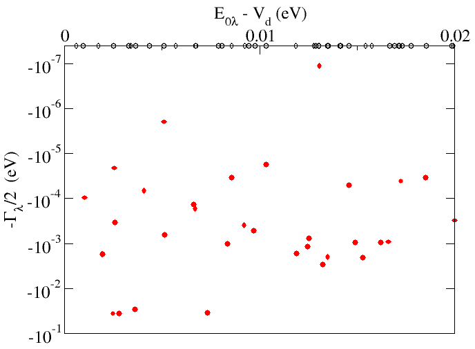
Figure 3: (Color online) Resonance energies $\bar{E}_{0\lambda}=E_{0\lambda}-i\,\Gamma_{\lambda}/2$ (red filled symbols) of the open quantum dot given in Fig. 1 with $V_{d}=0.0255124$ eV and real eigenenergies $E_{\lambda}$ (black empty symbols) of the corresponding closed dot.

As can be seen from Fig. 3, the open quantum dot strongly coupled to the source and drain contacts supports resonances with different widths, from very narrow, generally associated with modes localized within the dot region, to very wide. This phenomenon is known in the literature as resonance trapping Müller and Rotter (2009); Rotter (2009): only certain states of an open quantum system with overlapping resonances couple with the environment and their widths increase with increasing the strength of the coupling, while the other ones are more or less decoupled from the continuumMüller and Rotter (2009); Rotter (2009). As illustrated in Fig. 3, for the quantum dot considered here there exist a few resonances with a long lifetime, but the majority of the resonant states couple to the contacts. This process is controlled by the number of the conducting channels according to Refs. [Müller and Rotter, 2009; Rotter, 2009]: In the strong coupling regime $N_{1}(E)+N_{2}(E)$ resonant states couple to the environment becoming quasi-delocalized. As we have shown in Sec. II, this number is energy dependent and increases with increasing $E$. This result is physically correct because the poles of the scattering matrix having real part much higher than the scattering potential, $E\gg\max[V(x,y)]$, have also a large imaginary part irrespective of the potential landscape.

The decomposition (21) of the scattering matrix ${\tilde{\mbox{${\mathbf{\cal{S}}}$}}}$ in a resonant and a background term is especially relevant for energies inside a resonance domain. According to Eq. (21) all matrix elements of $\tilde{\cal{S}}$ and, in turn, all transmission coefficients $T_{nn^{\prime}}$ between the scattering channels have a similar dependence on energy around a resonance.

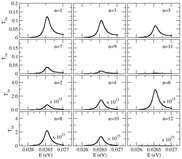
Figure 4: Transmission as a function of energy around the resonance energy $E_{0\lambda}=0.026537$ eV for the quantum dot described in Fig. 1 and $V_{d}=0.0255124$ eV.

In Fig. 4 we plot the transmission between the channel $(11)$ and the channels $(2n)$, $n\leq N_{F}$ for energies around a fixed isolated resonance. In the case of a symmetrical system the parity plays an important role. For the odd quantum number $n$ the function $\phi_{n}(y)$ has the same symmetry as $\phi_{1}(y)$, and the transmission coefficient $T_{1n}$ has a maximum around the resonance. If the parity is not conserved the transmission is forbidden, i. e., $T_{1n}\simeq 0$, $n=2,4,...$. The plots in Fig. 4 confirm the similar energy dependence of the transmission coefficients and we can conclude that a resonance can be completely characterized by the sum of these coefficients, i. e., by the total transmission. In Ref. [Nakanishi et al., 2004] a similar idea was proposed and a global Fano asymmetry parameter was defined as a linear combination of the parameters corresponding to different scattering channels.

The plot of the transmission coefficients, Fig. 4, shows a strong coupling between the scattering channels in the Fano regime of transport. The two quantum point contacts, specific for the SET geometryKastner (1992); Göres et al. (2000), control the strength of the coupling with the rest of the quantum wire and confer the scattering potential its nonseparable character responsible for the channel mixing. In this case, a resonance cannot be associated anymore with a single scattering channel as proposed in the models based on the Feshbach formalism in Refs. [Nöckel and Stone, 1995; Satanin and Joe, 2005]. The resonance perturbation theorySatanin and Joe (2005) used there to describe the coupling between the scattering channels can have limitations for large coupling strength and becomes certainly very laborious for a system with many conducting channels. In our model the 2D Schrödinger equation is directly solved combining the scattering theory with the R-matrix formalism and this method can be used to describe each coupling regime.

IV Conductance through open quantum dots

The most common method to analyze experimentally a quantum dot is to measure its conductance. In the limits of the Landauer-Büttiker formalism Büttiker et al. (1985); Büttiker (1986) and for very low temperatures, the linear conductance is given as the total transmission through the dot at the Fermi energy,

$$G(V_{d})=\frac{2e^{2}}{h}T(E_{F};V_{d}),$$ (26)

for different values of the potential energy in the dot region. Each variation of $V_{d}$ changes the scattering potential and, in turn, the total transmission.

In Figs. 5(a), 6(a), 7(a) the conductance is plotted as a function of $E_{F}-V_{d}$ for the quantum dot presented in Fig. 1 with the parameter given in Sec. III. The conductance shows peaks with line shapes from symmetric Breit-Wigner up to strong asymmetric ones and even dips or antiresonances. These maxima and minima are usually associated with resonances. Some peaks in the conductance reach values greater than 1 and that means that at least two resonances interplay to determine the line shape.

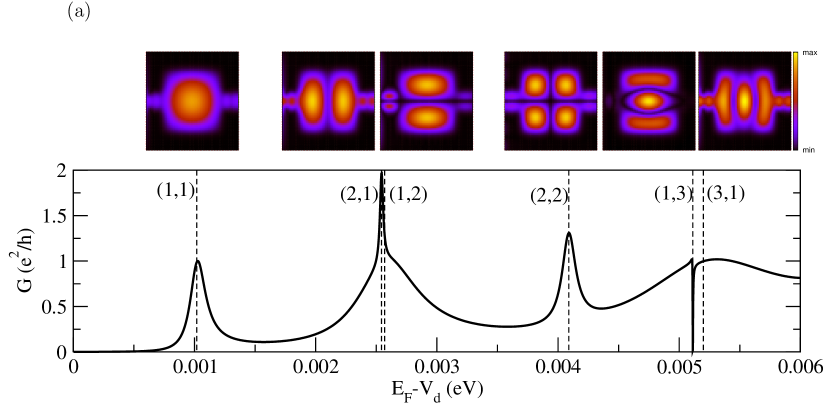
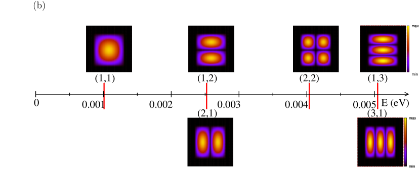
Figure 5: (Color online) (a): Conductance as a function of the potential energy in the dot region. The maps represent the electron probability distribution density inside the dot, $|\psi_{n}^{(s)}(E_{F};x,y)|^{2}$ for $V_{d}=V_{0}^{(n_{x},n_{y})}$ (vertical dashed lines) for which $E_{0}^{(n_{x},n_{y})}\simeq E_{F}$; The incident scattering channel is $n=1$ for the odd modes in the lateral direction and $n=2$ for the even ones. (b): The eigenenergies $\tilde{E}_{n_{x},n_{y}}$ and the maps of the eigenstates, $|\tilde{\psi}_{n_{x},n_{y}}(x,y)|^{2}$, for the isolated dot. Bright corresponds to high values and dark corresponds to low values.

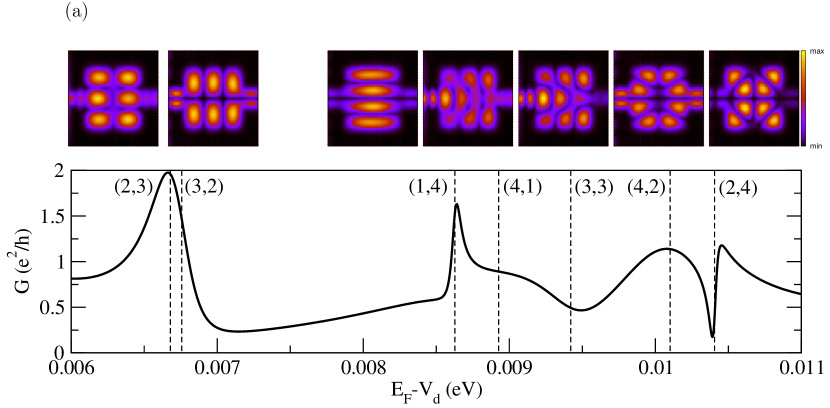
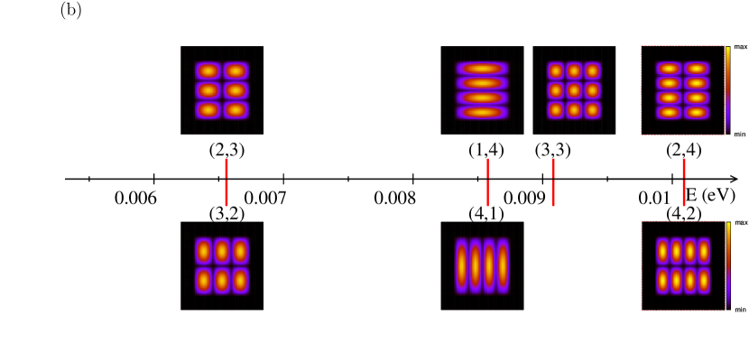
Figure 6: (Color online) (a): Conductance as a function of the potential energy in the dot region. The maps represent the electron probability distribution density inside the dot, $|\psi_{n}^{(s)}(E_{F};x,y)|^{2}$ for $V_{d}=V_{0}^{(n_{x},n_{y})}$ (vertical dashed lines) for which $E_{0}^{(n_{x},n_{y})}\simeq E_{F}$; The incident scattering channel is $n=1$ for the odd modes in the lateral direction and $n=2$ for the even ones. (b): The eigenenergies $\tilde{E}_{n_{x},n_{y}}$ and the maps of the eigenstates, $|\tilde{\psi}_{n_{x},n_{y}}(x,y)|^{2}$, for the isolated dot. Bright corresponds to high values and dark corresponds to low values.

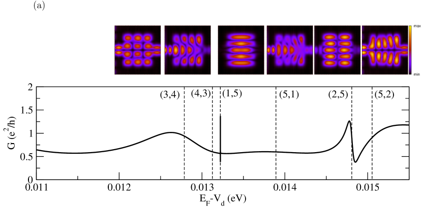
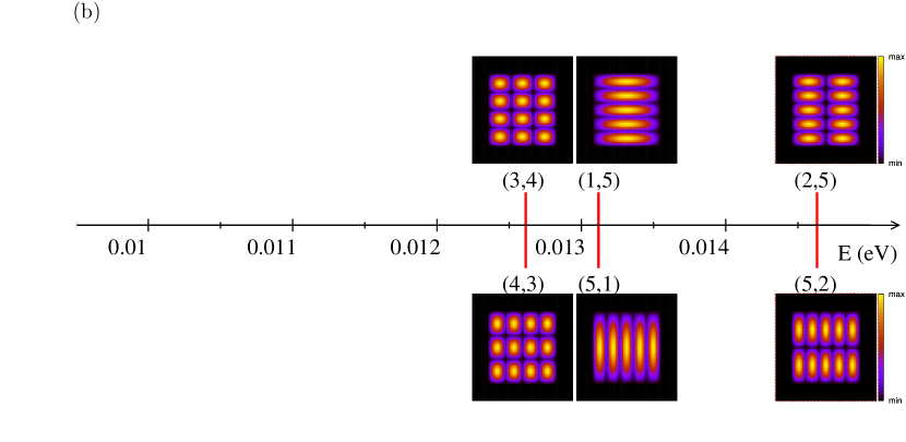
Figure 7: (Color online) (a): Conductance as a function of the potential energy in the dot region. The maps represent the electron probability distribution density inside the dot, $|\psi_{n}^{(s)}(E_{F};x,y)|^{2}$ for $V_{d}=V_{0}^{(n_{x},n_{y})}$(vertical dashed lines) for which $E_{0}^{(n_{x},n_{y})}\simeq E_{F}$; The incident scattering channel is $n=1$ for the odd modes in the lateral direction and $n=2$ for the even ones. (b): The eigenenergies $\tilde{E}_{n_{x},n_{y}}$ and the maps of the eigenstates, $|\tilde{\psi}_{n_{x},n_{y}}(x,y)|^{2}$, for the isolated dot. Bright corresponds to high values and dark corresponds to low values.

We analyze further in detail, in terms of resonances, each type of peak and dip of the conductance. For this purpose we need a functional dependence of the total transmission on $V_{d}$, at least an approximation, around the peak maximum $V_{0}$. In the case of a dip in the conductance, $V_{0}$ denotes the position of the minimum. The R-matrix formalism used for solving the scattering problem allows, in a sense, for a very intuitive approach of $T(E_{F},V_{d})$. A small variation $\delta V=V_{d}-V_{0}$ of the potential energy felt by the electron in the dot region can be approximately seen as a shift of the potential energy in the whole scattering area. In turn, the Wigner-Eisenbud energies are shifted with $\delta V$ and the Wigner-Eisenbud functions remain unchanged. For the R-matrix, Eq. (12), we can then write $\mathbf{R}(E;V_{0}+\delta V)\simeq\mathbf{R}(E-\delta V;V_{0})$. This approximation is also valid for the total transmission

$$T(E_{F};V_{0}+\delta V)\simeq T(E_{F}-\delta V;V_{0}),$$ (27)

because the wave vector $k_{sn}$ is a slowly varying energy function. A detailed discussion about this approach is given in Appendix A, Ref. [Racec and Wulf, 2001] for the open quantum dot without channel mixing.

Based on the relation (27), each peak in conductance can be associated with one or more resonances. We consider first an isolated resonance with the complex energy $\bar{E}_{0\lambda}=E_{0\lambda}-i\Gamma_{\lambda}/2$. The total transmission shows a peak around $E_{0\lambda}$ that can be also seen in conductance if $E_{0\lambda}$ matches the Fermi energy, $E_{0\lambda}=E_{F}$. Therefore, a maximum in conductance at $V_{d}=V_{0\lambda}$ corresponds to a resonance $\lambda$ and the quantity $E_{F}-V_{0\lambda}$ gives the position of the resonance energy with respect to $V_{d}$. In this way the resonance energies can be directly compared with the eigenenergies of the isolated quantum dot. In view of the experiments presented in Ref. [Göres et al., 2000], this is a square dot with the dimension $2d\times 2d$, $d=d_{x}-d_{b}$, confined by a hard wall potential as depicted in Fig. 2(b). Its eigenenergies

$$\tilde{E}_{n_{x},n_{y}}=V_{d}+\frac{\hbar^{2}}{2m^{*}}\left(\frac{\pi}{2d}\right)^{2}(n_{x}^{2}+n_{y}^{2}),\quad n_{x},\,\,n_{y}\geq 1,$$ (28)

are plotted in Figs. 5(b), 6(b), 7(b). The positions of the resonance energies are indicated by dashed lines in Figs. 5(a), 6(a), 7(a). As can be seen from these plots, the open character of the quantum system determines a shift of the eigenenergies in the complex energy plane, not only on the imaginary axis but also on the real axis. Due to the two quantum point contacts, which couple the quantum dot to the source and drain, the symmetry of the square dot is broken and the level degeneracy for $n_{x}\neq n_{y}$ is lifted.

A deep understanding of the transport properties through the open quantum dot requires a detailed analysis of the electron probability distribution density within the dot region, and the comparison of the resonance energies of the open dot with the eigenenergies of the isolated dotAkis et al. (2002). In the upper part of Figs. 5(a), 6(a), and 7(a) the functions $|\psi_{n}^{(1)}(E_{F};x,y)|^{2}$, $n=1$ or $n=2$, are given for $x$ and $y$ inside the scattering area and for $V_{d}$ corresponding to the maxima and minima in the conductance. These functions are called resonant states or resonant modes. For comparison the eigenstates $|\tilde{\psi}_{n_{x},n_{y}}(x,y)|^{2}$ of the isolated dot [see Fig. 2(b)] are presented in Figs. 5(b), 6(b), and 7(b), where

$$\tilde{\psi}_{n_{x},n_{y}}(x,y)=\frac{1}{d}\sin\left[\frac{\pi n_{x}}{2d}(x+d)\right]\sin\left[\frac{\pi n_{y}}{2d}(y+d)\right],$$ (29)

$n_{x}\geq 1$ and $n_{y}\geq 1$. The function $|\tilde{\psi}_{n_{x},n_{y}}(x,y)|^{2}$ has $n_{x}$ maxima in the $x$-direction and $n_{y}$ maxima in the $y$-direction. All modes $(n_{x},n_{y})$ that we know from the isolated dot are also found for the open dot. Some of them are strongly modified due to the coupling with the contacts, but there are also modes that do not change much. Based on the similarities of the scattering functions at the resonance energy, $|\psi_{n}^{(s)}(E_{F};x,y)|^{2}$ for $V_{d}=V_{0\lambda}$ for which $E_{0\lambda}=E_{F}$, to the eigenfunctions $|\tilde{\psi}_{n_{x},n_{y}}(x,y)|^{2}$ of the isolated dot, we associate further a pair of quantum numbers $(n_{x},n_{y})$ with each resonance $\lambda$, and the resonance energies $\bar{E}_{0\lambda}$ will be further on denoted by $\bar{E}_{0}^{(n_{x},n_{y})}=E_{0}^{(n_{x},n_{y})}-i\Gamma^{(n_{x},n_{y})}/2$. The potential energy in the dot region $V_{0\lambda}$, for which $E_{0}^{(n_{x},n_{y})}$ matches the Fermi energy, will be denoted by $V_{0}^{(n_{x},n_{y})}$. In this way the resonances are classified using a very intuitive criterion.

IV.1 Peaks associated with isolated resonances

First we analyze the slight asymmetric conductance peaks associated with an isolated resonance denoted by $\lambda$ or by $(n_{x},n_{y})$. In the energy domain of this resonance the scattering matrix $\tilde{\mbox{${\mathbf{\cal{S}}}$}}$ is given as a sum of a resonant term and a background, Eq. (21). Based on this relation and on the definition (19), the total transmission can be similarly decomposed. According to the relation (27) and for small variation $\delta V$ of the potential energy around $V_{0\lambda}$ (for which $E_{0\lambda}\simeq E_{F}$), the conductance, Eq. (26), follows the energy dependence of the transmission and becomes

$$G(V_{0\lambda}+\delta V)\simeq G_{res}(E_{F}-\delta V;V_{0\lambda})+G_{bg}(E_{F}-\delta V;V_{0\lambda}).$$ (30)

The resonant contribution to the conductance is an energy dependent function defined for each value of the potential energy in the dot region as

$$G_{res}(E;V_{d})=\frac{2e^{2}}{h}T_{0\lambda}(E)\left[\left|\frac{2i}{E-E_{\lambda}-\bar{\cal{E}}_{\lambda}(E)}-\frac{1}{\bar{q}_{\lambda}(E)}\right|^{2}-\left|\frac{1}{\bar{q}_{\lambda}(E)}\right|^{2}\right]$$ (31)

with

$$T_{0\lambda}(E)=\left|\vec{\beta}_{1\lambda}\right|^{2}\left|\vec{\beta}_{2\lambda}\right|^{2},$$ (32)

and the energy-dependent Fano asymmetry parameterMagunov et al. (2003)

$$\frac{1}{\bar{q}_{\lambda}(E)}=\frac{1}{T_{0\lambda}}\vec{\beta}_{1\lambda}^{\dagger}\mbox{\boldmath$\sigma$}_{\lambda}\vec{\beta}_{2\lambda}^{*},$$ (33)

where $(\vec{\beta}_{s\lambda})_{n}=(\vec{\beta}_{\lambda})_{sn}$, $s=1,2$ and $(\mbox{\boldmath$\sigma$}_{\lambda})_{nn^{\prime}}={\tilde{\mbox{${\mathbf{\cal{S}}}$}}}_{2n,1n^{\prime}}$, $n,n^{\prime}\geq 1$; The symbol $*$ denotes the complex conjugate. The background contribution to the conductance is given as

$$G_{bg}(E)=\frac{2e^{2}}{h}\mbox{Tr}[\mbox{\boldmath$\sigma$}_{\lambda}(E)\mbox{\boldmath$\sigma$}_{\lambda}^{\dagger}(E)].$$ (34)

The functions $G_{res}$ and $G_{bg}$ are obtained from the expression (21) of the scattering matrix without any approximation.

The first contribution to the conductance, $G_{res}$, contains a resonant term singular at $E=\bar{E}_{0\lambda}$ and a term $1/\bar{q}_{\lambda}$ that describes the coupling of the resonance $\lambda$, characterized by the vector $\vec{\beta}_{\lambda}$, to the other resonances, characterized by the background matrix $\mbox{\boldmath$\sigma$}_{\lambda}$. The function $G_{res}$ yields always a peak mainly localized in the resonance domain. Due to the coupling of the considered resonance with the other ones, this peak cannot have in principle a Breit-Wigner line shape, even in the case of a narrow and isolated resonance; The lowest approximation for a resonant peak is a Fano line shape with a complex asymmetry parameter obtained for $\bar{q}_{\lambda}(E)\simeq$ constant. The two terms add coherently to the conductance and it is usual to call $G_{res}$ the coherent part Racec and Wulf (2001). The second contribution to the conductance is the noncoherent partRacec and Wulf (2001) given only by the background matrix $\mbox{\boldmath$\sigma$}_{\lambda}(E)$. In the case of an isolated resonance $\lambda$, it is expected that $G_{bg}$ is almost constant inside the resonance domain.

The conductance curve given in Figs. 5(a), 6(a) and 7(a) shows two peaks that can be associated with isolated resonances. They correspond to the resonances (1,1) and (2,2) as follows from the analysis of the electron probability distribution density in the dot region [first and third maps in Fig. 5(a)]. For these two peaks the resonant and the background contributions to the conductance are plotted in Fig. 8. As expected, the resonant part is given by a slight asymmetric Fano line and the background is almost constant.

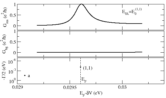
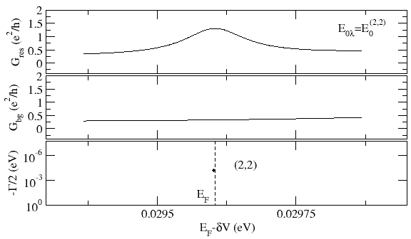
Figure 8: Conductance peaks associated with isolated resonances: (a)$(n_{x},n_{y})=(1,1)$; (b)$(n_{x},n_{y})=(2,2)$. Upper part: Resonant part of the conductance $G_{res}$; Middle part: Background part of the conductance $G_{bg}$. Lower part: Poles and position of the Fermi level in the complex energy plane. The potential energy in the dot region is constant, $V_{d}=V_{0}^{(n_{x},n_{y})}$

.

But, unexpected is the fact that the two peaks are quite wide compared to the other ones in the conductance curve. The only possible explanation is related to the presence of the quantum point contacts, which modify dramatically the scattering process and the picture which we have from the effective 1D scattering problem is no longer valid. In the case of the quantum dot studied here, the coupling between the scattering channels dominates the transmission through the dot and the scattering problem cannot be anymore reduced to a series of 1D problems. In turn, in the presence of the channel mixing the resonance widths do not increase monotonically with the energy.

As can be seen in Fig. 8, near the main resonances $(1,1)$ and $(2,2)$, there exist other ones denoted by ”$a$”. They are broader, i. e., larger imaginary part, and are associated with modes localized mainly in the region of the two quantum point contacts, as shown in Fig. 9.

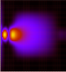
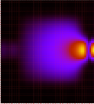
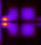
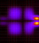
Figure 9: (Color online) Electron probability distribution densities: (a) $|\psi^{(1)}_{1}(x,y)|^{2}$ and (b) $|\psi^{(2)}_{1}(x,y)|^{2}$ for the mode associated with the resonance ”$a$” in Fig. 8(a); (c) $|\psi^{(1)}_{2}(x,y)|^{2}$, and (d) $|\psi^{(2)}_{2}(x,y)|^{2}$ for the mode associated with the resonance ”$a$” in Fig. 8(b).

The resonances of type ”$a$” do not influence directly the transmission through the open quantum dot, but they play a decisive role in the coupling process of an eigenstate to the continuum of states in the contacts. There are many modes localized in the point contact regions with the resonant energies around the Fermi energy, but only for a favorable symmetry they can intermediate a coupling between the quantum system and the source and drain contacts. The probability distribution densities given in Fig. 9 shows evidently a coupling of the modes of type ”$a$” with the resonant modes $(1,1)$ and $(2,2)$. In this case, one can speak about an interaction between the two types of resonances. In the next section we will study this phenomenon for resonances localized within the dot region, which are very close in energy and have the same symmetry in the lateral direction.

IV.2 Peaks associated with overlapping resonances

Even in the case of a simple dot geometry, there exist only a few isolated resonances. The other peaks in the conductance with strong asymmetric line shapes or maximum values about 2 are typical for the scattering processes dominated by two or more resonances, whose resonance domains cross, i. e., overlapping resonances. How strong the overlapping resonances interact is determined by their relative position in energyAkis et al. (2002) and by their symmetry in the lateral directionSatanin and Joe (2005) (perpendicular to the transport direction).

Let assume that there exists a second resonance $\lambda^{\prime}\equiv(n^{\prime}_{x},n^{\prime}_{y})$ around the Fermi energy, i. e., in the vicinity of the first resonance $\lambda\equiv(n_{x},n_{y})$, and this is a broader one, $\Gamma_{\lambda}^{\prime}>\Gamma_{\lambda}$. The presence of the second resonance leads to a strong variation of the background term $\tilde{\mbox{${\mathbf{\cal{S}}}$}}_{\lambda}$ with the energy around $E_{F}$. The expression of $\tilde{\mbox{${\mathbf{\cal{S}}}$}}_{\lambda}$, Eq. (24), similar to $\tilde{\mbox{${\mathbf{\cal{S}}}$}}$, Eq. (21), allows for a further decomposition of this term in a second resonant term and a new background. Following the method described in Sec. III, we can write

$${\tilde{\mbox{${\mathbf{\cal{S}}}$}}}_{\lambda}(E)=2iu_{0}\frac{\mathbf{\Theta}\,\vec{\beta}^{\prime}_{\lambda}\,\vec{\beta}^{\prime\,T}_{\lambda}\,\mathbf{\Theta}}{E-E_{\lambda^{\prime}}-\bar{\cal{E}}_{\lambda}^{\prime}}+{\tilde{\mbox{${\mathbf{\cal{S}}}$}}^{\prime}}_{\lambda}(E),$$ (35)

where $\vec{\beta}^{\prime}_{\lambda}$, $\bar{\cal{E}}_{\lambda}^{\prime}(E)$, and ${\tilde{\mbox{${\mathbf{\cal{S}}}$}}^{\prime}}_{\lambda}$ can be obtained from $\vec{\beta}_{\lambda}$, $\bar{\cal{E}}_{\lambda}(E)$, and ${\tilde{\mbox{${\mathbf{\cal{S}}}$}}}_{\lambda}$, Eqs. (22), (23), and (24), respectively, by replacing $\vec{\alpha}_{\lambda}$ by $\vec{\alpha}_{\lambda^{\prime}}$ and $\mathbf{\Omega}_{\lambda}$ by $\mathbf{\Omega}^{\prime}_{\lambda}=\mathbf{\Omega}_{\lambda}-u_{0}\frac{\vec{\alpha}_{\lambda^{\prime}}\,\vec{\alpha}^{T}_{\lambda^{\prime}}}{E-E_{\lambda^{\prime}}}$. Thus, the background contribution of the first resonance to the conductance, Eq. (34), becomes a sum of two contributions,

$$G_{bg}(E_{F};V_{d})=G^{\prime}_{res}(E_{F};V_{d})+G^{\prime}_{bg}(E_{F};V_{d}),$$ (36)

a resonant one,

$$G^{\prime}_{res}(E;V_{d})=\frac{2e^{2}}{h}T^{\prime}_{0\lambda}(E)\left[\left|\frac{2i}{E-E_{\lambda^{\prime}}-\bar{\cal{E}}^{\prime}_{\lambda}(E)}-\frac{1}{\bar{q}^{\prime}_{\lambda}(E)}\right|^{2}-\left|\frac{1}{\bar{q}^{\prime}_{\lambda}(E)}\right|^{2}\right]$$ (37)

with a similar energy dependence as $G_{res}(E;V_{d})$ and a second background,

$$G^{\prime}_{bg}(E;V_{d})=\frac{2e^{2}}{h}\mbox{Tr}[\mbox{\boldmath$\sigma$}_{\lambda}^{\prime}(E)\mbox{\boldmath$\sigma$}_{\lambda}^{\prime\dagger}(E)]$$ (38)

with $(\mbox{\boldmath$\sigma$}^{\prime}_{\lambda})_{nn^{\prime}}={\tilde{\mbox{${\mathbf{\cal{S}}}$}}}^{\prime}_{2n,1n^{\prime}}$, $n,n^{\prime}\geq 1$, slowly varying with the energy if a third resonance does not exist around $E_{F}$. The energy-dependent Fano asymmetry parameter $\bar{q}^{\prime}_{\lambda}(E)$ in Eq. (37), associated with the resonance $\lambda^{\prime}$, has the expression

$$\frac{1}{\bar{q}^{\prime}_{\lambda}(E)}=\frac{1}{T^{\prime}_{0\lambda}}\vec{\beta}_{1\lambda}^{{}^{\prime}\dagger}\mbox{\boldmath$\sigma$}^{\prime}_{\lambda}\vec{\beta}_{2\lambda}^{{}^{\prime}*},$$ (39)

where $T^{\prime}_{0\lambda}(E)=\left|\vec{\beta}^{\prime}_{1\lambda}\right|^{2}\left|\vec{\beta}^{\prime}_{2\lambda}\right|^{2}$ and $(\vec{\beta}^{\prime}_{s\lambda})_{n}=(\vec{\beta}^{\prime}_{\lambda})_{sn}$, $s=1,2$, $n\geq 1$. The expression (36) is also exact and we have only rearranged the terms in order to put directly in evidence the contributions of each resonance to the conductance. The second background term, $G^{\prime}_{bg}$, gives the possibility of a further decomposition in a third resonant term and a new background in the case of three interacting resonances around the Fermi energy.

For a systematic mathematical calculation we have also to consider the energy dependence of $\mbox{\boldmath$\sigma$}_{\lambda}$, Eq. (35), in the expression (33) of the Fano asymmetry parameter associated with the first resonance,

$$\frac{1}{\bar{q}_{\lambda}}=\frac{1}{T_{0\lambda}}\left[\vec{\beta}_{1\lambda}^{\dagger}\mbox{\boldmath$\sigma$}^{\prime}_{\lambda}\vec{\beta}_{2\lambda}^{*}+2iu_{0}\frac{\vec{\beta}_{1\lambda}^{\dagger}\cdot\vec{\beta}_{1\lambda}^{\prime}\,\vec{\beta}_{2\lambda}^{\dagger}\cdot\vec{\beta}_{2\lambda}^{\prime}}{E-E_{\lambda^{\prime}}-\bar{\cal{E}}_{\lambda}^{\prime}}\right].$$ (40)

The function $1/{\bar{q}_{\lambda}}$ is responsible for the asymmetry of the resonant contribution $G_{res}$, Eq. (31), that has a singularity at $\bar{E}=\bar{E}_{0\lambda}$. The presence of a second resonance $\lambda^{\prime}$ around $\lambda$ yields in $1/{\bar{q}_{\lambda}}$ a term singular at $\bar{E}=\bar{E}_{0\lambda^{\prime}}$.

If the first resonance is very narrow and the second one broaden, $\Gamma_{\lambda}\ll\Gamma_{\lambda^{\prime}}$, the Fano asymmetry parameter $1/{\bar{q}_{\lambda}}$ varies slowly with the energy compared to the term in $G_{res}$ singular at $\bar{E}=\bar{E}_{0\lambda}$. In this case, the energy dependence of $1/{\bar{q}_{\lambda}}$ can be neglected around the resonance $\lambda$ and an energy-independent Fano asymmetry parameter can be defined. These results are in agreement with Ref. [Magunov et al., 2003]. The resonant contribution to the conductance is then given as a Fano functionFano and Rau (1986) $f(e)=|e+\bar{q}_{F}|^{2}/(e^{2}+1)$ with a complex asymmetry parameter $\bar{q}_{F}$. For $|1/\bar{q}_{F}|\ll 1$ this function has a quasi Breit-Wigner profile, while for $|1/\bar{q}_{F}|\gg 1$ it becomes a symmetric dip, usually called antiresonance. The intermediate values $|1/\bar{q}_{F}|\simeq 1$ correspond to a Fano function characterized by a maximum and a minimum approximatively equidistant to the axis $e=1$ and we call this profile a ”S-type” Fano line. For open quantum dots, the different Fano profiles can be associated with different types of interacting resonances. From Eq. (40) it follows that $\bar{q}_{\lambda}\sim\vec{\beta}_{\lambda}\cdot\vec{\beta}^{\prime}_{\lambda}$ for a second resonance much broader than the first one. The two vectors $\vec{\beta}_{\lambda}$ and $\vec{\beta}^{\prime}_{\lambda}$, characterize the two considered resonances, and their scalar product is in principle nonzero. If the two resonant modes have different parities in the lateral direction, the vectors $\vec{\beta}_{\lambda}$ and $\vec{\beta}^{\prime}_{\lambda}$ are approximatively orthogonal to each other and, in turn, the Fano asymmetry parameter has values from small to intermediate. In this case, we can speak about a weak interaction between the overlapping resonances. In contrast, for the same parity in the lateral direction, the vectors $\vec{\beta}_{\lambda}$ and $\vec{\beta}^{\prime}_{\lambda}$ are approximatively parallel to each other and the Fano asymmetry parameter corresponds to a dip. In this case, the two overlapping resonances interact strongly. In Ref. [Satanin and Joe, 2005] the antiresonances in the conductance through two identical quantum dots embedded in a wave guide were also related to strong interacting resonances with the same parity.

In the case of two overlapping resonances with comparable widths, both the term in $G_{res}$ singular at $\bar{E}=\bar{E}_{0\lambda}$ and the Fano asymmetry parameter (40) vary slowly with the energy and we can not predict the line shape around the resonances. This situation corresponds to a wide peak in the conductance.

Summarizing all the above results and using the approximative expression of the total transmission around a resonance at the Fermi energy, Eq. (27), we obtain for the conductance

$$G(V_{0\lambda}+\delta V)\simeq G_{res}(E_{F}-\delta V;V_{0\lambda})+G_{res}^{\prime}(E_{F}-\delta V;V_{0\lambda})+G_{bg}^{\prime}(E_{F}-\delta V;V_{0\lambda}),$$ (41)

where $V_{0}^{(n_{x},n_{y})}=V_{0\lambda}$ is the potential energy in the dot region for which the resonance with the longest life-time ($\Gamma_{\lambda}<\Gamma_{\lambda^{\prime}}$) matches the Fermi energy. Based on the above relation, we identify the contribution of each resonance to the conductance and distinguish between weak and strong coupling regime of two overlapping resonances. The information about the strength of the coupling between the resonances $\lambda\equiv(n_{x},n_{y})$ and $\lambda^{\prime}\equiv(n^{\prime}_{x},n^{\prime}_{y})$ is contained into the energy-dependent Fano asymmetry parameter, Eq. (33), and it determines the line shape of the resonant contribution $G_{res}$ to the conductance. The other two components of the conductance, $G^{\prime}_{res}$ and $G^{\prime}_{bg}$, provide information about the interaction of the second resonance $(n^{\prime}_{x},n^{\prime}_{y})$ with all other resonances of the system excepting the two already considered. A strong variation with the energy of the function $G^{\prime}_{bg}$ in the energy domain of the resonance $(n^{\prime}_{x},n^{\prime}_{y})$ indicates the presence of a third resonance $(n^{\prime\prime}_{x},n^{\prime\prime}_{y})$ around the Fermi energy. From the line shape of the resonant component $G^{\prime}_{res}$ we can, in principle, get the information about how strong this third resonance interacts with the resonance $(n^{\prime}_{x},n^{\prime}_{y})$.

IV.2.1 Weak interacting resonances

In the weak interaction regime the two overlapping resonances are close in energy but they do not perturb each other significantly. Each of them contributes to the conductance as a quasi-isolated resonance and the line shape of the peak is given as a superposition of two Fano lines with a slight up to an intermediate asymmetry. This is the case of the second peak in Fig. 5(a) and the first peak in Fig. 6(a), for which the different contributions to the conductance are analyzed in detail in Fig. 10. The two peaks correspond to the pair of resonances $(1,2)$ and $(2,1)$ and $(2,3)$ and $(3,2)$.

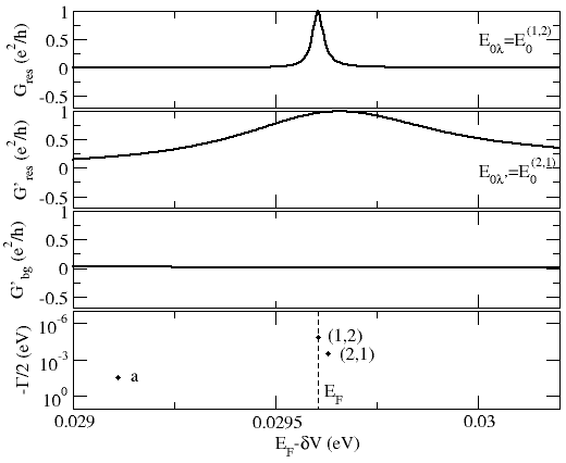
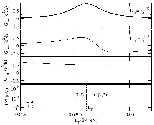
Figure 10: Conductance peaks associated with isolated resonances: (a)$\lambda=(1,2)$, $\lambda^{\prime}=(2,1)$; (b)$\lambda=(2,3)$, $\lambda^{\prime}=(3,2)$. Upper parts: Resonant parts of the conductance $G_{res}$ and $G^{\prime}_{res}$ and background part $G^{\prime}_{bg}$; Lower part: Poles and position of the Fermi level in the complex energy plane. The potential energy in the dot region is constant, $V_{d}=V_{0\lambda}$.

In both situations the overlapping resonances have at the origin a degenerate eigenstate of the isolated dot presented in Fig. 2(b), with different symmetries in the $x$- and $y$-direction. The two quantum point contacts ($V_{b1}$ and $V_{b2}$) of the open dot create a strong coupling regime to the conducting leads and break the square symmetry of the isolated dot. In turn, the degeneracy is lifted when the quantum dot becomes open and, with increasing the coupling strength, the degenerate energy level evolves into two resonances that repulse each other in the complex energy plane. This phenomenon is illustrated in the lower part of Fig. 10. The first case corresponds to the resonance trappingMüller and Rotter (2009); Rotter (2009) and the second one to the level repulsionMüller and Rotter (2009); Rotter (2009). Due to the trapping, the resonance $(1,2)$ has a longer life-time and a resonant state almost localized inside the dot region, while the resonance $(2,1)$ has a shorter life-time and shows a significant probability distribution density in the region of the two quantum point contacts. The state with the nearest maximum to the aperture couples stronger to the contacts and yields a broader contribution to the conductance compared to the first resonance. Both of them are described by Fano lines with a slight asymmetry corresponding to a weak interaction between the overlapping resonances and with the background. Figure 10(b) shows the resonances $(2,3)$ and $(3,2)$, which have comparable widths and are well separated in energy. From the probability distribution density of these two modes, Fig. 6(a), it is evident that both of them can easy couple to the modes localized in the point contact regions, modes denoted by ”$a$” and presented in Fig. 9. In this case, the resonance trapping is not favorable. The both resonant modes couple to the contacts via two modes of type ”$a$”. The line shape of $G_{res}$ corresponds to a weak interaction between the resonances $(2,3)$ and $(3,2)$, but $G^{\prime}_{res}$ indicates a stronger interaction of the second resonance with the background. The total contribution to the conductance yields in each situation a peak with a maximum about 2.

In conclusion, the weak coupling regime between overlapping resonances is characterized by probability distribution densities within the dot region similar to the eigenstates of the isolated dot. According to this rule, the resonances (1,4) and (4,1) and (3,4) and (4,3) are also weak coupled with each other, but, as we will see in the next section, in each case there is a strong coupling with another neighbor resonance which modifies the probability distribution density of the states (4,1) and (4,3), respectively. The last peak in Fig. 7(a) corresponds to the resonances $(2,5)$ and $(5,2)$ that interact also weakly and have a similar behavior to the pair $(2,3)$ and $(3,2)$.

IV.2.2 Strong interacting resonances. Hybrid modes

The really new physics of the scattering process can be seen in the case of a strong interaction between the overlapping resonances, phenomenon that does not occur in the case of an effective 1D quantum dot Racec and Wulf (2001). This coupling regime is responsible for the thin or strong asymmetric peaks and dips in the conductance and for the resonant states whose probability distribution densities differ strongly from the corresponding eigenstates of the isolated dot. Particularly for the SET geometry, Fig. 1, the strong coupling of the quantum dot to the environment is always accompanied by a strong scattering between the energy channels. This supplementary scattering determines the reordering process of the resonances in the complex energy plane, i. e., the interaction between overlapping resonances. The channel mixing influences especially the eigenstates with the same symmetry in the lateral direction. Due to the favorable parity, these modes couple with each other and generate new resonant modes that can not be supported by the isolated dot. As seen in Figs. 5, 6, and 7, there are two categories of strong coupled resonances: The first ones are the resonances that correspond to eigenstates with the same symmetry in the $x-$ and $y-$direction and whose resonant states are hybrid modes, similar to the hybrid orbitals of the natural atoms. The resonances (1,3) and (3,1), (2,4) and (4,2), and (1,5) and (5,1) belong to this category. The second category includes resonances corresponding to eigenstates with the same symmetry only in the lateral direction ($y$-direction) like the pairs (4,1) and (3,3) and (4,3) and (5,1). We associate these resonances with a strong interaction because the probability distribution densities for the states (4,1) and (5,1) are drastically modified in comparison with the isolated case.

The modes associated with strong interacting resonances yield dips or ”S-type” Fano lines in the conductance, superposed on the top of broad peaks, as shown in Figs. 5(a), 6(a), and 7(a). The overlapping resonance pairs $(1,3)$ and $(3,1)$ and $(2,4)$ and $(4,2)$ are analyzed in detail in Fig. 11. The strong interaction of these resonances, reflected by the dips in $G_{res}$, has as an effect their strong repulsion in the complex energy plane. In turn, the resonant modes $(1,3)$ and $(2,4)$ become long-lived and are practically localized within the dot region, while the modes $(3,1)$ and $(4,2)$ couple stronger to the contacts and have shorter life-time. The electron distribution in the dot region favors in the first case, Fig. 11(a), a typical resonance trapping, while in the second case, Fig. 11(b), this phenomenon is not so pronounced, but it is accompanied by a level repulsion on the real axis. The contribution of the second resonance to the conductance $G^{\prime}_{res}$ is described by a broad peak and the background $G^{\prime}_{bg}$ is almost constant.

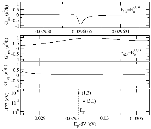
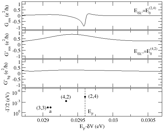
Figure 11: Conductance peaks associated with isolated resonances: (a) $\lambda=(1,3)$, $\lambda^{\prime}=(3,1)$; (b) $\lambda=(2,4)$, $\lambda^{\prime}=(4,2)$. Upper parts: Resonant parts of the conductance $G_{res}$ and $G^{\prime}_{res}$ and background part $G^{\prime}_{bg}$; Lower part: Poles and position of the Fermi level in the complex energy plane. The potential energy in the dot region is constant, $V_{d}=V_{0\lambda}$

Each pair of strong interacting resonances analyzed above corresponds to a degenerate energy level of the isolated dot and their probability distribution densities are practically linear combinations of the two eigenfunctions of the degenerate level. This property can be easy seen in Fig. 6(a) for the resonances $(2,4)$ and $(4,2)$. We can speak in this case about hybrid resonant modes. The open quantum dot behaves like the oxygen atom in the water molecule: due to the interaction with the hydrogen atoms, the $s$ and $p$ orbitals of the oxygen are mixed to new hybrid orbitals so that the total energy of the molecule is minimal. Similar, the coupling of the quantum dot to the contacts by means of two quantum point contacts yields a supplementary scattering potential which allows for new resonant modes. They are not states which survive the coupling process to the contacts Akis et al. (2002), but rather new hybrid states, whose existence is directly connected to the presence of the strong coupling regime. These modes offer the possibility of engineering quantum systems with complex properties. Even in the case of a non-perfect square quantum dot the above results remain valid. A small difference between $d_{x}$ and $d_{y}$ yields instead of a degenerate level two very close eigenvalues. Essential for the strong interaction of the two corresponding resonances is the same parity of the resonant states on both directions and not the initial degeneracy.

The resonances $(1,5)$ and $(5,1)$ interact also strongly. They determine in the conductance a very thin ”S-type” Fano line superposed onto an extreme broad peak as shown in Fig. 12(b).

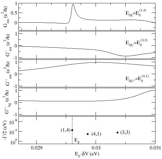
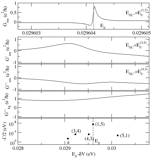
Figure 12: Conductance peaks associated with isolated resonances: (a) $\lambda=(1,4)$, $\lambda^{\prime}=(3,3)$, $\lambda^{\prime\prime}=(4,1)$; (b) $\lambda=(1,5)$, $\lambda^{\prime}=(3,4)$, $\lambda^{\prime\prime}=(4,3)$. Upper parts: Resonant parts of the conductance $G_{res}$, $G^{\prime}_{res}$, and $G^{\prime\prime}_{res}$ and background part $G^{\prime\prime}_{bg}$; Lower part: Poles and position of the Fermi level in the complex energy plane. The potential energy in the dot region is constant, $V_{d}=V_{0\lambda}$.

Their stronger repulsion in the complex energy plane compared to the precedent cases (Fig. 11) is determined by a supplemental strong interaction of the resonances $(5,1)$ and $(4,3)$, which have the same parity in the lateral direction. The maps of the probability distribution densities for the two modes in Fig. 7(a) confirm also the phenomenon of hybridization. The resonant modes $(4,3)$ and $(5,1)$ do not show such a high symmetry as the modes $(2,4)$ and $(4,2)$, but it is evident that they can be obtained as a linear combination of the eigenfunctions $(4,3)$ and $(5,1)$ of the isolated dot and the mode $(4,3)$ dominates this combination. The multiple interactions between neighbor resonances with the same symmetry in the lateral direction amplify the phenomenon of resonance trapping. One resonance - in this case resonance $(1,5)$ - decouples from the contacts and becomes extreme long-lived, while the other two become broaden and show a significant separation in energy. If we consider the quantum dot as an artificial atom it is easy to accept the hybridization as a natural process determined by the interaction with another system, but the existence of very narrow resonances supported by an open quantum dot seems to be a paradox: it is necessary to open a quantum dot, i. e., to allow for regions where the direct electron transfer between dot and contacts is possible, in order to obtain strongly localized states. Hence, long-lived modes of a quantum system can be obtained either in a quasi-isolated quantum dot or in a dot confined by shallow barriers engineered in such a way that the scattering channels are strongly mixed. The two types of localized modes have different fingerprints in the conductance: in the first case they yield quasi-symmetric maxima, while in the second case strong asymmetric Fano lines appear on top of broad peaks.

The last sequence to be discussed corresponds to the resonances $(1,4)$, $(4,1)$, and $(3,3)$ in Fig. 6(a). As can be seen from the probability distribution density maps in Fig. 6(a), there are three interacting resonances with different coupling strengths; (1,4) and (4,1) interact weakly and yield two slight asymmetric maxima in the conductance, one of them quite thin and the other one broad, Fig. 12(a). In contrast, the resonances (4,1) and (3,3) interact strongly and the resonant contribution of $(3,3)$ is a broad dip. The three interacting resonances $(4,1)$, $(3,3)$ and $(1,4)$ are very interesting in view of the experiments presented in Ref. [Göres et al., 2000]. Their contribution to the conductance together with the next peak determined by the resonances $(2,4)$ and $(4,2)$, Fig. 6(a), approximate qualitatively very well the conductance curve given in Ref. [Göres et al., 2000], Fig. 2(a), for the quantum dot in the Fano regime. Based on our resonance analysis we can conclude that the first thin peak in the measured conductance curve is superimposed on the top of a second broad peak and they correspond to two weak interacting resonances with different symmetries in the lateral direction. The next dip in the conductance reflects the presence of a resonance of type $(n,n)$ that interacts strongly with only one of the neighbor resonances. The following ”S-type” Fano line is again superimposed on a broad peak and indicates the presence of two strong interacting resonances with the same symmetry in the lateral and transport directions. For a quantitative analysis of the conductance we have to determine from the charge analysis within the dot region the value interval of $V_{d}$ that corresponds to the number of electrons found experimentallyGöres et al. (2000).

V Conclusions

We have provided in this paper a systematic treatment of the conductance through a quantum dot strongly coupled to wide conducting leads via short quantum point contacts. The electronic transport through this type of dots is essentially a scattering process in a low confining potential, which requires a direct solution of the two-dimensional Schrödinger equation with a nonseparable scattering potential. For this purpose, we have used a generalized scattering theory that allows for a complete description inside and outside the scattering area and is based on the R-matrix formalism. The resonances are determined as poles of the multidimensional scattering matrix, which contains the information about channel mixing due to the nonseparable scattering potential. The strong coupling of the quantum dot to the environment yields overlapping resonances, which show a significant interaction with each other in the case of a favorable parity of the corresponding resonant states.

The conductance is determined as a function of the potential energy within the dot region, and every peak in conductance is associated with a resonance or a group of overlapping resonances. Based on the representation of the scattering matrix in terms of the R-matrix we provide for each peak an exact decomposition of the conductance in resonant terms associated with each of the overlapping resonances and a background. The decomposition is hierarchical, i. e., from the strongest to the broadest resonance, and allows for a deep understanding of the phenomena, which determine the transmission in the case of interacting resonances. The resonant states characterizing the open quantum dot in the Fano regime are presented in comparison with the eigenstates of the isolated dot. Every resonant state has a correspondent between these eigenstates and, we distinguish between slight and strong modified states due to the coupling with the environment. The last ones are called hybrid resonant modes, and they occur only in the case of a strong coupling regime of the quantum dot to the contacts, as an effect of the interaction between resonances with the same parity. The phenomenon of hybridization evidenced here for the quantum dots in the Fano regime of transport attests the molecule-like behavior of this system and opens the possibility to realize artificial molecules based on semiconductor nanostructures.

The conductance through the quantum dot in the Fano regime of transport is also compared qualitatively to the experimental data reported in Ref. [Göres et al., 2000].

Appendix A Poles of the $\tilde{\cal{S}}$-matrix

The starting point for our pole analysis is the expression of the non-constant part in the $\tilde{\cal{S}}$-matrix in terms of $\mathbf{A}_{\lambda}=\vec{\alpha}_{\lambda}\vec{\beta}^{T}_{\lambda}/(E-E_{\lambda})$ and $\mathbf{\Omega}_{\lambda}$:

$$\mathbf{1}+i\mathbf{\Omega}=\left(\mathbf{1}+i\mathbf{A}_{\lambda}\right)\left(\mathbf{1}+i\mathbf{\Omega}_{\lambda}\right).$$ (42)

Using the definition of $\vec{\beta}_{\lambda}$, Eq. (22), we can immediately demonstrate that each determinant of the second order of $\mathbf{A}_{\lambda}$ is zero, $(\mathbf{A}_{\lambda})_{ij}(\mathbf{A}_{\lambda})_{lp}-(\mathbf{A}_{\lambda})_{ip}(\mathbf{A}_{\lambda})_{lj}=0$, where each index $i,j,l,p$ is a composite index $(sn)$ with $s=1,2$, $n\geq 1$. Therefore, the matrix $\mathbf{A}_{\lambda}$ has the rank 1. On this basis we find that

$$\mbox{det}\left[\mathbf{1}+i\mathbf{A}_{\lambda}\right]=1+i\mbox{Tr}[\mathbf{A}_{\lambda}].$$ (43)

In order to demonstrate the above relation we consider a $M\times M$ matrix $\mathbf{A}$, $M\geq 2$, with $\mbox{Rank}[\mathbf{A}]=1$, calculate the determinant of $\mathbf{1}+\mathbf{A}$ and take after that the limit $M\rightarrow\infty$. According to the definition, the determinant is given as a sum over all permutations $\pi$ of the numbers $\{1,...,M\}$

$$\mbox{det}\left[\mathbf{1}+\mathbf{A}\right] = \sum_{\pi_{M}}\mbox{sgn}\pi_{M}(\delta_{1m_{1}}+A_{1m_{1}})....(\delta_{Mm_{M}}+A_{Mm_{M}}),$$ (44)

with $m_{1},...,m_{M}\in\{1,...,M\}$, $m_{i}\neq m_{j}$ for $i\neq j$, $i,j\in\{1,...,M\}$ and $\mbox{sgn}\pi_{M}$ denotes the signature of the permutation $\pi$ and $\delta_{ij}$ is the Kronecker delta. After a direct calculation we obtain

$$\mbox{det}\left[\mathbf{1}+\mathbf{A}\right] = \;\;\;\sum_{\pi_{M}}\mbox{sgn}\pi_{M}\delta_{1m_{1}}....\delta_{Mm_{M}}$$ (47)

$$+\sum_{\pi_{M}}\mbox{sgn}\pi_{M}\delta_{1m_{1}}....\delta_{M-1m_{M-1}}A_{Mm_{M}}$$

$$+........$$

$$+\sum_{\pi_{M}}\mbox{sgn}\pi_{M}A_{1m_{1}}\delta_{2m_{2}}....\delta_{Mm_{M}}$$

$$+\sum_{\pi_{M}}\mbox{sgn}\pi_{M}\delta_{1m_{1}}....\delta_{M-2m_{M-2}}A_{M-1m_{M-1}}A_{Mm_{M}}$$

$$+........$$

$$+\sum_{\pi_{M}}\mbox{sgn}\pi_{M}A_{1m_{1}}....A_{Mm_{M}}$$

$$= 1+A_{MM}+...+A_{11}+\left|\begin{array}[]{cc}A_{M-1M-1}&A_{M-1M}\\ A_{MM-1}&A_{MM}\end{array}\right|+....+\mbox{det}[\mathbf{A}].$$

Thus, $\mbox{det}\left[\mathbf{1}+\mathbf{A}\right]$ is given as 1 plus a sum of determinants of different order of $\mathbf{A}$. But $\mbox{Rank}[\mathbf{A}]=1$ and consequently all the determinants of $\mathbf{A}$ up to the second order are zero. So that we find

$$\mbox{det}\left[\mathbf{1}+\mathbf{A}\right]=1+\mbox{Tr}[\mathbf{A}].$$ (48)

This result does not depend explicitly on the matrix dimension $M$ so that we can generalize it for the case $M\rightarrow\infty$ and obtain Eq. (43).

In the next step we calculate the adjugate matrix of $\mathbf{1}+\mathbf{A}$, i. e., $\overline{\mathbf{1}+\mathbf{A}}$, in order to invert it:

$$(\mathbf{1}+\mathbf{A})^{-1}=\frac{1}{\det[1+\mathbf{A}]}\overline{\mathbf{1}+\mathbf{A}}.$$ (49)

For a given pair of indices $ij$ the corresponding matrix element of $\overline{\mathbf{1}+\mathbf{A}}$ is calculated as the product between $(-1)^{i+j}$ and the minor $ij$ of $(\mathbf{1}+\mathbf{A})^{T}$ (the determinant of the matrix obtained from $(\mathbf{1}+\mathbf{A})^{T}$ by removing the row $i$ and the column $j$, where $T$ denotes the matrix transpose). Thus, for $i=j$ we obtain

$$(\overline{\mathbf{1}+\mathbf{A}})_{ii}=\mbox{det}[\mathbf{1}+\mathbf{B}_{ii}],$$ (50)

where $\mathbf{B}_{ii}$ is obtained from $\mathbf{A}^{T}$ by removing the row $i$ and the column $i$. The matrix $\mathbf{B}_{ii}$ is a $(M-1)\times(M-1)$ matrix with the rank 1 and therefore

$$(\overline{\mathbf{1}+\mathbf{A}})_{ii}=1+\mbox{Tr}[\mathbf{B}_{ii}]=1+\sum_{j=1}^{M-1}(\mathbf{B}_{ii})_{jj}=1+\mbox{Tr}[\mathbf{A}]-A_{ii}.$$ (51)

In the case $j=i+1$ we find

$${\overline{(\mathbf{1}+\mathbf{A})}}_{ii+1}=-\mbox{det}[\mathbf{I}_{i}+\mathbf{B}_{ii+1}],$$ (52)

where $(M-1)\times(M-1)$ matrix $\mathbf{I}_{i}$ is obtained from the unity matrix by changing 1 on the position $ii$ with 0, ($i<M$) and $\mathbf{B}_{ii+1}$ is the matrix obtained from $\mathbf{A}$ by removing the $i$-th row and the $(i+1)$-th column. This is a $(M-1)\times(M-1)$ matrix and has the rank 1. The matrix element $ii$ of $\mathbf{B}_{ii+1}$ is $A_{ii+1}$. Further we write explicitly the determinant as a sum over all permutation of the numbers $\{1,...,M-1\}$,

$$\mbox{det}[\mathbf{I}_{i}+\mathbf{B}_{ii+1}] = \sum_{\pi_{M-1}}\mbox{sgn}\pi_{M-1}(\delta_{1m_{1}}+b_{1m_{1}})....(\delta_{i-1m_{i-1}}+b_{i-1m_{i-1}})b_{im_{i}}$$ (53)

$$\qquad\qquad\qquad\times(\delta_{i+1m_{i+1}}+b_{i+1m_{i+1}})....(\delta_{M-1m_{M-1}}+b_{M-1m_{M-1}}),$$

where $b_{jl}$, with $j,l=\overline{1,M-1}$, means the matrix element $jl$ of $\mathbf{B}_{ii+1}$. Replacing $b_{im_{i}}$ by $\delta_{im_{i}}+b_{im_{i}}-\delta_{im_{i}}$ allows us to express $\overline{(\mathbf{1}+\mathbf{A})}_{ii+1}$ as $\mbox{det}[\mathbf{1}+\mathbf{B}_{ii+1}]$ minus the minor $ii$ of $\mathbf{I}_{i}+\mathbf{B}_{ii+1}$. The last two determinants can be calculated using Eq. (43) because the corresponding matrices are a sum of the unity matrix and a part of $A$-matrix which has the property $\mbox{Rank}[\mathbf{A}]=1$. Thus, we find

$$\mbox{det}[\mathbf{I}_{i}+\mathbf{B}_{ii+1}]=1+\sum_{j=1}^{M-1}b_{jj}-\left[1+\sum_{j=1}^{i-1}b_{jj}+\sum_{j=i+1}^{M-1}b_{jj}\right]$$ (54)

and after that, using Eq. (48),

$${\overline{(\mathbf{1}+\mathbf{A})}}_{ii+1}=-A_{ii+1}.$$ (55)

Further we analyze the case $j>i+1$. If we eliminate the $i$-th row and the $j$-th column in $(\mathbf{1}+\mathbf{A})^{T}$ we obtain a matrix which does not have any more elements of the type $1+a_{ll}$ on the main diagonal between the column $i$ and $j-1$. These elements are on the positions $l-1l$, $l=\overline{i+1,j-2}$. Taking into account that we only need to calculate the determinant of this matrix we exchange the columns: $i\leftrightarrow i+1$, …, $j-2\leftrightarrow j-1$ and each of these $j-i-1$ operations changes the determinant with -1. So that we can write

$${\overline{(\mathbf{1}+\mathbf{A})}}_{ij}=(-1)^{i+j+j-i-1}\mbox{det}[\mathbf{I}_{j-1}+\mathbf{B}_{ij}].$$ (56)

As described above the matrix $\mathbf{B}_{ij}$ is obtained from $\mathbf{A}^{T}$ by removing the $i$-th row and the $j$-th column and after that by exchanging the columns $i\leftrightarrow i+1$, …, $j-2\leftrightarrow j-1$. This $(M-1)\times(M-1)$ matrix has also rank 1 and the matrix element $j-1j-1$ of $\mathbf{B}_{ij}$ is $A_{ij}$, i. e., $\left(\mathbf{B}_{ij}\right)_{j-1j-1}=A_{ij}$. Similar to the previous case we can demonstrate here that

$${\overline{(\mathbf{1}+\mathbf{A})}}_{ij}=-A_{ij}.$$ (57)

With the same procedure we can demonstrate that the above result remains also valid for $j<i$.

If we put together the main results of this section, Eqs. (43), (51), (55), and (57), we find

$$(\mathbf{1}+\mathbf{A})^{-1}=\mathbf{1}-\frac{\mathbf{A}}{1+\mbox{Tr}[\mathbf{A}]}.$$ (58)

The above relation does not depend essentially on $M$, so that we can take the limit $M\rightarrow\infty$ and generalize Eq. (58) for $i\mathbf{A}_{\lambda}$. After that we obtain from Eq. (42) that

$$(\mathbf{1}+i\mathbf{\Omega})^{-1}=(\mathbf{1}+i\mathbf{\Omega}_{\lambda})^{-1}\left(\mathbf{1}-\frac{i\mathbf{A}_{\lambda}}{1+i\mbox{Tr}[\mathbf{A}_{\lambda}]}\right).$$ (59)

Feeding this relation into the definition of $\tilde{\cal{S}}$-matrix, Eq. (15), we find Eq. (21).

References

- Ferry and Goodnick (1997) D. K. Ferry and S. M. Goodnick, Transport in Nanostructures (Cambridge University Press, Cambridge, 1997).
- Nazarov and Blanter (2009) Y. V. Nazarov and Y. M. Blanter, Quantum Transport (Cambridge University Press, Cambridge, 2009).
- Khitrova and Gibbs (2008) G. Khitrova and H. Gibbs, Nature 451, 256 (2008).
- Kastner (1992) M. Kastner, Rev. Mod. Phys. 64, 849 (1992).
- Ashoori (1996) R. Ashoori, Nature 379, 413 (1996).
- Göres et al. (2000) J. Göres et al., Phys. Rev. B 62, 2188 (2000).
- Clerk et al. (2001) A. A. Clerk, X. Waintal, and P. W. Brouwer, Phys. Rev. Lett. 86, 4636 (2001).
- Vasanelli et al. (2002) A. Vasanelli, R. Ferreira, and G. Bastard, Phys. Rev. Lett. 89, 216804 (2002).
- Aleiner et al. (2002) I. L. Aleiner, P. W. Brouwer, and L. I. Glazman, Phys. Rep. 358, 309 (2002).
- Goldhaber-Gordon et al. (1998) D. Goldhaber-Gordon et al., Nature 391, 156 (1998).
- Avinun-Kalish et al. (2005) M. Avinun-Kalish, M. Heilblum, O. Zarchin, D. Mahalu, and V. Umansky, Nature 436, 529 (2005).
- Vargiamidis and Potatoglou (2005) V. Vargiamidis and H. M. Potatoglou, Phys. Rev. B 72, 195333 (2005).
- Kobayashi et al. (2002) K. Kobayashi, H. Aikawa, S. Katsumoto, and Y. Iye, Phys. Rev. Lett. 88, 256806 (2002).
- Kobayashi et al. (2003) K. Kobayashi, H. Aikawa, S. Katsumoto, and Y. Iye, Phys. Rev. B 68, 235304 (2003).
- Fano (1961) U. Fano, Phys. Rev. 124, 1866 (1961).
- Racec and Wulf (2001) E. R. Racec and U. Wulf, Phys. Rev. B 64, 115318 (2001).
- Racec et al. (2002) P. N. Racec, E. R. Racec, and U. Wulf, Phys. Rev. B 65, 193314 (2002).
- Entin-Wohlman et al. (2002) O. Entin-Wohlman et al., J. Low. Temp. Phys. 126, 1251 (2002).
- Magunov et al. (2003) A. I. Magunov, I. Rotter, and S. I. Strakhova, Phys. Rev. B 68, 245305 (2003).
- Nakanishi et al. (2004) T. Nakanishi, K. Terakura, and T. Ando, Phys. Rew. B 69, 115307 (2004).
- Satanin and Joe (2005) A. M. Satanin and Y. S. Joe, Phys. Rev. B 71, 205417 (pages 12) (2005).
- Mendoza et al. (2008) M. Mendoza, P. A. Schulz, R. O. Vallejos, and C. H. Lewenkopf, Phys. Rev. B 77, 155307 (2008).
- Müller and Rotter (2009) M. Müller and I. Rotter, Phys. Rev. A 80, 042705 (2009).
- Rotter (2009) I. Rotter, J. Phys. A: Math. Theor. 42, 153001 (2009).
- Liu et al. (1998) R. C. Liu, B. Odom, Y. Yamamoto, and S. Tarucha, Nature 391, 263 (1998).
- Fano and Rau (1986) U. Fano and A. P. Rau, Atomic Collisions and Spectra (Academic Press, Orland, 1986).
- Wigner and Eisenbud (1947) E. P. Wigner and L. Eisenbud, Phys. Rev. 72, 29 (1947).
- Lane and Thomas (1958) A. M. Lane and R. G. Thomas, Rev. Mod. Phys. 30, 257 (1958).
- Smrčka (1990) L. Smrčka, Superlattices Microstruct. 8, 221 (1990).
- Wulf et al. (1998) U. Wulf, J. Kučera, P. N. Racec, and E. Sigmund, Phys. Rev. B 58, 16209 (1998).
- Racec et al. (2009) P. N. Racec, E. R. Racec, and H. Neidhardt, Phys. Rev. B 79, 155305 (2009).
- Yang and Huang (2007) Y.-D. Yang and Y.-Z. Huang, IEEE Journal of Quantum Electronics 43, 497 (2007).
- Ando et al. (1982) T. Ando, A. B. Fowler, and F. Stern, Rev. Mod. Phys. 54, 437 (1982).
- Büttiker (1986) M. Büttiker, Phys. Rev. Lett. 57, 1761 (1986).
- Büttiker et al. (1985) M. Büttiker, Y. Imry, R. Landauer, and S. Pinhas, Phys. Rev. B 31, 6207 (1985).
- Newton (1966) R. G. Newton, Scattering Theory of Waves and Particles (McGraw-Hill Book Company, New York, 1966).
- Schanz and Smilansky (1995) H. Schanz and U. Smilansky, Chaos,Solitons and Fractals 5, 1289 (1995).
- Bohm (1993) A. Bohm, Quantum Mechanics (Springer, New York, 1993).
- Simon (1976) B. Simon, Ann. Physics 97, 279 (1976).
- Nöckel and Stone (1995) J. U. Nöckel and A. D. Stone, Phys. Rev. B 51, 17219 (1995).
- Akis et al. (2002) R. Akis, J. P. Bird, and D. K. Ferry, Appl. Phys. Lett. 81, 129 (2002).