The quantum dynamic capacity formula of a quantum channel

Abstract

The dynamic capacity theorem characterizes the reliable communication rates of a quantum channel when combined with the noiseless resources of classical communication, quantum communication, and entanglement. In prior work, we proved the converse part of this theorem by making contact with many previous results in the quantum Shannon theory literature. In this work, we prove the theorem with an “ab initio” approach, using only the most basic tools in the quantum information theorist’s toolkit: the Alicki-Fannes’ inequality, the chain rule for quantum mutual information, elementary properties of quantum entropy, and the quantum data processing inequality. The result is a simplified proof of the theorem that should be more accessible to those unfamiliar with the quantum Shannon theory literature. We also demonstrate that the “quantum dynamic capacity formula” characterizes the Pareto optimal trade-off surface for the full dynamic capacity region. Additivity of this formula simplifies the computation of the trade-off surface, and we prove that its additivity holds for the quantum Hadamard channels and the quantum erasure channel. We then determine exact expressions for and plot the dynamic capacity region of the quantum dephasing channel, an example from the Hadamard class, and the quantum erasure channel.

1 Introduction

Quantum Shannon theory is the study of the transmission capabilities of a noisy resource when a large number of independent and identically distributed (IID) copies of the resource are available. An important task in this area of study is to determine how noiseless resources interact with a noisy quantum channel. That is, we would like to know the reliable communication rates if a sender can use noiseless resources in addition to a quantum channel to generate other noiseless resources. In prior work, we have studied one such setting, where a sender and receiver generate or consume classical communication, quantum communication, and entanglement along with the consumption of a noisy quantum channel HW08GFP ; HW09book ; HW09T3 . The result of these efforts was a characterization of the “dynamic capacity region” of a noisy quantum channel.

One of the shortcomings of the characterization of the dynamic capacity region in Refs. HW08GFP ; HW09book ; HW09T3 is that its computation for a general quantum channel requires regularized formulas (which are over an infinite number of channel uses). Though, later, Brádler et al. demonstrated that the quantum Hadamard channels KMNR07  are a natural class of channels for which the computation of one octant of the region simplifies BHTW10 because the structure of these channels appears to be “just right” for this to hold. The proof considers special quadrants of the dynamic capacity region and employs several reductio ad absurdum arguments to characterize one octant of the full region. The work of Brádler et al. showed that we can claim a complete understanding of the abilities of an entanglement-assisted quantum Hadamard channel for the transmission of classical and quantum information.

The aim of the present work is two-fold: 1) to simplify the proof of the converse part of the dynamic capacity theorem in Ref. HW09T3 and 2) to show that there is one important formula to consider for any task involving noiseless classical communication, noiseless quantum communication, noiseless entanglement, and many uses of a noisy quantum channel. Our previous proof of the converse in Ref. HW09T3 relies extensively on prior literature in quantum Shannon theory, perhaps making our ideas inaccessible to an audience unfamiliar with this increasingly “tangled web.” Here, we apply an “ab initio” approach to the proof, using only four tools from quantum information theory: the Alicki-Fannes’ inequality 0305-4470-37-5-L01 , the chain rule for quantum mutual information, elementary properties of quantum entropy, and the quantum data processing inequality SN96 . As such, the proof here should be more accessible to a broader audience and more streamlined because it is “disentangled” from the complex web that the quantum Shannon theory literature has become.

We also propose a new formula that characterizes any task involving classical communication, quantum communication, and entanglement in dynamic quantum Shannon theory. For this reason, we call this formula the “quantum dynamic capacity formula.” In particular, additivity of this formula implies a complete understanding of any task in dynamic quantum Shannon theory involving the three fundamental noiseless resources. We find a simplified, direct proof that additivity holds for the Hadamard class of channels and for a quantum erasure channel. The additivity proof for the quantum erasure channel is different from that of the Hadamard channel—it exploits the particular structure of the quantum erasure channel.

We structure this work as follows. The next section reviews the minimal tools from quantum information theory necessary to understand the rest of the paper. Section 3 outlines the information processing task considered in this paper, defines what it means for a rate triple to be achievable, and provides a definition of the dynamic capacity region of a quantum channel. Section 4 states the dynamic capacity theorem, and Section 5 contains a brief review of the proof of the achievability part of the theorem. The main protocol for proving this part is the “classically-enhanced father protocol,” whose detailed proof we gave in Ref. HW08GFP . Section 6 contains the converse proof, where we proceed with the minimal tools stated above. We then show in Section 7 how the quantum dynamic capacity formula characterizes the optimization task for computing the Pareto optimal trade-off surface for the dynamic capacity region. Section 8 proves that the quantum dynamic capacity formula is additive for the Hadamard class of channels, and in Section 9, we directly compute and plot the region for a qubit dephasing channel, which is a channel that falls within the Hadamard class. Section 10 then shows that the quantum dynamic capacity is additive for the quantum erasure channel, and we compute and plot the region for this channel also. Finally, we conclude with a brief discussion.

2 Definitions and notation

We first establish some definitions and notation that we employ throughout the paper and review a few important properties of quantum entropy. Let $\Phi^{AB}$ denote the maximally entangled state shared between two parties:

$$\left|\Phi\right\rangle^{AB}\equiv\frac{1}{\sqrt{D}}\sum_{i=1}^{D}\left|i\right\rangle^{A}\left|i\right\rangle^{B}.$$

An ebit corresponds to the special case where $D=2$. Let $\overline{\Phi}^{M_{A}M_{B}}$ denote the maximally correlated state shared between two parties:

$$\overline{\Phi}^{M_{A}M_{B}}\equiv\frac{1}{D}\sum_{i=1}^{D}\left|i\right\rangle\left\langle i\right|^{M_{A}}\otimes\left|i\right\rangle\left\langle i\right|^{M_{B}}.$$

A common randomness bit corresponds to the special case where $D=2$.

A completely-positive trace-preserving (CPTP) map $\mathcal{N}^{A^{\prime}\rightarrow B}$ is the most general map we consider that maps from a quantum system $A^{\prime}$ to another quantum system $B$ NC00 . It acts as follows on any density operator $\rho$:

$$\mathcal{N}^{A^{\prime}\rightarrow B}\left(\rho\right)=\sum_{k}A_{k}\rho A_{k}^{{\dagger}},$$

where the operators $A_{k}$ satisfy the condition $\sum_{k}A_{k}^{{\dagger}}A_{k}=I$. A quantum channel admits an isometric extension $U_{\mathcal{N}}^{A^{\prime}\rightarrow BE}$, which is a unitary embedding into a larger Hilbert space. One recovers the original channel by taking a partial trace over the “environment” system $E$.

We consider a three-dimensional capacity region throughout this work (as in Ref. HW09T3 ), whose points $\left(C,Q,E\right)$ correspond to rates of classical communication, quantum communication, and entanglement generation/consumption, respectively. For example, the teleportation protocol consumes two classical bits and an ebit to generate a noiseless qubit BBCJPW93 . Thus, we write it as the following rate triple:

$$\left(-2,1,-1\right),$$

where we indicate consumption of a resource with a negative sign and generation of a resource with a positive sign. Also, the super-dense coding protocol consumes a noiseless qubit channel and an ebit to generate two classical bits BW92 . It corresponds to the rate triple:

$$\left(2,-1,-1\right).$$

Another protocol that we exploit is entanglement distribution. It uses a noiseless qubit channel to establish a noiseless ebit and corresponds to

$$\left(0,-1,1\right).$$

The entropy $H\left(A\right)_{\rho}$ of a density operator $\rho^{A}$ on some quantum system $A$ is as follows NC00 :

$$H\left(A\right)_{\rho}\equiv-\text{Tr}\left\{\rho^{A}\log\rho^{A}\right\},$$

where the logarithm is base two. The entropy can never exceed the logarithm of the dimension of $A$. The quantum mutual information $I\left(A;B\right)_{\sigma}$ of a bipartite state $\sigma^{AB}$ is as follows:

$$I\left(A;B\right)_{\sigma}\equiv H\left(A\right)_{\sigma}+H\left(B\right)_{\sigma}-H\left(AB\right)_{\sigma}.$$

Observe that the quantum mutual information $I\left(M_{A};M_{B}\right)$ of the state $\overline{\Phi}^{M_{A}M_{B}}$ is equal to $\log D$ bits, and the quantum mutual information $I\left(A;B\right)$ of the state $\Phi^{AB}$ is equal to $2\log D$ qubits. If one system is classical, then the quantum mutual information can never be greater than the logarithm of the dimension of the classical system. If both systems are quantum, then the quantum mutual information can never be greater than twice the minimum of the logarithms of the dimensions of the two quantum systems. The quantum mutual information vanishes if the bipartite state $\sigma^{AB}$ is a product state. The conditional quantum mutual information for three quantum systems $A$, $B$, and $C$ is as follows:

$$I\left(A;B|C\right)\equiv H\left(AC\right)+H\left(BC\right)-H\left(C\right)-H\left(ABC\right),$$

and is always non-negative due to strong subadditivity LR73 . The coherent information $I\left(A\rangle B\right)_{\sigma}$ of a state $\sigma^{AB}$ is as follows SN96 :

$$I\left(A\rangle B\right)_{\sigma}\equiv H\left(B\right)_{\sigma}-H\left(AB\right)_{\sigma}.$$

Observe that the coherent information $I\left(A\rangle B\right)$ of the state $\Phi^{AB}$ is equal to $\log D$ qubits. The chain rule for quantum mutual information gives the following relation for any three quantum systems $A$, $B$, and $C$:

$$I\left(AB;C\right) =I\left(B;C\right)+I\left(A;C|B\right)$$ (1)

$$=I\left(A;C\right)+I\left(B;C|A\right).$$

A classical-quantum state $\sigma^{XABE}$ of the following form plays an important role throughout this paper:

$$\sigma^{XABE}\equiv\sum_{x}p_{X}\left(x\right)\left|x\right\rangle\left\langle x\right|^{X}\otimes U_{\mathcal{N}}^{A^{\prime}\rightarrow BE}(\phi_{x}^{AA^{\prime}}),$$

where the states $\phi_{x}^{AA^{\prime}}$ are pure bipartite states and $U_{\mathcal{N}}^{A^{\prime}\rightarrow BE}$ is the isometric extension of some noisy channel $\mathcal{N}^{A^{\prime}\rightarrow B}$. Applying the above chain rule gives the following relation:

$$I\left(AX;B\right)_{\sigma}=I\left(X;B\right)_{\sigma}+I\left(A;B|X\right)_{\sigma}.$$ (2)

Additionally, one can readily check that the following relation holds for a state of the above form:

$$I\left(A\rangle BX\right)_{\sigma}=\frac{1}{2}I\left(A;B|X\right)_{\sigma}-\frac{1}{2}I\left(A;E|X\right)_{\sigma}.$$ (3)

The Alicki-Fannes’ inequality is a statement of the continuity of coherent information 0305-4470-37-5-L01 , and a simple variant of it gives continuity of quantum mutual information. First, suppose that two bipartite states $\rho^{AB}$ and $\sigma^{AB}$ are $\epsilon$-close in trace norm:

$$\left\|\rho^{AB}-\sigma^{AB}\right\|_{1}\leq\epsilon\text{.}$$

Then the Alicki-Fannes’ inequality states that their respective coherent informations are close:

$$\left|I(A\rangle B)_{\rho}-I(A\rangle B)_{\sigma}\right|\leq 4\epsilon\log\left|A\right|+2H_{2}(\epsilon),$$

where $\left|A\right|$ is the dimension of the system $A$ and $H_{2}$ is the binary entropy function. A simple “tweak” of the above inequality shows that the quantum mutual informations are close HW08GFP :

$$\left|I(A;B)_{\rho}-I(A;B)_{\sigma}\right|\leq 5\epsilon\log\left|A\right|+3H_{2}(\epsilon).$$

The quantum data processing inequality states that quantum correlations can never increase under the application of a noisy map SN96 ; NC00 . There are two important manifestations of it. Suppose that Alice possesses two quantum systems $A$ and $A^{\prime}$ in her lab. She sends $A^{\prime}$ through a noisy quantum channel to Bob and he receives it in some system $B$. Then the following inequality applies to the coherent information:

$$I\left(A\rangle A^{\prime}\right)\geq I\left(A\rangle B\right),$$

demonstrating that quantum correlations, as measured by the coherent information, can only decrease under noisy processing. The following inequality also applies to the quantum mutual information:

$$I\left(A;A^{\prime}\right)\geq I\left(A;B\right),$$

demonstrating a similar notion for the quantum mutual information. Now suppose that Alice sends $A$ to Christabelle and she receives it in some system $C$. Then the following inequality applies as well:

$$I\left(A;A^{\prime}\right)\geq I\left(C;A^{\prime}\right)\geq I\left(C;B\right),$$

but a similar inequality does not hold for the coherent information, due to its asymmetry. We make extensive use of quantum data processing in our proofs.

3 The information processing task

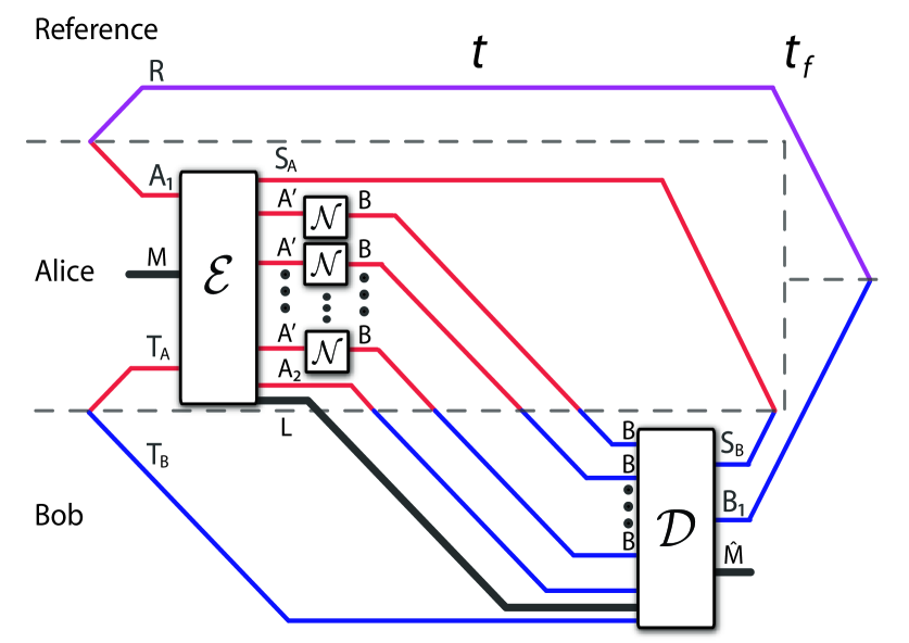
Figure 1: (Color online) The most general protocol for generating classical communication, quantum communication, and entanglement with the help of the same respective resources and many uses of a noisy quantum channel. Alice begins with her classical register $M$, her quantum register $A_{1}$, and her half of the shared entanglement in register $T_{A}$. She encodes according to some CPTP map$\ \mathcal{E}$ that outputs a quantum register $S_{A}$, many registers $A^{\prime n}$, a quantum register $A_{2}$, and a classical register $L$. She inputs $A^{\prime n}$ to many uses of the noisy channel $\mathcal{N}$ and transmits $A_{2}$ over a noiseless quantum channel and $L$ over a noiseless classical channel. Bob receives the channel outputs $B^{n}$, the quantum register $A_{2}$, and the classical register $L$ and performs a decoding $\mathcal{D}$ that recovers the quantum information and classical message. The decoding also generates entanglement with system $S_{A}$. Many protocols are a special case of the above one. For example, the protocol is entanglement-assisted communication of classical and quantum information HW08GFP  if the registers $L$, $S_{A}$, $S_{B}$, and $A_{2}$ are null.

We are interested in the most general protocol that generates classical communication, quantum communication, and entanglement by consuming many uses of a noisy quantum channel $\mathcal{N}^{A^{\prime}\rightarrow B}$ and the same respective resources (see Figure 1). We say that such a protocol is “catalytic” because we are allowing it to consume the same resources that it generates, though we are keeping track of the net rates of consumption or generation.

The protocol begins with Alice possessing two classical registers (each labeled by $M$ and of dimension $2^{n\bar{C}}$), a quantum register $A_{1}$ of dimension $2^{n\bar{Q}}$ entangled with a reference system $R$, and another quantum register $T_{A}$ of dimension $2^{n\tilde{E}}$ that contains her half of the shared entanglement with Bob:

$$\omega^{MMRA_{1}T_{A}T_{B}}\equiv\overline{\Phi}^{MM}\otimes\Phi^{RA_{1}}\otimes\Phi^{T_{A}T_{B}}.$$

She passes one of the classical registers and the registers $A_{1}$ and $T_{A}$ into a CPTP encoding map $\mathcal{E}^{MA_{1}T_{A}\rightarrow A^{\prime n}S_{A}LA_{2}}$ that outputs a quantum register $S_{A}$ of dimension $2^{n\bar{E}}$ and a quantum register $A_{2}$ of dimension $2^{n\tilde{Q}}$, a classical register $L$ of dimension $2^{n\tilde{C}}$, and many quantum systems $A^{\prime n}$ for input to the channel. The register $S_{A}$ is for creating entanglement with Bob. The state after the encoding map $\mathcal{E}$ is as follows:

$$\omega^{MA^{\prime n}S_{A}LA_{2}RT_{B}}\equiv\mathcal{E}^{MA_{1}T_{A}\rightarrow A^{\prime n}S_{A}LA_{2}}(\omega^{MMRA_{1}T_{A}T_{B}}).$$

She sends the systems $A^{\prime n}$ through many uses $\mathcal{N}^{A^{\prime n}\rightarrow B^{n}}$ of the noisy channel $\mathcal{N}^{A^{\prime}\rightarrow B}$, transmits $L$ over a noiseless classical channel, and transmits $A_{2}$ over a noiseless quantum channel, producing the following state:

$$\omega^{MB^{n}S_{A}LA_{2}RT_{B}}\equiv\mathcal{N}^{A^{\prime n}\rightarrow B^{n}}(\omega^{MA^{\prime n}S_{A}LA_{2}RT_{B}}).$$

The above state is a state of the form in (15) with $A\equiv RT_{B}A_{2}S_{A}$ and $X\equiv ML$. Bob then applies a map $\mathcal{D}^{B^{n}A_{2}T_{B}L\rightarrow B_{1}S_{B}\hat{M}}$ that outputs a quantum system $B_{1}$, a quantum system $S_{B}$, and a classical register $\hat{M}$. Let $\omega^{\prime}$ denote the final state. The following condition holds for a good protocol:

$$\left\|\overline{\Phi}^{M\hat{M}}\otimes\Phi^{RB_{1}}\otimes\Phi^{S_{A}S_{B}}-\left(\omega^{\prime}\right)^{MB_{1}S_{B}\hat{M}S_{A}R}\right\|_{1}\leq\epsilon,$$ (4)

implying that Alice and Bob establish maximal classical correlations in $M$ and $\hat{M}$ and maximal entanglement between $S_{A}$ and $S_{B}$. The above condition also implies that the coding scheme preserves the entanglement with the reference system $R$. The net rate triple for the protocol is as follows: $\left(\bar{C}-\tilde{C},\bar{Q}-\tilde{Q},\bar{E}-\tilde{E}\right)$. The protocol generates a resource if its corresponding rate is positive, and it consumes a resource if its corresponding rate is negative. Such a protocol defines an $(n,C,Q,E,\epsilon)$ code with

$$C =\bar{C}-\tilde{C},$$ (5)

$$Q =\bar{Q}-\tilde{Q},$$ (6)

$$E =\bar{E}-\tilde{E}.$$ (7)

Definition 1 (Achievability)

A rate triple $(C,Q,E)$ is achievable if there exists an $(n,C,Q,E,\epsilon)$ code with error (as defined in (4)) smaller than $\epsilon$ for all $\epsilon>0$ and sufficiently large $n$.

Definition 2 (Dynamic Capacity Region)

The dynamic capacity region $\mathcal{C}_{\text{CQE}}\left(\mathcal{N}\right)$ of a noisy quantum channel $\mathcal{N}^{A^{\prime}\rightarrow B}$ is a three-dimensional region in the $(C,Q,E)$ space defined by the closure of the set of all achievable rate triples $(C,Q,E)$.

4 The dynamic capacity theorem

The dynamic capacity theorem gives bounds on the reliable communication rates of a noisy quantum channel when combined with the noiseless resources of classical communication, quantum communication, and shared entanglement HW09T3 . The theorem applies regardless of whether a protocol consumes the noiseless resources or generates them.

Theorem 4.1 (Dynamic Capacity)

The dynamic capacity region $\mathcal{C}_{\text{\emph{CQE}}}(\mathcal{N})$ of a quantum channel $\mathcal{N}$ is equal to the following expression:

$$\mathcal{C}_{\text{\emph{CQE}}}(\mathcal{N})=\overline{\bigcup_{k=1}^{\infty}\frac{1}{k}\mathcal{C}_{\text{\emph{CQE}}}^{(1)}(\mathcal{N}^{\otimes k})},$$ (8)

where the overbar indicates the closure of a set. The “one-shot” region $\mathcal{C}_{\text{\emph{CQE}}}^{(1)}(\mathcal{N})$ is the union of the “one-shot, one-state” regions $\mathcal{C}_{\text{\emph{CQE}},\sigma}^{(1)}(\mathcal{N})$:

$$\mathcal{C}_{\text{\emph{CQE}}}^{(1)}(\mathcal{N})\equiv\bigcup_{\sigma}\mathcal{C}_{\text{\emph{CQE}},\sigma}^{(1)}(\mathcal{N}).$$

The “one-shot, one-state” region $\mathcal{C}_{\text{\emph{CQE}},\sigma}^{(1)}(\mathcal{N})$ is the set of all rates $C$, $Q$, and $E$, such that

$$C+2Q \leq I(AX;B)_{\sigma},$$ (9)

$$Q+E \leq I(A\rangle BX)_{\sigma},$$ (10)

$$C+Q+E \leq I(X;B)_{\sigma}+I(A\rangle BX)_{\sigma}.$$ (11)

The above entropic quantities are with respect to a classical-quantum state $\sigma^{XAB}$ where

$$\sigma^{XAB}\equiv\sum_{x}p(x)\left|x\right\rangle\left\langle x\right|^{X}\otimes\mathcal{N}^{A^{\prime}\rightarrow B}(\phi_{x}^{AA^{\prime}}),$$ (12)

and the states $\phi_{x}^{AA^{\prime}}$ are pure. It is implicit that one should consider states on $A^{\prime k}$ instead of $A^{\prime}$ when taking the regularization in (8).

The above theorem is a “multi-letter” capacity theorem because of the regularization in (8). Though, we show in Sections 8 and 10 that the regularization is not necessary for the Hadamard class of channels or the quantum erasure channels, respectively. We prove the above theorem in two parts:

1. The direct coding theorem below shows that combining the “classically-enhanced father protocol” with teleportation, super-dense coding, and entanglement distribution achieves the above region.

2. The converse theorem demonstrates that any coding scheme cannot do better than the regularization in (8), in the sense that a scheme with vanishing error should have its rates below the above amounts. We prove the converse theorem directly in “one fell swoop,” by employing a catalytic, information-theoretic approach. The converse proof is different from our earlier one HW09T3  because we employ straightforward information-theoretic arguments instead of making contact with prior quantum Shannon theoretic literature.

5 Dynamic achievable rate region

The unit resource achievable region is what Alice and Bob can achieve with the protocols entanglement distribution, teleportation, and super-dense coding HW09T3 . It is the cone of the rate triples corresponding to these protocols:

$$\left\{\alpha\left(0,-1,1\right)+\beta\left(2,-1,-1\right)+\gamma\left(-2,1,-1\right):\alpha,\beta,\gamma\geq 0\right\}.$$

We can also write any rate triple $\left(C,Q,E\right)$ in the unit resource capacity region with a matrix equation:

$$\begin{bmatrix}C\\ Q\\ E\end{bmatrix}=\begin{bmatrix}0&2&-2\\ -1&-1&1\\ 1&-1&-1\end{bmatrix}\begin{bmatrix}\alpha\\ \beta\\ \gamma\end{bmatrix}.$$ (13)

The inverse of the above matrix is as follows:

$$\begin{bmatrix}-\frac{1}{2}&-1&0\\ 0&-\frac{1}{2}&-\frac{1}{2}\\ -\frac{1}{2}&-\frac{1}{2}&-\frac{1}{2}\end{bmatrix},$$

and gives the following set of inequalities for the unit resource achievable region:

$$C+2Q \leq 0,$$

$$Q+E \leq 0,$$

$$C+Q+E \leq 0,$$

by inverting the matrix equation in (13) and applying the constraints $\alpha,\beta,\gamma\geq 0$.

Now, let us include the classically-enhanced father protocol HW08GFP . Ref. HW08GFP proved that we can achieve the following rate triple by channel coding over a noisy quantum channel $\mathcal{N}^{A^{\prime}\rightarrow B}$:

$$\left(I\left(X;B\right)_{\sigma},\frac{1}{2}I\left(A;B|X\right)_{\sigma},-\frac{1}{2}I\left(A;E|X\right)_{\sigma}\right),$$

for any state $\sigma^{XABE}$ of the form:

$$\sigma^{XABE}\equiv\sum_{x}p_{X}\left(x\right)\left|x\right\rangle\left\langle x\right|^{X}\otimes U_{\mathcal{N}}^{A^{\prime}\rightarrow BE}(\phi_{x}^{AA^{\prime}}),$$ (14)

where $U_{\mathcal{N}}^{A^{\prime}\rightarrow BE}$ is an isometric extension of the quantum channel $\mathcal{N}^{A^{\prime}\rightarrow B}$. Specifically, we showed in Ref. HW08GFP  that one can achieve the above rates with vanishing error in the limit of large blocklength. Thus the achievable rate region is the following translation of the unit resource achievable region in (13):

$$\begin{bmatrix}C\\ Q\\ E\end{bmatrix}=\begin{bmatrix}0&2&-2\\ -1&-1&1\\ 1&-1&-1\end{bmatrix}\begin{bmatrix}\alpha\\ \beta\\ \gamma\end{bmatrix}+\begin{bmatrix}I\left(X;B\right)_{\sigma}\\ \frac{1}{2}I\left(A;B|X\right)_{\sigma}\\ -\frac{1}{2}I\left(A;E|X\right)_{\sigma}\end{bmatrix}.$$

We can now determine bounds on an achievable rate region that employs the above coding strategy. We apply the inverse of the matrix in (13) to the LHS and RHS. Then using (2), (3), and the constraints $\alpha,\beta,\gamma\geq 0$, we obtain the inequalities in (9-11), corresponding exactly to the one-shot, one-state region in Theorem 4.1. Taking the union over all possible states $\sigma$ in (14) and taking the regularization gives the full dynamic achievable rate region.

6 Catalytic and information theoretic converse proof

This section begins one of the main contributions of this work. We provide a catalytic, information theoretic converse proof of the dynamic capacity region, showing that (8) gives a multi-letter characterization of it. The catalytic approach means that we are considering the most general protocol that consumes and generates classical communication, quantum communication, and entanglement in addition to the uses of the noisy quantum channel. This approach has the advantage that we can prove the converse theorem in “one fell swoop” rather than considering one octant of the $\left(C,Q,E\right)$ space at a time as we did in Ref. HW09T3 . Additionally, we do not need to make contact with prior work in quantum Shannon theory. We employ the Alicki-Fannes’ inequality, the chain rule for quantum mutual information, elementary properties of quantum entropy, and the quantum data processing inequality to prove the converse.

There are some subtleties in our proof for the converse theorem. We prove that the bounds in (9-11) hold for common randomness generation instead of classical communication because a capacity for generating common randomness can only be better than that for generating classical communication (classical communication can generate common randomness). We also consider a protocol that preserves entanglement with a reference system instead of one that generates quantum communication. Barnum et al. showed that this task is equivalent to the transmission of quantum information BKN98 .

We prove that the converse theorem holds for a state of the following form

$$\sigma^{XAB}\equiv\sum_{x}p(x)\left|x\right\rangle\left\langle x\right|^{X}\otimes\mathcal{N}^{A^{\prime}\rightarrow B}(\rho_{x}^{AA^{\prime}}),$$ (15)

where the states $\rho_{x}^{AA^{\prime}}$ are mixed, rather than proving it for a state of the form in (14). Then we show in Section 6.1 that it is not necessary to consider an ensemble of mixed states—i.e., we can do just as well with an ensemble of pure states, giving the statement of Theorem 4.1.

We begin by proving the first bound in (9). All system labels are as given in Section 3, and we consider the most general protocol as outlined in that section. Consider the following chain of inequalities:

$$n\left(\bar{C}+2\bar{Q}\right) =I(M;\hat{M})_{\overline{\Phi}}+I\left(R;B_{1}\right)_{\Phi}$$

$$\leq I(M;\hat{M})_{\omega^{\prime}}+I\left(R;B_{1}\right)_{\omega^{\prime}}+n\delta^{\prime}$$

$$\leq I\left(M;B^{n}A_{2}LT_{B}\right)_{\omega}+I\left(R;B^{n}A_{2}LT_{B}\right)_{\omega}$$

$$\leq I\left(M;B^{n}A_{2}LT_{B}\right)_{\omega}+I\left(R;B^{n}A_{2}LT_{B}M\right)_{\omega}$$

$$=I\left(M;B^{n}A_{2}LT_{B}\right)_{\omega}+I\left(R;B^{n}A_{2}LT_{B}|M\right)_{\omega}+I\left(R;M\right)_{\omega}.$$

The first equality holds by evaluating the quantum mutual informations on the respective states $\overline{\Phi}^{M\hat{M}}$ and $\Phi^{RB_{1}}$. The first inequality follows from the condition in (4) and an application of the Alicki-Fannes’ inequality where $\delta^{\prime}$ vanishes as $\epsilon\rightarrow 0$. We suppress this term in the rest of the inequalities for convenience. The second inequality follows from quantum data processing, and the third follows from another application of quantum data processing. The second equality follows by applying the mutual information chain rule in (1). We continue below:

$$=I\left(M;B^{n}A_{2}LT_{B}\right)_{\omega}+I\left(R;B^{n}A_{2}LT_{B}|M\right)_{\omega}$$

$$=I\left(M;B^{n}A_{2}LT_{B}\right)_{\omega}+I\left(RA_{2}LT_{B};B^{n}|M\right)_{\omega}+I\left(R;A_{2}LT_{B}|M\right)_{\omega}-I\left(B^{n};A_{2}LT_{B}|M\right)_{\omega}$$

$$=I\left(M;B^{n}\right)_{\omega}+I\left(M;A_{2}LT_{B}|B^{n}\right)_{\omega}+I\left(RA_{2}LT_{B};B^{n}|M\right)_{\omega}+I\left(R;A_{2}LT_{B}|M\right)_{\omega}-I\left(B^{n};A_{2}LT_{B}|M\right)_{\omega}$$

$$=I\left(RA_{2}LMT_{B};B^{n}\right)_{\omega}+I\left(M;A_{2}LT_{B}|B^{n}\right)_{\omega}+I\left(R;A_{2}LT_{B}|M\right)_{\omega}-I\left(B^{n};A_{2}LT_{B}|M\right)_{\omega}$$

$$\leq I\left(RA_{2}T_{B}S_{A}LM;B^{n}\right)_{\omega}+I\left(M;A_{2}LT_{B}|B^{n}\right)_{\omega}+I\left(R;A_{2}LT_{B}|M\right)_{\omega}-I\left(B^{n};A_{2}LT_{B}|M\right)_{\omega}$$

$$=I\left(AX;B^{n}\right)_{\omega}+I\left(M;A_{2}LT_{B}|B^{n}\right)_{\omega}+I\left(R;A_{2}LT_{B}|M\right)_{\omega}-I\left(B^{n};A_{2}LT_{B}|M\right)_{\omega}.$$

The first equality follows because $I\left(R;M\right)_{\omega}=0$ for this protocol. The second equality follows from applying the chain rule for quantum mutual information to the term $I\left(R;B^{n}A_{2}LT_{B}|M\right)_{\omega}$, and the third is another application of the chain rule to the term $I\left(M;B^{n}A_{2}LT_{B}\right)_{\omega}$. The fourth equality follows by combining $I\left(M;B^{n}\right)_{\omega}$ and $I\left(RA_{2}LT_{B};B^{n}|M\right)_{\omega}$ with the chain rule. The inequality follows from an application of quantum data processing. The final equality follows from the definitions $A\equiv RT_{B}A_{2}S_{A}$ and $X\equiv ML$. We now focus on the term $I\left(M;A_{2}LT_{B}|B^{n}\right)_{\omega}+I\left(R;A_{2}LT_{B}|M\right)_{\omega}-I\left(B^{n};A_{2}LT_{B}|M\right)_{\omega}$ and show that it is less than $n\left(\tilde{C}+2\tilde{Q}\right)$:

$$I\left(M;A_{2}LT_{B}|B^{n}\right)_{\omega}+I\left(R;A_{2}LT_{B}|M\right)_{\omega}-I\left(B^{n};A_{2}LT_{B}|M\right)_{\omega}$$

$$=I\left(M;A_{2}LT_{B}B^{n}\right)_{\omega}+I\left(R;A_{2}LT_{B}M\right)_{\omega}-I\left(B^{n};A_{2}LT_{B}M\right)_{\omega}-I\left(R;M\right)_{\omega}$$

$$=I\left(M;A_{2}LT_{B}B^{n}\right)_{\omega}+I\left(R;A_{2}LT_{B}M\right)_{\omega}-I\left(B^{n};A_{2}LT_{B}M\right)_{\omega}$$

$$=H\left(A_{2}LT_{B}B^{n}\right)_{\omega}+H\left(R\right)_{\omega}-H\left(RA_{2}LT_{B}|M\right)_{\omega}-H\left(B^{n}\right)_{\omega}$$

$$=H\left(A_{2}LT_{B}B^{n}\right)_{\omega}-H\left(A_{2}LT_{B}|MR\right)_{\omega}-H\left(B^{n}\right)_{\omega}$$

$$=H\left(A_{2}LT_{B}|B^{n}\right)_{\omega}-H\left(A_{2}LT_{B}|MR\right)_{\omega}.$$

The first equality follows by applying the chain rule for quantum mutual information. The second equality follows because $I\left(R;M\right)_{\omega}=0$ for this protocol. The third equality follows by expanding the quantum mutual informations. The next two inequalities follow from straightforward entropic manipulations and that $H\left(R\right)_{\omega}=H\left(R|M\right)_{\omega}$ for this protocol. We continue below:

$$=H\left(A_{2}L|B^{n}\right)_{\omega}+H\left(T_{B}|B^{n}A_{2}L\right)_{\omega}-H\left(T_{B}|MR\right)_{\omega}-H\left(A_{2}L|T_{B}MR\right)_{\omega}$$

$$=H\left(A_{2}L|B^{n}\right)_{\omega}+H\left(T_{B}|B^{n}A_{2}L\right)_{\omega}-H\left(T_{B}\right)_{\omega}-H\left(A_{2}L|T_{B}MR\right)_{\omega}$$

$$=H\left(A_{2}L|B^{n}\right)_{\omega}-I\left(T_{B};B^{n}A_{2}L\right)_{\omega}-H\left(A_{2}L|T_{B}MR\right)$$

$$\leq H\left(A_{2}L\right)_{\omega}-H\left(A_{2}L|T_{B}MR\right)_{\omega}$$

$$=I\left(A_{2}L;T_{B}MR\right)_{\omega}$$

$$=I\left(L;T_{B}MR\right)_{\omega}+I\left(A_{2};T_{B}MR|L\right)_{\omega}$$

$$\leq n\left(\tilde{C}+2\tilde{Q}\right).$$

The first two equalities follow from the chain rule for entropy and the second exploits that $H\left(T_{B}|MR\right)=H\left(T_{B}\right)$ for this protocol. The third equality follows from the definition of quantum mutual information. The inequality follows from subadditivity of entropy and that $I\left(T_{B};B^{n}A_{2}L\right)_{\omega}\geq 0$. The fourth equality follows from the definition of quantum mutual information and the next equality follows from the chain rule. The final inequality follows because the quantum mutual information $I\left(L;T_{B}MR\right)_{\omega}$ can never be larger than the logarithm of the dimension of the classical register $L$ and because the quantum mutual information $I\left(A_{2};T_{B}MR|L\right)_{\omega}$ can never be larger than twice the logarithm of the dimension of the quantum register $A_{2}$. Thus the following inequality applies

$$n\left(\bar{C}+2\bar{Q}\right)\leq I\left(AX;B^{n}\right)_{\omega}+n\left(\tilde{C}+2\tilde{Q}\right)+n\delta^{\prime},$$

demonstrating that (9) holds for the net rates.

We now prove the second bound in (10). Consider the following chain of inequalities:

$$n\left(\bar{Q}+\bar{E}\right) =I\left(R\rangle B_{1}\right)_{\Phi}+I\left(S_{A}\rangle S_{B}\right)_{\Phi}$$

$$=I\left(RS_{A}\rangle B_{1}S_{B}\right)_{\Phi\otimes\Phi}$$

$$\leq I\left(RS_{A}\rangle B_{1}S_{B}\right)_{\omega^{\prime}}+n\delta^{\prime}$$

$$\leq I\left(RS_{A}\rangle B_{1}S_{B}M\right)_{\omega^{\prime}}$$

$$\leq I\left(RS_{A}\rangle B^{n}A_{2}T_{B}LM\right)_{\omega}$$

$$=H\left(B^{n}A_{2}T_{B}|LM\right)_{\omega}-H\left(RS_{A}B^{n}A_{2}T_{B}|LM\right)_{\omega}$$

$$\leq H\left(B^{n}|LM\right)_{\omega}+H\left(A_{2}|LM\right)_{\omega}+H\left(T_{B}|LM\right)_{\omega}-H\left(RS_{A}B^{n}A_{2}T_{B}|LM\right)_{\omega}$$

$$\leq I\left(RS_{A}A_{2}T_{B}\rangle B^{n}LM\right)_{\omega}+n\left(\tilde{Q}+\tilde{E}\right)$$

$$=I\left(A\rangle B^{n}X\right)_{\omega}+n\left(\tilde{Q}+\tilde{E}\right).$$

The first equality follows by evaluating the coherent informations of the respective states $\Phi^{RB_{1}}$ and $\Phi^{S_{A}S_{B}}$. The second equality follows because $\Phi^{RB_{1}}\otimes\Phi^{T_{A}T_{B}}$ is a product state. The first inequality follows from the condition in (4) and an application of the Alicki-Fannes’ inequality with $\delta^{\prime}$ vanishing when $\epsilon\rightarrow 0$. We suppress the term $n\delta^{\prime}$ in the following lines. The next two inequalities follow from quantum data processing. The third equality follows from the definition of coherent information. The fourth inequality follows from subadditivity of entropy. The fifth inequality follows from the definition of coherent information and the fact that the entropy can never be larger than the logarithm of the dimension of the corresponding system. The final equality follows from the definitions $A\equiv RT_{B}A_{2}S_{A}$ and $X\equiv ML$. Thus the following inequality applies

$$n\left(\bar{Q}+\bar{E}\right)\leq I\left(A\rangle B^{n}X\right)+n\left(\tilde{Q}+\tilde{E}\right),$$

demonstrating that (10) holds for the net rates.

We prove the last bound in (11). Consider the following chain of inequalities:

$$n\left(\bar{C}+\bar{Q}+\bar{E}\right) =I(M;\hat{M})_{\overline{\Phi}}+I\left(RS_{A}\rangle B_{1}S_{B}\right)_{\Phi\otimes\Phi}$$

$$\leq I(M;\hat{M})_{\omega^{\prime}}+I\left(RS_{A}\rangle B_{1}S_{B}\right)_{\omega^{\prime}}+n\delta^{\prime}$$

$$\leq I(M;B^{n}A_{2}T_{B}L)_{\omega}+I\left(RS_{A}\rangle B^{n}A_{2}T_{B}LM\right)_{\omega}$$

$$=I\left(ML;B^{n}A_{2}T_{B}\right)_{\omega}+I\left(M;L\right)_{\omega}-I\left(A_{2}B^{n}T_{B};L\right)_{\omega}$$

$$\ \ \ \ \ \ +H\left(B^{n}|LM\right)+H\left(A_{2}T_{B}|B^{n}LM\right)_{\omega}-H\left(RS_{A}A_{2}T_{B}B^{n}|LM\right)_{\omega}$$

$$=I\left(ML;B^{n}\right)_{\omega}+I\left(ML;A_{2}T_{B}|B^{n}\right)_{\omega}+I\left(M;L\right)_{\omega}-I\left(A_{2}B^{n}T_{B};L\right)_{\omega}$$

$$\ \ \ \ \ \ +H\left(A_{2}T_{B}|B^{n}LM\right)_{\omega}+I\left(RS_{A}A_{2}T_{B}\rangle B^{n}LM\right)_{\omega}.$$

The first equality follows from evaluating the mutual information of the state $\overline{\Phi}^{M\hat{M}}$ and the coherent information of the product state $\Phi^{RB_{1}}\otimes\Phi^{S_{A}S_{B}}$. The first inequality follows from the condition in (4) and an application of the Alicki-Fannes’ inequality with $\delta^{\prime}$ vanishing when $\epsilon\rightarrow 0$. We suppress the term $n\delta^{\prime}$ in the following lines. The second inequality follows from quantum data processing. The second equality follows from applying the chain rule for quantum mutual information to $I(M;B^{n}A_{2}T_{B}L)_{\omega}$ and by expanding the coherent information $I\left(RS_{A}\rangle B^{n}A_{2}T_{B}LM\right)_{\omega}$. The third equality follows from applying the chain rule for quantum mutual information to $I\left(ML;B^{n}A_{2}T_{B}\right)_{\omega}$ and from the definition of coherent information. We continue below:

$$=I\left(ML;B^{n}\right)_{\omega}+I\left(RS_{A}A_{2}T_{B}\rangle B^{n}LM\right)_{\omega}$$

$$\ \ \ \ \ \ +I\left(ML;A_{2}T_{B}|B^{n}\right)_{\omega}+I\left(M;L\right)_{\omega}-I\left(A_{2}B^{n}T_{B};L\right)_{\omega}+H\left(A_{2}T_{B}|B^{n}LM\right)_{\omega}$$

$$=I\left(ML;B^{n}\right)_{\omega}+I\left(RS_{A}A_{2}T_{B}\rangle B^{n}LM\right)_{\omega}$$

$$\ \ \ \ \ \ +H\left(A_{2}T_{B}|B^{n}\right)_{\omega}+I\left(M;L\right)_{\omega}-I\left(A_{2}B^{n}T_{B};L\right)_{\omega}$$

$$\leq I\left(ML;B^{n}\right)_{\omega}+I\left(RS_{A}A_{2}T_{B}\rangle B^{n}LM\right)_{\omega}+n\left(\tilde{C}+\tilde{Q}+\tilde{E}\right)$$

$$=I\left(X;B^{n}\right)_{\omega}+I\left(A\rangle B^{n}X\right)_{\omega}+n\left(\tilde{C}+\tilde{Q}+\tilde{E}\right).$$

The first equality follows by rearranging terms. The second equality follows by canceling terms. The inequality follows from subadditivity of the entropy $H\left(A_{2}T_{B}|B^{n}\right)_{\omega}$, the fact that the entropy $H\left(A_{2}T_{B}|B^{n}\right)_{\omega}$ can never be larger than the logarithm of the dimension of the systems $A_{2}T_{B}$, that the mutual information $I\left(M;L\right)_{\omega}$ can never be larger than the logarithm of the dimension of the classical register $L$, and because $I\left(A_{2}B^{n}T_{B};L\right)_{\omega}\geq 0$. The last equality follows from the definitions $A\equiv RT_{B}A_{2}S_{A}$ and $X\equiv ML$. Thus the following inequality holds

$$n\left(\bar{C}+\bar{Q}+\bar{E}\right)\leq I\left(X;B^{n}\right)_{\omega}+I\left(A\rangle B^{n}X\right)_{\omega}+n\left(\tilde{C}+\tilde{Q}+\tilde{E}\right)+n\delta^{\prime},$$

demonstrating that the inequality in (11) applies to the net rates. This concludes the catalytic proof of the converse theorem.

6.1 Pure state ensembles are sufficient

We prove that it is sufficient to consider an ensemble of pure states as in the statement of Theorem 4.1 rather than an ensemble of mixed states as in (15) in the proof of our converse theorem. Our argument relies on a classic trick exploited in quantum Shannon theory DHW05RI . We first determine a spectral decomposition of the mixed state ensemble, model the index of the pure states in the decomposition as a classical variable $Y$, and then place this classical variable $Y$ in a classical register. It follows that the communication rates can only improve, and it is sufficient to consider an ensemble of pure states.

Consider that each mixed state in the ensemble in (15) admits a spectral decomposition of the following form:

$$\rho_{x}^{AA^{\prime}}=\sum_{y}p\left(y|x\right)\psi_{x,y}^{AA^{\prime}}.$$

We can thus represent the ensemble as follows:

$$\rho^{XAB}\equiv\sum_{x,y}p(x)p\left(y|x\right)\left|x\right\rangle\left\langle x\right|^{X}\otimes\mathcal{N}^{A^{\prime}\rightarrow B}(\psi_{x,y}^{AA^{\prime}}).$$ (16)

The inequalities in (9-11) for the dynamic capacity region involve the mutual information $I(AX;B)_{\rho}$, the Holevo information $I(X;B)_{\rho}$, and the coherent information $I(A\rangle BX)_{\rho}$. As we show below, each of these entropic quantities can only improve in each case if make the variable $y$ be part of the classical variable. This improvement then implies that it is only necessary to consider pure states in the dynamic capacity theorem.

Let $\theta^{XYAB}$ denote an augmented state of the following form:

$$\theta^{XYAB}\equiv\sum_{x}p(x)p\left(y|x\right)\left|x\right\rangle\left\langle x\right|^{X}\otimes\left|y\right\rangle\left\langle y\right|^{Y}\otimes\mathcal{N}^{A^{\prime}\rightarrow B}(\psi_{x,y}^{AA^{\prime}}).$$ (17)

This state is actually a state of the form in (12) if we subsume the classical variables $X$ and $Y$ into one classical variable. The following three inequalities each follow from an application of the quantum data processing inequality:

$$I(X;B)_{\rho} =I(X;B)_{\theta}\leq I(XY;B)_{\theta},$$ (18)

$$I(AX;B)_{\rho} =I(AX;B)_{\theta}\leq I(AXY;B)_{\theta}$$ (19)

$$I(A\rangle BX)_{\rho} =I(A\rangle BX)_{\theta}\leq I(A\rangle BXY)_{\theta}.$$ (20)

Each of these inequalities proves the desired result for the respective Holevo information, mutual information, and coherent information, and it suffices to consider an ensemble of pure states in Theorem 4.1.

7 The quantum dynamic capacity formula

We introduce the quantum dynamic capacity formula and show how additivity of it implies that the computation of the Pareto optimal trade-off surface of the capacity region requires just a single channel use, rather than an infinite number of them (as in regularized formulas). The Pareto optimal trade-off surface consists of all points in the capacity region that are Pareto optimal, in the sense that it is not possible to make improvements in one resource without offsetting another resource (these are essentially the boundary points of the region in our case). We then show how several important capacity formulas in the quantum Shannon theory literature are special cases of the quantum dynamic capacity formula.

Definition 3 (Quantum Dynamic Capacity Formula)

The quantum dynamic capacity formula of a quantum channel $\mathcal{N}$ is as follows:

$$D_{\lambda,\mu}\left(\mathcal{N}\right)\equiv\max_{\sigma}I\left(AX;B\right)_{\sigma}+\lambda I\left(A\rangle BX\right)_{\sigma}+\mu\left(I\left(X;B\right)_{\sigma}+I\left(A\rangle BX\right)_{\sigma}\right),$$ (21)

where $\lambda,\mu\geq 0$.

Definition 4

The regularized quantum dynamic capacity formula is as follows:

$$D_{\lambda,\mu}^{\text{reg}}\left(\mathcal{N}\right)\equiv\lim_{n\rightarrow\infty}\frac{1}{n}D_{\lambda,\mu}\left(\mathcal{N}^{\otimes n}\right).$$

Lemma 1

Suppose the quantum dynamic capacity formula is additive for any two channels $\mathcal{N}$ and $\mathcal{M}$:

$$D_{\lambda,\mu}\left(\mathcal{N\otimes M}\right)=D_{\lambda,\mu}\left(\mathcal{N}\right)+D_{\lambda,\mu}\left(\mathcal{M}\right).$$

Then the regularized quantum dynamic capacity formula for $\mathcal{N}$ is equal to the quantum dynamic capacity formula for $\mathcal{N}$:

$$D_{\lambda,\mu}^{\text{reg}}\left(\mathcal{N}\right)=D_{\lambda,\mu}\left(\mathcal{N}\right).$$

In this sense, the regularized formula “single-letterizes” and it is not necessary to take the limit.

Proof

We prove the result using induction on $n$. The base case for $n=1$ is trivial. Suppose the result holds for $n$: $D_{\lambda,\mu}(\mathcal{N}^{\otimes n})=nD_{\lambda,\mu}(\mathcal{N})$. Then the following chain of equalities proves the inductive step:

$$D_{\lambda,\mu}(\mathcal{N}^{\otimes n+1}) =D_{\lambda,\mu}(\mathcal{N}\otimes\mathcal{N}^{\otimes n})$$

$$=D_{\lambda,\mu}(\mathcal{N})+D_{\lambda,\mu}(\mathcal{N}^{\otimes n})$$

$$=D_{\lambda,\mu}(\mathcal{N})+nD_{\lambda,\mu}(\mathcal{N}).$$

The first equality follows by expanding the tensor product. The second critical equality follows from the assumption that the formula is additive. The final equality follows from the induction hypothesis.

Theorem 7.1

Single-letterization of the quantum dynamic capacity formula implies that the computation of the Pareto optimal trade-off surface of the quantum dynamic capacity region requires an optimization over a single channel use.

Proof

We employ ideas from Ref. BV04 for the proof. We would like to characterize all the points in the capacity region that are Pareto optimal. Such a task is standard vector optimization in the theory of Pareto trade-off analysis (see Section 4.7 of Ref. BV04 ). We can phrase the optimization task as the following scalarization of the vector optimization task:

$$\max_{C,Q,E,p\left(x\right),\phi_{x}}w_{C}C+w_{Q}Q+w_{E}E$$ (22)

subject to

$$C+2Q \leq I(AX;B^{n})_{\sigma},$$ (23)

$$Q+E \leq I(A\rangle B^{n}X)_{\sigma},$$ (24)

$$C+Q+E \leq I(X;B^{n})_{\sigma}+I(A\rangle B^{n}X)_{\sigma},$$ (25)

where the maximization is over all $C$, $Q$, and $E$ and over probability distributions $p_{X}\left(x\right)$ and bipartite states $\phi_{x}^{AA^{\prime n}}$. The geometric interpretation of the scalarization task is that we are trying to find a supporting plane of the dynamic capacity region where the weight vector $\left(w_{C},w_{Q},w_{E}\right)$ is the normal vector of the plane and the value of its inner product with $\left(C,Q,E\right)$ characterizes the offset of the plane.

The Lagrangian of the above optimization problem is

$$\mathcal{L}\left(C,Q,E,p_{X}\left(x\right),\phi_{x}^{AA^{\prime n}},\lambda_{1},\lambda_{2},\lambda_{3}\right) \equiv w_{C}C+w_{Q}Q+w_{E}E+\lambda_{1}\left(I\left(AX;B^{n}\right)_{\sigma}-\left(C+2Q\right)\right)$$

$$\ \ \ \ \ \ +\lambda_{2}\left(I\left(A\rangle B^{n}X\right)_{\sigma}-\left(Q+E\right)\right)$$

$$\ \ \ \ \ \ \ +\lambda_{3}\left(I\left(X;B^{n}\right)_{\sigma}+I\left(A\rangle B^{n}X\right)_{\sigma}-\left(C+Q+E\right)\right),$$

and the Lagrange dual function $g$ BV04 is

$$g\left(\lambda_{1},\lambda_{2},\lambda_{3}\right)\equiv\sup_{C,Q,E,p\left(x\right),\phi_{x}^{AA^{\prime n}}}\mathcal{L}\left(C,Q,E,p_{X}\left(x\right),\phi_{x}^{AA^{\prime n}},\lambda_{1},\lambda_{2},\lambda_{3}\right),$$

where $\lambda_{1},\lambda_{2},\lambda_{3}\geq 0$. The optimization task simplifies if the Lagrange dual function does. Thus, we rewrite the Lagrange dual function as follows:

$$g\left(\lambda_{1},\lambda_{2},\lambda_{3}\right) =\sup_{C,Q,E,p\left(x\right),\phi_{x}^{AA^{\prime n}}}w_{C}C+w_{Q}Q+w_{E}E+\lambda_{1}\left(I\left(AX;B^{n}\right)_{\sigma}-\left(C+2Q\right)\right)$$

$$\ \ \ \ \ \ \ +\lambda_{2}\left(I\left(A\rangle B^{n}X\right)_{\sigma}-\left(Q+E\right)\right)$$

$$\ \ \ \ \ \ \ +\lambda_{3}\left(I\left(X;B^{n}\right)_{\sigma}+I\left(A\rangle B^{n}X\right)_{\sigma}-\left(C+Q+E\right)\right)$$

$$=\sup_{C,Q,E,p\left(x\right),\phi_{x}^{AA^{\prime n}}}\left(w_{C}-\lambda_{1}-\lambda_{3}\right)C+\left(w_{Q}-2\lambda_{1}-\lambda_{2}-\lambda_{3}\right)Q+\left(w_{E}-\lambda_{2}-\lambda_{3}\right)E$$

$$\ \ \ \ \ \ \ +\lambda_{1}\left(I\left(AX;B^{n}\right)_{\sigma}+\frac{\lambda_{2}}{\lambda_{1}}I\left(A\rangle B^{n}X\right)_{\sigma}+\frac{\lambda_{3}}{\lambda_{1}}\left(I\left(X;B^{n}\right)_{\sigma}+I\left(A\rangle B^{n}X\right)_{\sigma}\right)\right)$$

$$=\sup_{C,Q,E}\left(w_{C}-\lambda_{1}-\lambda_{3}\right)C+\left(w_{Q}-2\lambda_{1}-\lambda_{2}-\lambda_{3}\right)Q+\left(w_{E}-\lambda_{2}-\lambda_{3}\right)E$$

$$\ \ \ \ \ \ \ +\lambda_{1}\left(\max_{p\left(x\right),\phi_{x}^{AA^{\prime n}}}I\left(AX;B^{n}\right)_{\sigma}+\frac{\lambda_{2}}{\lambda_{1}}I\left(A\rangle B^{n}X\right)_{\sigma}+\frac{\lambda_{3}}{\lambda_{1}}\left(I\left(X;B^{n}\right)_{\sigma}+I\left(A\rangle B^{n}X\right)_{\sigma}\right)\right).$$

The first equality follows by definition. The second equality follows from some algebra, and the last follows because the Lagrange dual function factors into two separate optimization tasks: one over $C$, $Q$, and $E$ and another that is equivalent to the quantum dynamic capacity formula with $\lambda=\lambda_{2}/\lambda_{1}$ and $\mu=\lambda_{3}/\lambda_{1}$. Thus, the computation of the Pareto optimal trade-off surface requires just a single use of the channel if the quantum dynamic capacity formula in (21) single-letterizes.

7.1 Special cases of the quantum dynamic capacity formula

We now show how several capacity formulas of a quantum channel, including the entanglement-assisted classical capacity BSST01 , the Lloyd-Shor-Devetak (LSD) formula for the quantum capacity Lloyd96 ; Shor02 ; Devetak03 , and the Holevo-Schumacher-Westmoreland (HSW) formula for the classical capacity Hol98 ; SW97 are special cases of the quantum dynamic capacity formula.

We first give a geometric interpretation of these special cases before proceeding to the proofs. Recall that the dynamic capacity region has the simple interpretation as a translation of the three-faced unit resource capacity region along the classically-enhanced father trade-off curve (see Figure 2 for the example of the region of the dephasing channel). Any particular weight vector $\left(w_{C},w_{Q},w_{E}\right)$ in (22) gives a set of parallel planes that slice through the $\left(C,Q,E\right)$ space, and the goal of the scalar optimization task is to find one of these planes that is a supporting plane, intersecting a point (or a set of points) on the trade-off surface of the dynamic capacity region. We consider three special planes:

1. The first corresponds to the plane containing the vectors of super-dense coding and teleportation. The normal vector of this plane is $(1,2,0)$, and suppose that we set the weight vector in (22) to be this vector. Then the optimization program finds the set of points on the trade-off surface such that a plane with this normal vector is a supporting plane for the region. The optimization program singles out (23), and we can think of this as being equivalent to setting $\lambda_{2},\lambda_{3}=0$ in the Lagrange dual function. We show below that the optimization program becomes equivalent to finding the entanglement-assisted capacity BSST01 , in the sense that the quantum dynamic capacity formula becomes the entanglement-assisted capacity formula.

2. The next plane contains the vectors of teleportation and entanglement distribution. The normal vector of this plane is $\left(0,1,1\right)$. Setting the weight vector in (22) to be this vector makes the optimization program single out (24), and we can think of this as being equivalent to setting $\lambda_{1},\lambda_{3}=0$ in the Lagrange dual function. We show below that the optimization program becomes equivalent to finding the quantum capacity Lloyd96 ; Shor02 ; Devetak03 , in the sense that the quantum dynamic capacity formula becomes the LSD formula for the quantum capacity.

3. A third plane contains the vectors of super-dense coding and entanglement distribution. The normal vector of this plane is $\left(1,1,1\right)$. Setting the weight vector in (22) to be this vector makes the optimization program single out (25), and we can think of this as being equivalent to setting $\lambda_{1},\lambda_{2}=0$ in the Lagrange dual function. We show below that the optimization becomes equivalent to finding the classical capacity Lloyd96 ; Shor02 ; Devetak03 , in the sense that the quantum dynamic capacity formula becomes the HSW formula for the classical capacity.

Corollary 1

The quantum dynamic capacity formula is equivalent to the entanglement-assisted classical capacity formula when $\lambda,\mu=0$, in the sense that

$$\max_{\sigma}I\left(AX;B\right)=\max_{\phi^{AA^{\prime}}}I\left(A;B\right).$$

Proof

The inequality $\max_{\sigma}I\left(AX;B\right)\geq\max_{\phi^{AA^{\prime}}}I\left(A;B\right)$ follows because the state $\sigma$ is of the form in (14) and we can always choose $p_{X}\left(x\right)=\delta_{x,x_{0}}$ and $\phi_{x_{0}}^{AA^{\prime}}$ to be the state that maximizes $I\left(A;B\right)$.

We now show the other inequality $\max_{\sigma}I\left(AX;B\right)\leq\max_{\phi^{AA^{\prime}}}I\left(A;B\right)$. First, consider that the following chain of equalities holds for any state $\phi^{ABE}$ resulting from the isometric extension of the channel:

$$I\left(A;B\right) =H\left(B\right)+H\left(A\right)-H\left(AB\right)$$

$$=H\left(B\right)+H\left(BE\right)-H\left(E\right)$$

$$=H\left(B\right)+H\left(B|E\right).$$

In this way, we see that the mutual information is purely a function of the channel input density operator Tr${}_{A}\left\{\phi^{AA^{\prime}}\right\}$. Then consider any state $\sigma$ of the form in (14). The following chain of inequalities holds

$$I\left(AX;B\right)_{\sigma} =H\left(A|X\right)_{\sigma}+H\left(B\right)_{\sigma}-H\left(E|X\right)_{\sigma}$$

$$=H\left(BE|X\right)_{\sigma}+H\left(B\right)_{\sigma}-H\left(E|X\right)_{\sigma}$$

$$=H\left(B|EX\right)_{\sigma}+H\left(B\right)_{\sigma}$$

$$\leq H\left(B|E\right)_{\sigma}+H\left(B\right)_{\sigma}$$

$$\leq\max_{\phi^{AA^{\prime}}}I\left(A;B\right).$$

The first equality follows by expanding the mutual information. The second equality follows because the state on $ABE$ is pure when conditioned on $X$. The third equality follows from the entropy chain rule. The first inequality follows from strong subadditivity, and the last follows because the state after tracing out systems $X$ and $A$ is a particular state that arises from the channel and cannot be larger than the maximum.

Corollary 2

The quantum dynamic capacity formula is equivalent to the LSD quantum capacity formula in the limit where $\lambda\rightarrow\infty$ and $\mu$ is fixed, in the sense that

$$\max_{\sigma}I\left(A\rangle BX\right)=\max_{\phi^{AA^{\prime}}}I\left(A\rangle B\right).$$

Proof

The inequality $\max_{\sigma}I\left(A\rangle BX\right)\geq\max_{\phi^{AA^{\prime}}}I\left(A\rangle B\right)$ follows because the state $\sigma$ is of the form in (14) and we can always choose $p_{X}\left(x\right)=\delta_{x,x_{0}}$ and $\phi_{x_{0}}^{AA^{\prime}}$ to be the state that maximizes $I\left(A\rangle B\right)$.

The inequality $\max_{\sigma}I\left(A\rangle BX\right)\leq\max_{\phi^{AA^{\prime}}}I\left(A\rangle B\right)$ follows because $I\left(A\rangle BX\right)=\sum_{x}p_{X}\left(x\right)I\left(A\rangle B\right)_{\phi_{x}}$ and the maximum is always greater than the average.

Corollary 3

The quantum dynamic capacity formula is equivalent to the HSW classical capacity formula in the limit where $\mu\rightarrow\infty$ and $\lambda$ is fixed, in the sense that

$$\max_{\sigma}I\left(A\rangle BX\right)_{\sigma}+I\left(X;B\right)_{\sigma}=\max_{\left\{p_{X}\left(x\right),\psi_{x}\right\}}I\left(X;B\right).$$

The inequality $\max_{\sigma}I\left(A\rangle BX\right)_{\sigma}+I\left(X;B\right)_{\sigma}\geq\max_{\left\{p_{X}\left(x\right),\psi_{x}\right\}}I\left(X;B\right)$ follows by choosing $\sigma$ to be the pure ensemble that maximizes $I\left(X;B\right)$ and noting that $I\left(A\rangle BX\right)_{\sigma}$ vanishes for a pure ensemble.

We now prove the inequality $\max_{\sigma}I\left(A\rangle BX\right)_{\sigma}+I\left(X;B\right)_{\sigma}\leq\max_{\left\{p_{X}\left(x\right),\psi_{x}\right\}}I\left(X;B\right)$. Consider a state $\omega^{XYBE}$ obtained by performing a von Neumann measurement on the $A$ system of the state $\sigma^{XABE}$. Then

$$I\left(A\rangle BX\right)_{\sigma}+I\left(X;B\right)_{\sigma} =H\left(B\right)_{\sigma}-H\left(E|X\right)_{\sigma}$$

$$=H\left(B\right)_{\omega}-H\left(E|X\right)_{\omega}$$

$$\leq H\left(B\right)_{\omega}-H\left(E|XY\right)_{\omega}$$

$$=H\left(B\right)_{\omega}-H\left(B|XY\right)_{\omega}$$

$$=I\left(XY;B\right)_{\omega}$$

$$\leq\max_{\left\{p_{X}\left(x\right),\psi_{x}\right\}}I\left(X;B\right).$$

The first equality follows by expanding the conditional coherent information and the Holevo information. The second equality follows because the measured $A$ system is not involved in the entropies. The first inequality follows because conditioning does not increase entropy. The third equality follows because the state $\omega$ is pure when conditioned on $X$ and $Y$. The fourth equality follows by definition, and the last inequality follows for clear reasons.

8 Single-letter dynamic capacity region for the quantum Hadamard channels

Below we show that the regularization in (8) is not necessary if the quantum channel is a Hadamard channel. This result holds because a Hadamard channel has a special structure. The development of the proof is similar to that in Ref. BHTW10 , but simplified because we obtain the single-letter result more directly.

Theorem 8.1

The dynamic capacity region $\mathcal{C}_{\mathrm{{CQE}}}(\mathcal{N}_{\text{H}})$ of a quantum Hadamard channel $\mathcal{N}_{\text{H}}$ is equal to its one-shot region $\mathcal{C}_{\mathrm{{CQE}}}^{(1)}(\mathcal{N}_{\text{H}})$.

The proof of the above theorem follows in two parts: 1) the below lemma shows the quantum dynamic capacity formula is additive when one of the channels is Hadamard and 2) the induction argument in Lemma 1 that proves single-letterization.

Lemma 2

The following additivity relation holds for a Hadamard channel $\mathcal{N}_{H}$ and any other channel $\mathcal{N}$:

$$D_{\lambda,\mu}(\mathcal{N}_{H}\otimes\mathcal{N})=D_{\lambda,\mu}(\mathcal{N}_{H})+D_{\lambda,\mu}(\mathcal{N}).$$

Proof

We first note that the inequality $D_{\lambda,\mu}(\mathcal{N}_{H}\otimes\mathcal{N})\geq D_{\lambda,\mu}(\mathcal{N}_{H})+D_{\lambda,\mu}(\mathcal{N})$ holds for any two channels simply by selecting the state $\sigma$ in the maximization to be a tensor product of the ones that individually maximize $D_{\lambda,\mu}(\mathcal{N}_{H})$ and $D_{\lambda,\mu}(\mathcal{N})$.

So we prove that the non-trivial inequality $D_{\lambda,\mu}(\mathcal{N}_{H}\otimes\mathcal{N})\leq D_{\lambda,\mu}(\mathcal{N}_{H})+D_{\lambda,\mu}(\mathcal{N})$ holds when the first channel is a Hadamard channel. Since the first channel is Hadamard, it is degradable and its degrading map has a particular structure: there are maps $\mathcal{D}_{1}^{B_{1}\rightarrow Y}$ and $\mathcal{D}_{2}^{Y\rightarrow E_{1}}$ where $Y$ is a classical register and such that the degrading map is $\mathcal{D}_{2}^{Y\rightarrow E_{1}}\circ\mathcal{D}_{1}^{B_{1}\rightarrow Y}$ BHTW10 ; KMNR07 . Suppose the state we are considering to input to the tensor product channel is

$$\rho^{XAA_{1}^{\prime}A_{2}^{\prime}}\equiv\sum_{x}p_{X}\left(x\right)\left|x\right\rangle\left\langle x\right|^{X}\otimes\phi_{x}^{AA_{1}^{\prime}A_{2}^{\prime}},$$

and this state is the one that maximizes $D_{\lambda,\mu}(\mathcal{N}_{H}\otimes\mathcal{N})$. Suppose that the output of the first channel is

$$\theta^{XAB_{1}E_{1}A_{2}^{\prime}}\equiv U_{\mathcal{N}_{H}}^{A_{1}^{\prime}\rightarrow B_{1}E_{1}}(\rho^{XAA_{1}^{\prime}A_{2}^{\prime}}),$$

and the output of the second channel is

$$\omega^{XAB_{1}E_{1}B_{2}E_{2}}\equiv U_{\mathcal{N}}^{A_{2}^{\prime}\rightarrow B_{2}E_{2}}(\theta^{XAB_{1}E_{1}A_{2}^{\prime}}).$$

Finally, we define the following state as the result of applying the first part of the Hadamard degrading map (a von Neumann measurement) to $\omega$:

$$\sigma^{XYAE_{1}B_{2}E_{2}}\equiv\mathcal{D}_{1}^{B_{1}\rightarrow Y}(\omega^{XAB_{1}E_{1}B_{2}E_{2}}).$$

In particular, the state $\sigma$ on systems $AE_{1}B_{2}E_{2}$ is pure when conditioned on $X$ and $Y$. Then the following chain of inequalities holds:

$$D_{\lambda,\mu}\left(\mathcal{N}_{H}\otimes\mathcal{N}\right) =I\left(AX;B_{1}B_{2}\right)_{\omega}+\lambda I\left(A\rangle B_{1}B_{2}X\right)_{\omega}+\mu\left(I\left(X;B_{1}B_{2}\right)_{\omega}+I\left(A\rangle B_{1}B_{2}X\right)_{\omega}\right)$$

$$=H\left(B_{1}B_{2}E_{1}E_{2}|X\right)_{\omega}+\lambda H\left(B_{1}B_{2}|X\right)_{\omega}+\left(\mu+1\right)H\left(B_{1}B_{2}\right)_{\omega}-\left(\lambda+\mu+1\right)H\left(E_{1}E_{2}|X\right)_{\omega}$$

$$=H\left(B_{1}E_{1}|X\right)_{\omega}+\lambda H\left(B_{1}|X\right)_{\omega}+\left(\mu+1\right)H\left(B_{1}\right)_{\omega}-\left(\lambda+\mu+1\right)H\left(E_{1}|X\right)_{\omega}+$$

$$\ \ \ \ \ H\left(B_{2}E_{2}|B_{1}E_{1}X\right)_{\omega}+\lambda H\left(B_{2}|B_{1}X\right)_{\omega}+\left(\mu+1\right)H\left(B_{2}|B_{1}\right)_{\omega}-\left(\lambda+\mu+1\right)H\left(E_{2}|E_{1}X\right)_{\omega}$$

$$\leq H\left(B_{1}E_{1}|X\right)_{\theta}+\lambda H\left(B_{1}|X\right)_{\theta}+\left(\mu+1\right)H\left(B_{1}\right)_{\theta}-\left(\lambda+\mu+1\right)H\left(E_{1}|X\right)_{\theta}+$$

$$\ \ \ \ \ H\left(B_{2}E_{2}|YX\right)_{\sigma}+\lambda H\left(B_{2}|YX\right)_{\sigma}+\left(\mu+1\right)H\left(B_{2}\right)_{\sigma}-\left(\lambda+\mu+1\right)H\left(E_{2}|YX\right)_{\sigma}$$

$$=I\left(AA_{2}^{\prime}X;B_{1}\right)_{\theta}+\lambda I\left(AA_{2}^{\prime}\rangle B_{1}X\right)_{\theta}+\mu\left(I\left(X;B_{1}\right)_{\theta}+I\left(AA_{2}^{\prime}\rangle B_{1}X\right)_{\theta}\right)+$$

$$\ \ \ \ \ I\left(AE_{1}YX;B_{2}\right)_{\sigma}+\lambda I\left(AE_{1}\rangle B_{2}YX\right)_{\sigma}+\mu\left(I\left(YX;B_{2}\right)_{\sigma}+I\left(AE_{1}\rangle B_{2}YX\right)_{\sigma}\right)$$

$$\leq D_{\lambda,\mu}\left(\mathcal{N}_{H}\right)+D_{\lambda,\mu}\left(\mathcal{N}\right).$$

The first equality follows by evaluating the quantum dynamic capacity formula $D_{\lambda,\mu}\left(\mathcal{N}_{H}\otimes\mathcal{N}\right)$ on the state $\rho$. The next two equalities follow by rearranging entropies and because the state $\omega$ on systems $AB_{1}E_{1}B_{2}E_{2}$ is pure when conditioned on $X$. The inequality in the middle is the crucial one and follows from the Hadamard structure of the channel: we exploit monotonicity of conditional entropy under quantum operations so that $H\left(B_{2}|B_{1}X\right)_{\omega}\leq H\left(B_{2}|YX\right)_{\sigma}$ and $H\left(E_{2}|YX\right)_{\sigma}\leq H\left(E_{2}|E_{1}X\right)_{\omega}$. The next equality follows by rearranging entropies and the final one follows because $\theta$ is a state of the form (14) for the first channel while $\sigma$ is a state of the form (14) for the second channel.

9 The dynamic capacity region of a dephasing channel

The below theorem shows that the full dynamic capacity region admits a particularly simple form when the noisy quantum channel is a qubit dephasing channel $\Delta_{p}$ where

$$\Delta_{p}\left(\rho\right) \equiv\left(1-p\right)\rho+p\Delta\left(\rho\right),$$

$$\Delta\left(\rho\right) \equiv\left\langle 0\left|\rho\right|0\right\rangle\left|0\right\rangle\left\langle 0\right|+\left\langle 1\left|\rho\right|1\right\rangle\left|1\right\rangle\left\langle 1\right|.$$

A dephasing channel is an example of a quantum Hadamard channel BHTW10 . Figure 2 plots this region for the case of a dephasing channel with dephasing parameter $p=0.2$.

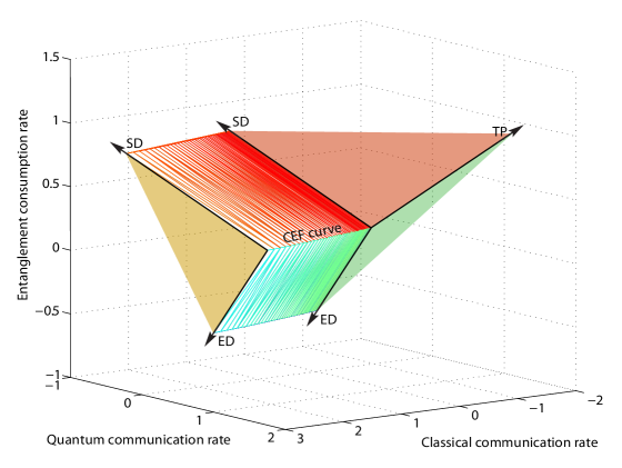
Figure 2: (Color online) A plot of the dynamic capacity region for a qubit dephasing channel with dephasing parameter $p=0.2$. The plot shows that the classically-enhanced father (CEF) trade-off curve lies along the boundary of the dynamic capacity region. The rest of the region is simply the combination of the CEF points with the unit protocols teleportation (TP), super-dense coding (SD), and entanglement distribution (ED).

The proof of the following theorem exploits the same techniques as in Ref. BHTW10 .

Theorem 9.1

The dynamic capacity region $\mathcal{C}_{\text{CQE}}(\Delta_{p})$ of a dephasing channel with dephasing parameter $p$ is the set of all $C$, $Q$, and $E$ such that

$$C+2Q \leq 1+H_{2}\left(\nu\right)-H_{2}(\gamma\left(\nu,p\right)),$$ (26)

$$Q+E \leq H_{2}\left(\nu\right)-H_{2}(\gamma\left(\nu,p\right)),$$ (27)

$$C+Q+E \leq 1-H_{2}(\gamma\left(\nu,p\right)),$$ (28)

where $\nu\in\left[0,1/2\right]$, $H_{2}$ is the binary entropy function, and

$$\gamma\left(\nu,p\right)\equiv\frac{1}{2}+\frac{1}{2}\sqrt{1-16\cdot\frac{p}{2}\left(1-\frac{p}{2}\right)\nu(1-\nu)}.$$

Proof

We first notice that it suffices to consider an ensemble of pure states whose reductions to $A^{\prime}$ are diagonal in the dephasing basis (as in Lemma 11 of Ref. BHTW10 ). Next we prove below that it is sufficient to consider an ensemble of the following form to characterize the boundary points of the region:

$$\frac{1}{2}\left|0\right\rangle\left\langle 0\right|^{X}\otimes\psi_{0}^{AA^{\prime}}+\frac{1}{2}\left|1\right\rangle\left\langle 1\right|^{X}\otimes\psi_{1}^{AA^{\prime}},$$ (29)

where $\psi_{0}^{AA^{\prime}}$ and $\psi_{1}^{AA^{\prime}}$ are pure states, defined as follows for $\nu\in\left[0,1/2\right]$:

$$\text{Tr}_{A}\left\{\psi_{0}^{AA^{\prime}}\right\} =\nu\left|0\right\rangle\left\langle 0\right|^{A^{\prime}}+\left(1-\nu\right)\left|1\right\rangle\left\langle 1\right|^{A^{\prime}},$$ (30)

$$\text{Tr}_{A}\left\{\psi_{1}^{AA^{\prime}}\right\} =\left(1-\nu\right)\left|0\right\rangle\left\langle 0\right|^{A^{\prime}}+\nu\left|1\right\rangle\left\langle 1\right|^{A^{\prime}}.$$ (31)

We now prove the above claim. We assume without loss of generality that the dephasing basis is the computational basis. Consider a classical-quantum state with a finite number $N$ of conditional density operators $\phi_{x}^{AA^{\prime}}$ whose reduction to $A^{\prime}$ is diagonal:

$$\rho^{XAA^{\prime}}\equiv\sum_{x=0}^{N-1}p_{X}\left(x\right)|x\rangle\langle x|^{X}\otimes\phi_{x}^{AA^{\prime}}.$$

We can form a new classical-quantum state with double the number of conditional density operators by “bit-flipping” the original conditional density operators:

$$\sigma^{XAA^{\prime}}\equiv\frac{1}{2}\sum_{x=0}^{N-1}p_{X}\left(x\right)\left(|x\rangle\langle x|^{X}\otimes\phi_{x}^{AA^{\prime}}+|x+N\rangle\langle x+N|^{X}\otimes X^{A^{\prime}}\phi_{x}^{AA^{\prime}}X^{A^{\prime}}\right),$$

where $X$ is the $\sigma_{X}$ “bit-flip” Pauli operator. Consider the following chain of inequalities that holds for all $\lambda,\mu\geq 0$:

$$I\left(AX;B\right)_{\rho}+\lambda I\left(A\rangle BX\right)_{\rho}+\mu\left(I\left(X;B\right)_{\rho}+I\left(A\rangle BX\right)_{\rho}\right)$$

$$=H\left(A|X\right)_{\rho}+\left(\mu+1\right)H\left(B\right)_{\rho}+\lambda H\left(B|X\right)_{\rho}-\left(\lambda+\mu+1\right)H\left(E|X\right)_{\rho}$$

$$\leq\left(\mu+1\right)H\left(B\right)_{\sigma}+H\left(A|X\right)_{\sigma}+\lambda H\left(B|X\right)_{\sigma}-\left(\lambda+\mu+1\right)H\left(E|X\right)_{\sigma}$$

$$=\left(\mu+1\right)+H\left(A|X\right)_{\sigma}+\lambda H\left(B|X\right)_{\sigma}-\left(\lambda+\mu+1\right)H\left(E|X\right)_{\sigma}$$

$$=\left(\mu+1\right)+\sum_{x}p_{X}\left(x\right)\left[H\left(A\right)_{\phi_{x}}+\lambda H\left(B\right)_{\phi_{x}}-\left(\lambda+\mu+1\right)H\left(E\right)_{\phi_{x}}\right]$$

$$\leq\left(\mu+1\right)+\max_{x}\left[H\left(A\right)_{\phi_{x}}+\lambda H\left(B\right)_{\phi_{x}}-\left(\lambda+\mu+1\right)H\left(E\right)_{\phi_{x}}\right]$$

$$=\left(\mu+1\right)+H\left(A\right)_{\phi_{x}^{\ast}}+\lambda H\left(B\right)_{\phi_{x}^{\ast}}-\left(\lambda+\mu+1\right)H\left(E\right)_{\phi_{x}^{\ast}}.$$

The first equality follows by standard entropic manipulations. The second equality follows because the conditional entropy $H\left(B|X\right)$ is invariant under a bit-flipping unitary on the input state that commutes with the channel: $H(B)_{X\rho_{x}^{B}X}=H(B)_{\rho_{x}^{B}}$. Furthermore, a bit flip on the input state does not change the eigenvalues for the output of the dephasing channel’s complementary channel: $H(E)_{\mathcal{N}^{c}(X\rho_{x}^{A^{\prime}}X)}=H(E)_{\mathcal{N}^{c}(\rho_{x}^{A^{\prime}})}$. The first inequality follows because entropy is concave, i.e., the local state $\sigma^{B}$ is a mixed version of $\rho^{B}$. The third equality follows because $H(B)_{\sigma^{B}}=H\left(\sum_{x}\frac{1}{2}p_{X}\left(x\right)(\rho_{x}^{B}+X\rho_{x}^{B}X)\right)=H\left(\frac{1}{2}\sum_{x}p_{X}\left(x\right)I\right)=1$. The fourth equality follows because the system $X$ is classical. The second inequality follows because the maximum value of a realization of a random variable is not less than its expectation. The final equality simply follows by defining $\phi_{x}^{\ast}$ to be the conditional density operator on systems $A$, $B$, and $E$ that arises from sending through the channel a state whose reduction to $A^{\prime}$ is of the form $\nu\left|0\right\rangle\left\langle 0\right|^{A^{\prime}}+\left(1-\nu\right)\left|1\right\rangle\left\langle 1\right|^{A^{\prime}}$. Thus, an ensemble of the kind in (29) is sufficient to attain a point on the boundary of the region.

Evaluating the entropic quantities in Theorem 4.1 on a state of the above form then gives the expression for the region in Theorem 9.1.

10 Single-letter dynamic capacity region for the quantum erasure channels

Below we show that the regularization in (8) is not necessary if the quantum channel is a quantum erasure channel. The quantum erasure channel also has a special structure, but the proof proceeds differently from that for a quantum Hadamard channel.

A quantum erasure channel with erasure parameter $\epsilon$ is the following map GBP97 :

$$\mathcal{N}_{\epsilon}\left(\rho\right)\equiv\left(1-\epsilon\right)\rho+\epsilon\left|e\right\rangle\left\langle e\right|.$$

Notice that the receiver can perform a measurement $\left\{\left|0\right\rangle\left\langle 0\right|+\left|1\right\rangle\left\langle 1\right|,\left|e\right\rangle\left\langle e\right|\right\}$ and can learn whether the channel erased the state. The receiver can do this without disturbing the state in any way. An isometric extension $U_{\mathcal{N}_{\epsilon}}^{A^{\prime}\rightarrow BE}$ of it acts as follows on a purification $\left|\psi\right\rangle^{AA^{\prime}}$ of the state $\rho^{A^{\prime}}$:

$$U_{\mathcal{N}_{\epsilon}}^{A^{\prime}\rightarrow BE}\left|\psi\right\rangle^{AA^{\prime}}=\sqrt{1-\epsilon}\left|\psi\right\rangle^{AB}\left|e\right\rangle^{E}+\sqrt{\epsilon}\left|\psi\right\rangle^{AE}\left|e\right\rangle^{B}.$$

In the above representation, we see that the erasure channel has the interpretation that it hands the input to Bob with probability $1-\epsilon$ while giving an erasure flag $\left|e\right\rangle$ to Eve, and it hands the input to Eve with probability $\epsilon$ while giving the erasure flag to Bob.

Theorem 10.1

The dynamic capacity region $\mathcal{C}_{\mathrm{{CQE}}}(\mathcal{N}_{\epsilon})$ of a quantum erasure channel $\mathcal{N}_{\epsilon}$ is the set of all $C$, $Q$, and $E$ such that

$$C+2Q \leq\left(1-\epsilon\right)\left(1+H_{2}\left(p\right)\right),$$

$$Q+E \leq\left(1-2\epsilon\right)H_{2}\left(p\right),$$

$$C+Q+E \leq 1-\epsilon-\epsilon H_{2}\left(p\right),$$

where $p\in\left[0,1/2\right]$.

Figure 3 plots the dynamic capacity region of a quantum erasure channel with erasure parameter $\epsilon=1/4$. It turns out that time-sharing is the optimal strategy here, and there is not an interesting trade-off curve for the quantum erasure channel.

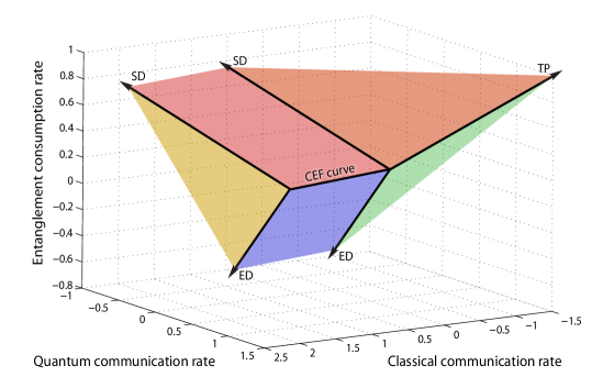
Figure 3: (Color online) A plot of the dynamic capacity region for a qubit erasure channel with erasure parameter $\epsilon=1/4$. The plot shows that the classically-enhanced father (CEF) trade-off curve lies along the boundary of the dynamic capacity region and it is not actually a curve but rather a line because time-sharing is optimal. The rest of the region is simply the combination of the CEF points with the unit protocols teleportation (TP), super-dense coding (SD), and entanglement distribution (ED).

We in fact proved Theorem 10.1 in Ref. HW09T3  by employing a reductio ad absurdum argument reminiscent of the earliest arguments for proving capacities of quantum erasure channels PhysRevLett.78.3217 . This approach gives the correct answer, but suffers from two shortcomings:

1. We do not learn much about how to exploit the structure of the quantum erasure channel with the reductio ad absurdum approach. As an example, Smith and Yard exploited the simple structure of the quantum erasure channel and discovered far reaching consequences SY08 . In particular, they discovered that the quantum capacity (and for that matter, any future proposed quantum capacity formula) can never be generally additive, by combining the erasure channel with another one.

2. The reductio ad absurdum argument rests on the assumption that several known capacity formulas are continuous as a function of channels. Leung and Smith later showed that the known formulas are indeed continuous LS08 , redeeming the original argument in Ref. PhysRevLett.78.3217 .

Here, we prove Theorem 10.1 above by carefully studying the structure of the quantum erasure channel and its additivity properties for the full dynamic capacity region. We prove the theorem in a few steps. First, we prove that the classical capacity of the quantum erasure channel admits a single-letter formula. We then simplify the quantum dynamic capacity formula in (21) for the case of a quantum erasure channel and find that it is only necessary to consider certain values of the parameters $\mu$ and $\lambda$ when we optimize. The proof of Lemma 7 exploits these conditions to show that the quantum dynamic capacity formula is additive for the case of two quantum erasure channels. It then follows by a trivial induction step (the same as in Lemma 1) that the full dynamic region single-letterizes and is of the form in Theorem 10.1.

Lemma 3 (Bennett et al. PhysRevLett.78.3217 )

The Holevo information of a quantum erasure channel is equal to $1-\epsilon$:

$$\chi\left(\mathcal{N}_{\epsilon}\right)\equiv\max_{\sigma^{XB}}I\left(X;B\right)=1-\epsilon$$

Proof

We begin with an input ensemble of the following form:

$$\rho^{XA^{\prime}}\equiv\sum_{x}p_{X}\left(x\right)\left|x\right\rangle\left\langle x\right|^{X}\otimes\phi_{x}^{A^{\prime}},$$

where the states $\phi_{x}^{A^{\prime}}$ are pure (it suffices to consider pure state ensembles for classical capacity). Feeding the $A^{\prime}$ system into the quantum erasure channel leads to a classical-quantum state $\sigma^{XB}=\sum_{x}p_{X}\left(x\right)\left|x\right\rangle\left\langle x\right|^{X}\otimes\mathcal{N}_{\epsilon}^{A^{\prime}\to B}(\phi_{x}^{A^{\prime}})$. Bob can then measure his system $B$ to learn whether the channel erases the qubit. Let $X_{E}$ denote a classical register where Bob places the result of the measurement so that we then have the state $\sigma^{XBX_{E}}$. It holds that any entropy evaluated on system $B$ is equal to the joint entropy of $B$ and $X_{E}$ because this measurement does not disturb the state in any way. Consider the following chain of inequalities:

$$I\left(X;B\right)_{\sigma} =H\left(B\right)_{\sigma}-H\left(B|X\right)_{\sigma}$$

$$=H\left(BX_{E}\right)_{\sigma}-H\left(BX_{E}|X\right)_{\sigma}$$

$$=H\left(B|X_{E}\right)_{\sigma}-H\left(B|X_{E}X\right)_{\sigma}$$

$$=\left(1-\epsilon\right)H\left(A^{\prime}\right)_{\rho}-\left(1-\epsilon\right)H\left(A^{\prime}|X\right)_{\rho}$$

$$=\left(1-\epsilon\right)I\left(X;A^{\prime}\right)_{\rho}$$

$$\leq\left(1-\epsilon\right).$$

The first equality follows by expanding the mutual information and the second equality follows from the above fact regarding the joint entropy of $B$ and $X_{E}$. The third equality follows by expanding and canceling terms. The fourth equality follows by conditioning on the classical erasure flag register $X_{E}$ and realizing that the entropy of Bob’s system $B$ is the entropy of the input state with probability $1-\epsilon$ and otherwise is the entropy of the erasure state $\left|e\right\rangle$ (this latter entropy vanishes because this state is pure). Thus, the above sequence of steps reduces an optimization problem on the output of the channel to a simple optimization over the input ensemble. The Holevo information is then $1-\epsilon$ because the quantity $I\left(X;A^{\prime}\right)_{\rho}$ can never be larger than unity for the case of a qubit erasure channel (it reaches unity for an ensemble of two orthogonal pure states chosen with equal probability).

Lemma 4

The following additivity lemma holds for a quantum erasure channel $\mathcal{N}_{\epsilon}$:

$$\chi\left(\mathcal{N}_{\epsilon}\otimes\mathcal{N}_{\epsilon}\right)=\chi\left(\mathcal{N}_{\epsilon}\right)+\chi\left(\mathcal{N}_{\epsilon}\right)=2\left(1-\epsilon\right).$$

Proof

It suffices to prove the inequality $\chi\left(\mathcal{N}_{\epsilon}\otimes\mathcal{N}_{\epsilon}\right)\leq\chi\left(\mathcal{N}_{\epsilon}\right)+\chi\left(\mathcal{N}_{\epsilon}\right)$ because the other inequality holds trivially. We define the following ensemble of states for the tensor product channel $\mathcal{N}_{\epsilon}\otimes\mathcal{N}_{\epsilon}$:

$$\rho^{XA_{1}^{\prime}A_{2}^{\prime}}\equiv\sum_{x}p_{X}\left(x\right)\left|x\right\rangle\left\langle x\right|^{X}\otimes\phi_{x}^{A_{1}^{\prime}A_{2}^{\prime}}.$$ (32)

We can also define the following augmented ensemble based on the above one:

$$\sigma^{XIJA_{1}^{\prime}A_{2}^{\prime}}\equiv\frac{1}{16}\sum_{x,i,j}p_{X}\left(x\right)\left|x\right\rangle\left\langle x\right|^{X}\otimes\left|i\right\rangle\left\langle i\right|^{I}\otimes\left|j\right\rangle\left\langle j\right|^{J}\otimes(\sigma_{i}^{A_{1}^{\prime}}\otimes\sigma_{j}^{A_{2}^{\prime}})\phi_{x}^{A_{1}^{\prime}A_{2}^{\prime}}(\sigma_{i}^{A_{1}^{\prime}}\otimes\sigma_{j}^{A_{2}^{\prime}}),$$ (33)

where $\sigma_{0}\equiv I$, $\sigma_{1}\equiv\sigma_{X}$, $\sigma_{2}\equiv\sigma_{Y}$, and $\sigma_{3}\equiv\sigma_{Z}$. In particular, note that we obtain the maximally mixed state when tracing over classical registers $I$ and $J$. Let $\omega^{XB_{1}B_{2}}$ and $\theta^{XIJB_{1}B_{2}}$ denote the states obtained by sending systems $A_{1}^{\prime}$ and $A_{2}^{\prime}$ of the respective states $\rho^{XA_{1}^{\prime}A_{2}^{\prime}}$ and $\sigma^{XIJA_{1}^{\prime}A_{2}^{\prime}}$ through two uses of the quantum erasure channel. Let $X_{E,1}$ and $X_{E,2}$ denote the classical variables Bob obtains by determining whether the channel erased his states (they also denote the registers where he places the results). Consider the following chain of inequalities that holds for any state $\omega^{XB_{1}B_{2}}$:

$$I\left(X;B_{1}B_{2}\right)_{\omega} =H\left(B_{1}B_{2}\right)_{\omega}-H\left(B_{1}B_{2}|X\right)_{\omega}$$

$$=H\left(B_{1}B_{2}|X_{E,1}X_{E\,,2}\right)_{\omega}-H\left(B_{1}B_{2}|X_{E,1}X_{E\,,2}X\right)_{\omega}$$

$$=\left(1-\epsilon\right)^{2}H\left(A_{1}^{\prime}A_{2}^{\prime}\right)_{\rho}+\left(1-\epsilon\right)\epsilon\left(H\left(A_{1}^{\prime}\right)_{\rho}+H\left(A_{2}^{\prime}\right)_{\rho}\right)$$

$$\ \ \ \ \ \ -\left(1-\epsilon\right)^{2}H\left(A_{1}^{\prime}A_{2}^{\prime}|X\right)_{\rho}-\left(1-\epsilon\right)\epsilon\left(H\left(A_{1}^{\prime}|X\right)_{\rho}+H\left(A_{2}^{\prime}|X\right)_{\rho}\right)$$

$$\leq 2\left(1-\epsilon\right)-\left(1-\epsilon\right)^{2}H\left(A_{1}^{\prime}A_{2}^{\prime}|XIJ\right)_{\sigma}-\left(1-\epsilon\right)\epsilon\left(H\left(A_{1}^{\prime}|XIJ\right)_{\sigma}+H\left(A_{2}^{\prime}|XIJ\right)_{\sigma}\right)$$

$$\leq 2\left(1-\epsilon\right).$$

The first equality holds by expanding the mutual information. The next equality holds because an “erasure measurement” does not change entropy. The third equality follows by exploiting the properties of the erasure channels. The first inequality holds because the unconditional entropies of the $A^{\prime}$ systems on the state $\rho$ are always less than those for the state $\sigma$. The final inequality follows because the entropies in the previous line are non-negative. The statement of the theorem then follows.

Lemma 5

The quantum dynamic capacity formula in (21) simplifies as follows for a quantum erasure channel $\mathcal{N}_{\epsilon}$:

$$D_{\lambda,\mu}\left(\mathcal{N}_{\epsilon}\right)\equiv\max_{p\in\left[0,1/2\right]}\left(1-\epsilon\right)\left(1+H_{2}\left(p\right)\right)+\lambda\left(1-2\epsilon\right)H_{2}\left(p\right)+\mu\left(\left(1-\epsilon\right)-\epsilon H_{2}\left(p\right)\right).$$ (34)

Thus, the “one-letter” dynamic capacity region of a quantum erasure channel is as Theorem 10.1 states.

Proof

We exploit the following classical-quantum states:

$$\rho^{XAA^{\prime}} \equiv\sum_{x}p_{X}\left(x\right)\left|x\right\rangle\left\langle x\right|^{X}\otimes\phi_{x}^{AA^{\prime}},$$

$$\sigma^{XIAA^{\prime}} \equiv\sum_{x,i}\frac{1}{4}p_{X}\left(x\right)\left|x\right\rangle\left\langle x\right|^{X}\otimes\left|i\right\rangle\left\langle i\right|^{I}\otimes(\sigma_{i}^{A^{\prime}})\phi_{x}^{AA^{\prime}}(\sigma_{i}^{A^{\prime}}),$$

and let $\rho^{XABE}$ and $\sigma^{XIABE}$ be the states obtained by transmitting the $A^{\prime}$ system through the isometric extension of the erasure channel. Let $\sigma_{x}^{A^{\prime}}\equiv$Tr${}_{A}\left\{\phi_{x}^{AA^{\prime}}\right\}$. Furthermore, let the eigenvalues of the state $\sigma_{x}^{A^{\prime}}$ with highest entropy on system $A^{\prime}$ be $p$ and $1-p$. Consider that the following chain of inequalities holds for any state $\rho^{XABE}$:

$$I\left(AX;B\right)_{\rho}+\lambda I\left(A\rangle BX\right)_{\rho}+\mu\left(I\left(X;B\right)_{\rho}+I\left(A\rangle BX\right)_{\rho}\right)$$

$$=H\left(A|X\right)_{\rho}+\left(\mu+1\right)H\left(B\right)_{\rho}+\lambda H\left(B|X\right)_{\rho}-\left(\lambda+\mu+1\right)H\left(E|X\right)_{\rho}$$

$$=H\left(A^{\prime}|X\right)_{\rho}+\left(\mu+1\right)H\left(B|X_{E}\right)_{\rho}+\lambda H\left(B|X_{E}X\right)_{\rho}-\left(\lambda+\mu+1\right)H\left(E|X_{E}X\right)_{\rho}$$

$$=H\left(A^{\prime}|X\right)_{\rho}+\left(\mu+1\right)\left(1-\epsilon\right)H\left(A^{\prime}\right)_{\rho}+\lambda\left(1-\epsilon\right)H\left(A^{\prime}|X\right)_{\rho}-\left(\lambda+\mu+1\right)\epsilon H\left(A^{\prime}|X\right)_{\rho}$$

$$\leq\left(\mu+1\right)\left(1-\epsilon\right)+\left(1+\lambda\left(1-\epsilon\right)-\left(\lambda+\mu+1\right)\epsilon\right)H\left(A^{\prime}|XI\right)_{\sigma}$$

$$=\left(\mu+1\right)\left(1-\epsilon\right)+\left(1-\epsilon+\lambda\left(1-2\epsilon\right)-\mu\epsilon\right)\sum_{x}p_{X}\left(x\right)H\left(A^{\prime}\right)_{\sigma_{x}}$$

$$\leq\left(\mu+1\right)\left(1-\epsilon\right)+\left(1-\epsilon+\lambda\left(1-2\epsilon\right)-\mu\epsilon\right)H\left(A^{\prime}\right)_{\sigma_{x}^{\ast}}$$

$$=\left(1-\epsilon\right)\left(1+H_{2}\left(p\right)\right)+\mu\left(1-\epsilon-\epsilon H_{2}\left(p\right)\right)+\lambda\left(1-2\epsilon\right)H_{2}\left(p\right).$$

The first equality follows by standard entropic manipulations. The second equality follows by incorporating the classical erasure flag variable. The third equality follows by exploiting the properties of the quantum erasure channel. The first inequality follows because the unconditional entropy of the state $\rho$ is always less than that of the state $\sigma$. The next equality follows by expanding the conditional entropy. The second inequality follows because an average is always less than a maximum. The final equality follows by plugging in the eigenvalues of $\sigma_{x}^{\ast}$. The form of the quantum dynamic capacity formula then follows because this chain of inequalities holds for any input ensemble.

Lemma 6

It suffices to consider the set of $\lambda,\mu\geq 0$ for which

$$\left(1-\epsilon\right)+\lambda\left(1-2\epsilon\right)\geq\mu\epsilon.$$

Otherwise, we are just maximizing the classical capacity, which we know from Lemma 3 is equal to $1-\epsilon$.

Proof

Consider rewriting the expression in (34) as follows:

$$\max_{p\in\left[0,1/2\right]}\left(1-\epsilon\right)+\mu\left(1-\epsilon\right)+\left[\left(1-\epsilon\right)+\lambda\left(1-2\epsilon\right)-\mu\epsilon\right]H_{2}\left(p\right).$$

Suppose that the expression in square brackets is negative, i.e.,

$$\left(1-\epsilon\right)+\lambda\left(1-2\epsilon\right)<\mu\epsilon.$$

Then the maximization over $p$ simply chooses $p=0$ so that $H_{2}\left(p\right)$ vanishes and the negative term disappears. The resulting expression for the quantum dynamic capacity formula is

$$\left(1-\epsilon\right)+\mu\left(1-\epsilon\right),$$

which corresponds to the following region

$$C+2Q \leq 1-\epsilon,$$

$$Q+E \leq 0,$$

$$C+Q+E \leq 1-\epsilon.$$

The above region is equivalent to a translation of the unit resource capacity region to the classical capacity rate triple $\left(1-\epsilon,0,0\right)$. Thus, it suffices to restrict the parameters $\lambda$ and $\mu$ as above for the quantum erasure channel.

Lemma 7

The following additivity relation holds for two quantum erasure channels $\mathcal{N}_{\epsilon}$ with the same erasure parameter $\epsilon$:

$$D_{\lambda,\mu}(\mathcal{N}_{\epsilon}\otimes\mathcal{N}_{\epsilon})=D_{\lambda,\mu}(\mathcal{N}_{\epsilon})+D_{\lambda,\mu}(\mathcal{N}_{\epsilon}).$$

Proof

We prove the non-trivial inequality $D_{\lambda,\mu}(\mathcal{N}_{\epsilon}\otimes\mathcal{N}_{\epsilon})\leq D_{\lambda,\mu}(\mathcal{N}_{\epsilon})+D_{\lambda,\mu}(\mathcal{N}_{\epsilon})$. We define the following states:

$$\rho^{XAA_{1}^{\prime}A_{2}^{\prime}} \equiv\sum_{x}p_{X}\left(x\right)\left|x\right\rangle\left\langle x\right|^{X}\otimes\phi_{x}^{AA_{1}^{\prime}A_{2}^{\prime}},$$

$$\omega^{XAB_{1}E_{1}B_{2}E_{2}} \equiv U_{\mathcal{N}_{\epsilon}}^{A_{1}^{\prime}\rightarrow B_{1}E_{1}}\otimes U_{\mathcal{N}_{\epsilon}}^{A_{2}^{\prime}\rightarrow B_{2}E_{2}}(\rho^{XAA_{1}^{\prime}A_{2}^{\prime}}),$$

and we suppose that $\rho^{XAA_{1}A_{2}}$ is the state that maximizes $D_{\lambda,\mu}(\mathcal{N}_{\epsilon}\otimes\mathcal{N}_{\epsilon})$. Consider the following equality:

$$I\left(AX;B_{1}B_{2}\right)_{\omega}+\lambda I\left(A\rangle B_{1}B_{2}X\right)_{\omega}+\mu\left(I\left(X;B_{1}B_{2}\right)_{\omega}+I\left(A\rangle B_{1}B_{2}X\right)_{\omega}\right)$$

$$=H\left(A|X\right)_{\omega}+H\left(B_{1}B_{2}\right)_{\omega}-H\left(E_{1}E_{2}|X\right)_{\omega}+\lambda\left(H\left(B_{1}B_{2}|X\right)_{\omega}-H\left(E_{1}E_{2}|X\right)_{\omega}\right)$$

$$\ \ \ \ \ \ \ \ +\mu\left(H\left(B_{1}B_{2}\right)_{\omega}-H\left(E_{1}E_{2}|X\right)_{\omega}\right).$$

It follows simply by rewriting entropies. We continue below:

$$=H\left(A_{1}^{\prime}A_{2}^{\prime}|X\right)_{\rho}+\left(1-\epsilon\right)^{2}H\left(A_{1}^{\prime}A_{2}^{\prime}\right)_{\rho}+\epsilon\left(1-\epsilon\right)\left(H\left(A_{1}^{\prime}\right)_{\rho}+H\left(A_{2}^{\prime}\right)_{\rho}\right)$$

$$\ \ \ \ \ \ -\left[\epsilon^{2}H\left(A_{1}^{\prime}A_{2}^{\prime}|X\right)_{\rho}+\epsilon\left(1-\epsilon\right)\left(H\left(A_{1}^{\prime}|X\right)_{\rho}+H\left(A_{2}^{\prime}|X\right)_{\rho}\right)\right]$$

$$\ \ \ \ \ \ +\lambda\left[\left(1-\epsilon\right)^{2}H\left(A_{1}^{\prime}A_{2}^{\prime}|X\right)_{\rho}+\epsilon\left(1-\epsilon\right)\left(H\left(A_{1}^{\prime}|X\right)_{\rho}+H\left(A_{2}^{\prime}|X\right)_{\rho}\right)\right]$$

$$\ \ \ \ \ \ -\lambda\left[\epsilon^{2}H\left(A_{1}^{\prime}A_{2}^{\prime}|X\right)_{\rho}+\epsilon\left(1-\epsilon\right)\left(H\left(A_{1}^{\prime}|X\right)_{\rho}+H\left(A_{2}^{\prime}|X\right)_{\rho}\right)\right]$$

$$\ \ \ \ \ \ +\mu\left[\left(1-\epsilon\right)^{2}H\left(A_{1}^{\prime}A_{2}^{\prime}\right)_{\rho}+\epsilon\left(1-\epsilon\right)\left(H\left(A_{1}^{\prime}\right)_{\rho}+H\left(A_{2}^{\prime}\right)_{\rho}\right)\right]$$

$$\ \ \ \ \ \ -\mu\left[\epsilon^{2}H\left(A_{1}^{\prime}A_{2}^{\prime}|X\right)_{\rho}+\epsilon\left(1-\epsilon\right)\left(H\left(A_{1}^{\prime}|X\right)_{\rho}+H\left(A_{2}^{\prime}|X\right)_{\rho}\right)\right].$$

The above equality follows by exploiting the properties of the quantum erasure channel. Continuing, the above quantity is less than the following one:

$$\leq 2\left(1-\epsilon\right)+\left(1-\epsilon^{2}\right)H\left(A_{1}^{\prime}A_{2}^{\prime}|XIJ\right)_{\sigma}+\epsilon\left(1-\epsilon\right)\left(H\left(A_{1}^{\prime}|XIJ\right)_{\sigma}+H\left(A_{2}^{\prime}|XIJ\right)_{\sigma}\right)$$

$$\ \ \ \ \ \ +\lambda\left(1-2\epsilon\right)H\left(A_{1}^{\prime}A_{2}^{\prime}|XIJ\right)_{\sigma}$$

$$\ \ \ \ \ \ +\mu\left[2\left(1-\epsilon\right)-\epsilon^{2}H\left(A_{1}^{\prime}A_{2}^{\prime}|XIJ\right)_{\sigma}-\epsilon\left(1-\epsilon\right)\left(H\left(A_{1}^{\prime}|XIJ\right)_{\sigma}-H\left(A_{2}^{\prime}|XIJ\right)_{\sigma}\right)\right]$$

$$=2\left(1-\epsilon\right)+\left(1-\epsilon\right)\left(H\left(A_{1}^{\prime}|XIJ\right)_{\sigma}+H\left(A_{2}^{\prime}|XIJ\right)_{\sigma}\right)+\lambda\left(1-2\epsilon\right)\left(H\left(A_{1}^{\prime}|XIJ\right)_{\sigma}+H\left(A_{2}^{\prime}|XIJ\right)_{\sigma}\right)$$

$$\ \ \ \ \ \ +\mu\left[2\left(1-\epsilon\right)-\epsilon\left(H\left(A_{1}^{\prime}|XIJ\right)_{\sigma}-H\left(A_{2}^{\prime}|XIJ\right)_{\sigma}\right)\right]$$

$$\ \ \ \ \ \ -\left[\left(1-\epsilon^{2}+\lambda\left(1-2\epsilon\right)-\mu\epsilon^{2}\right)I\left(A_{1}^{\prime};A_{2}^{\prime}|XIJ\right)_{\sigma}\right]$$

$$\leq D_{\lambda,\mu}\left(\mathcal{N}_{\epsilon}\right)+D_{\lambda,\mu}\left(\mathcal{N}_{\epsilon}\right)-\left[\left(1-\epsilon^{2}+\lambda\left(1-2\epsilon\right)-\mu\epsilon^{2}\right)I\left(A_{1}^{\prime};A_{2}^{\prime}|XIJ\right)_{\rho}\right]$$

$$\leq D_{\lambda,\mu}\left(\mathcal{N}_{\epsilon}\right)+D_{\lambda,\mu}\left(\mathcal{N}_{\epsilon}\right).$$

The first inequality follows from similar proofs we have seen for a state $\sigma$ of the form in (33). The first equality follows by rearranging terms. The second inequality follows from the form of $D_{\lambda,\mu}$ in (34). The final inequality follows because Lemma 6 states that it is sufficient to consider $\left(1-\epsilon\right)+\lambda\left(1-2\epsilon\right)\geq\mu\epsilon$. Note that this condition implies that

$$1-\epsilon^{2}+\lambda\left(1-2\epsilon\right)\geq\mu\epsilon^{2},$$

and hence that the quantity in square brackets in the line above the last one is positive.

11 Conclusion

We found a purely information theoretic approach to proving the converse part of the dynamic capacity region. This technique should be simpler to understand for those unfamiliar with the quantum Shannon theory literature. We also phrased the optimization task for the full dynamic capacity region in terms of the quantum dynamic capacity formula in (21) and proved its additivity (and hence single-letterization of the dynamic capacity region) for the quantum Hadamard channels and quantum erasure channels. We note some open problems below.

There might be room for improvement in our formulas that characterize the dynamic capacity region when the channel is not of the Hadamard class or a quantum erasure channel. Though, our characterization has the simple interpretation as the regularization of what one can achieve with the classically-enhanced father protocol HW08GFP  combined with teleportation, super-dense coding, and entanglement distribution. It is difficult to imagine a simpler characterization than this one, despite its multi-letter nature for the general case.

We would like to find other channels besides the Hadamard or erasure channels for which the region single-letterizes. We conjecture that additivity of the quantum dynamic capacity formula in (21) holds for channels that have hybrid Hadamard-erasure behavior such as the phase erasure channel in Ref. PhysRevLett.78.3217 . It would also be interesting to find channels that are not hybrid Hadamard-erasure for which additivity of (21) holds.

There is also one interesting speculation to muse over that Professor David Avis suggested to us. Do each of the inequalities in Theorem 4.1 correspond to some fundamental physical law? This might shed further connections between information theory and physics that have not been elucidated yet.

References

- (1) Robert Alicki and Mark Fannes. Continuity of quantum conditional information. Journal of Physics A: Mathematical and General, 37(5):L55–L57, 2004.
- (2) Howard Barnum, Emanuel Knill, and Michael A. Nielsen. On quantum fidelities and channel capacities. IEEE Transactions on Information Theory, 46:1317–1329, 2000.
- (3) Charles H. Bennett, Gilles Brassard, Claude Crépeau, Richard Jozsa, Asher Peres, and William K. Wootters. Teleporting an unknown quantum state via dual classical and Einstein-Podolsky-Rosen channels. Physical Review Letters, 70:1895–1899, 1993.
- (4) Charles H. Bennett, David P. DiVincenzo, and John A. Smolin. Capacities of quantum erasure channels. Physical Review Letters, 78(16):3217–3220, April 1997.
- (5) Charles H. Bennett, Peter W. Shor, John A. Smolin, and Ashish V. Thapliyal. Entanglement-assisted capacity of a quantum channel and the reverse Shannon theorem. IEEE Transactions on Information Theory, 48:2637, 2002.
- (6) Charles H. Bennett and Stephen J. Wiesner. Communication via one- and two-particle operators on Einstein-Podolsky-Rosen states. Physical Review Letters, 69:2881–2884, 1992.
- (7) Stephen Boyd and Lieven Vandenberghe. Convex Optimization. Cambridge University Press, The Edinburgh Building, Cambridge, CB2 8RU, UK, 2004.
- (8) Kamil Brádler. An infinite sequence of additive channels: the classical capacity of cloning channels. IEEE Transactions on Information Theory, 57(8):5497–5503, August 2011. arXiv:0903.1638.
- (9) Kamil Brádler, Patrick Hayden, Dave Touchette, and Mark M. Wilde. Trade-off capacities of the quantum Hadamard channels. Physical Review A, 81:062312, June 2010. arXiv:1001.1732.
- (10) Igor Devetak. The private classical capacity and quantum capacity of a quantum channel. IEEE Transactions on Information Theory, 51(1):44–55, 2005.
- (11) Igor Devetak, Aram W. Harrow, and Andreas Winter. A resource framework for quantum Shannon theory. IEEE Transactions on Information Theory, 54(10):4587–4618, October 2008.
- (12) Igor Devetak and Peter W. Shor. The capacity of a quantum channel for simultaneous transmission of classical and quantum information. Communications in Mathematical Physics, 256(2):287–303, 2005.
- (13) M. Grassl, Th. Beth, and T. Pellizzari. Codes for the quantum erasure channel. Physical Review A, 56(1):33–38, July 1997.
- (14) Alexander S. Holevo. The capacity of the quantum channel with general signal states. IEEE Transactions on Information Theory, 44:269–273, 1998.
- (15) Min-Hsiu Hsieh and Mark M. Wilde. Theory of Quantum Computation, Communication, and Cryptography, volume 5906 of Lecture Notes in Computer Science, chapter Optimal Trading of Classical Communication, Quantum Communication, and Entanglement, pages 85–93. Springer-Verlag, May 2009.
- (16) Min-Hsiu Hsieh and Mark M. Wilde. Entanglement-assisted communication of classical and quantum information. IEEE Transactions on Information Theory, 56(9):4682–4704, September 2010. arXiv:0811.4227.
- (17) Min-Hsiu Hsieh and Mark M. Wilde. Trading classical communication, quantum communication, and entanglement in quantum Shannon theory. IEEE Transactions on Information Theory, 56(9):4705–4730, September 2010. arXiv:0901.3038.
- (18) Christopher King, Keiji Matsumoto, Michael Nathanson, and Mary Beth Ruskai. Properties of conjugate channels with applications to additivity and multiplicativity. Markov Processes and Related Fields, 13(2):391–423, 2007. J. T. Lewis memorial issue.
- (19) Debbie Leung and Graeme Smith. Continuity of quantum channel capacities. Communications in Mathematical Physics, 292(1):201–215, November 2009.
- (20) Elliot H. Lieb and Mary Beth Ruskai. Proof of strong subadditivity of quantum-mechanical entropy. Journal of Mathematical Physics, 14:1938, 1973.
- (21) Seth Lloyd. The capacity of a noisy quantum channel. Physical Review A, 55:1613–1622, 1997.
- (22) Michael A. Nielsen and Isaac L. Chuang. Quantum Computation and Quantum Information. Cambridge University Press, New York, 2000.
- (23) Benjamin Schumacher and Michael A. Nielsen. Quantum data processing and error correction. Physical Review A, 54:2629–2635, 1996.
- (24) Benjamin Schumacher and Michael D. Westmoreland. Sending classical information via noisy quantum channels. Physical Review A, 56:131–138, 1997.
- (25) Peter W. Shor. The quantum channel capacity and coherent information. MSRI workshop on quantum computation, 2002.
- (26) Graeme Smith and Jon Yard. Quantum communication with zero-capacity channels. Science, 321:1812–1815, September 2008.
- (27) Jon Yard. Simultaneous classical-quantum capacities of quantum multiple access channels. PhD thesis, Stanford University, Stanford, CA, 2005. quant-ph/0506050.