Exploratory Analysis of Functional Data via Clustering and Optimal Segmentation

Abstract

We propose in this paper an exploratory analysis algorithm for functional data. The method partitions a set of functions into $K$ clusters and represents each cluster by a simple prototype (e.g., piecewise constant). The total number of segments in the prototypes, $P$, is chosen by the user and optimally distributed among the clusters via two dynamic programming algorithms. The practical relevance of the method is shown on two real world datasets.

1 Introduction

Functional Data Analysis [26] addresses problems in which the observations are described by functions rather than finite dimensional vectors. A well known real world example of such data is given by spectrometry in which each object is analysed via one spectrum, that is a function which maps wavelengths to absorbance values. Online monitoring of hardware is also a good example of such data: each object is described by several time series associated to physical quantities monitored at specified sampling rates.

Another application domain is related to electric power consumption curves, also called (electric) load curves. Such data describes the electric power consumption over time of one household or one small or large industry. Load curves can be very voluminous since there are many consumers (over 35 millions in France) which can be observed during a long period (often several years) and at a rate up to one point every minute. Consequently, there is a strong need for applying unsupervised learning methods to summarize such datasets of load curves. A typical way to do so is to split each curve into daily (or weekly) periods and perform a clustering of such daily curves. The motivation of such analyses is related to several practical problems: understanding the consumption behaviour of consumers in relation to their equipment or weather conditions, defining new prices, optimizing the production of electric power, and in the next years monitoring the household consumption to face high peaks.

We focus in this paper on the exploratory analysis of a set of curves (or time series). The main idea is to provide the analyst with a summary of the set with a manageable complexity. A classical solution for multivariate data consists in using a prototype based clustering approach: each cluster is summarized by its prototype. Standard clustering methods such as K means and Self Organizing Map have been adapted to functional data and could be used to implement this solution [1, 6, 8, 29]. Another possibility comes from the symbolization approaches in which a time series is represented by a sequence of symbols. In the SAX approach [24], the time series is transformed into a piecewise representation with contiguous time intervals of equal size: the value associated with each interval is the average of actual values in the interval. This approach is very fast but does not give any guarantee on the associated error. In [15], a piecewise constant approximation of a time series is constructed via a segmentation of the time domain into contiguous intervals on which the series is represented by its average value, which can be turned into a label in a subsequent quantization step. When we are given a set of curves, an unique segmentation can be found in order to represent all the curves on a common piecewise constant basis (see [28] for an optimal solution). This was used as a preprocessing step in e.g. [30, 19].

We propose in this paper to merge the two approaches: we build a K means like clustering of a set of functions in which each prototype is given by a simple function defined in a piecewise way. The input interval of each prototype is partitioned into sub-intervals (segments) on which the prototype assumes a simple form (e.g., constant). Using dynamic programming, we obtain an optimal segmentation for each prototype while the number of segments used in each cluster is also optimally chosen with respect to a user specified total number segments. In the case of piecewise constant prototypes, a set of functions is summarized via $2P-K$ real values, where $K$ is the number of prototypes and $P$ the total number of segments used to represent the prototypes.

The rest of this paper is organized as follows. Section 2 introduces the problem of finding a simple summary of a single function, links this problem with optimal segmentation and provides an overview of the dynamic programming solution to optimal segmentation. Section 3 shows how single function summarizing methods can be combined to clustering methods to give a summary of a set of functions. It also introduces the optimal resource allocation algorithm that computes an optimal number of segments for each cluster. Section 4 illustrates the method on two real world datasets.

2 Summarizing one function via optimal segmentation: a state-of-the-art

The proposed solution is built on two elements that are mostly independent: any standard clustering algorithm that can handle functional data and a functional summarizing technique that can build an appropriate low complexity representation of a set of homogeneous functions. The present section describes the summarizing technique for a single function; the extension to a set of functions is described in Section 3.

Building a summary of a function is deeply connected to building an optimal segmentation of the function, a problem which belongs to the general task of function approximation. Optimal segmentation has been studied under different point of views (and different names) in a large and scattered literature (see [32, 3, 21, 22, 25, 2, 16] and references therein). The goal of the present section is not to provide new material but rather to give a detailed exposition of the relations between summary and segmentation on the one hand, and of the optimal segmentation framework itself on the other hand.

2.1 Simple functions

We consider a function $s$ sampled in $M$ distinct points $(t_{k})_{k=1}^{M}$ from the interval $[t_{1},t_{M}]$ (points are assumed to be ordered, i.e., $t_{1}<t_{2}<\ldots<t_{M}$). Our goal is to approximate $s$ by a simpler function $g$ on $[t_{1},t_{M}]$. The simplicity concept targeted in this article is not based on smoothness as in regularization [33] or on capacity as in learning theory (see e.g., [9]). It corresponds rather to an informal measure of the simplicity of the visual representation of $g$ for a human analyst.

The difference between those three aspects (smoothness, capacity and visual simplicity) can be illustrated by an elementary example: let us assume that $g$ is chosen as a linear combination of $N$ fixed functions, i.e.,

$$g(t)=\sum_{i=1}^{N}\beta_{i}\phi_{i}(t).$$ (1)

It is well known that the set of indicator functions based on functions of the previous form has a VC dimension of $N$, as long as the functions $(\phi_{i})_{i=1}^{N}$ are linearly independent (see e.g., [9]). If we consider now the $L_{2}$ norm of the second derivative of $g$ as a roughness measure, it is quite clear that the actual smoothness will depend both on the functions $(\phi_{i})_{i=1}^{N}$ and on the values of the coefficients $(\beta_{i})_{i=1}^{N}$. As an extreme case, one can consider $\phi_{1}(t)=\text{sign}(t)$ while the $(\phi_{i})_{i=2}^{N}$ are smooth functions. Then any $g$ with $\beta_{1}\neq 0$ is non smooth while all other functions are.

The visual complexity of $g$ will also clearly depend on both the basis functions and the coefficients, but in a way that will be generally quite opposite to the smoothness. Let us again consider an extreme case with $N=2$, the interval $[0,1]$ and two choices of basis functions, $(\phi_{1},\phi_{2})$ and $(\psi_{1},\psi_{2})$ defined as follows:

$$\phi_{1}(t)=\begin{cases}1&\text{if }t<\frac{1}{2}\\ 0&\text{if }t\geq\frac{1}{2}\end{cases}\mspace{36.0mu}\phi_{2}(t)=\begin{cases}0&\text{if }t<\frac{1}{2}\\ 1&\text{if }t\geq\frac{1}{2}\end{cases}$$ (2)

and

$$\psi_{1}(t)=\exp{\left(-16\left(t-\frac{1}{4}\right)^{2}\right)}\mspace{36.0mu}\psi_{2}(t)=\exp{\left(-8\left(\frac{3}{4}-t\right)^{2}\right)}.$$ (3)

Obviously, functions generated by $(\phi_{1},\phi_{2})$ are far less smooth than functions generated by $(\psi_{1},\psi_{2})$ (the former are piecewise constant). However, as shown on Figure 1, functions generated by $(\phi_{1},\phi_{2})$ are much easier to describe and to understand than functions generated by $(\psi_{1},\psi_{2})$.

Figure 1: Left: function generated by $(\phi_{1},\phi_{2})$; right: function generated by $(\psi_{1},\psi_{2})$

Indeed, piecewise constant functions admit simple textual description: the function on the left part of Figure 1 takes values 0.5 for the first half of the period of study and then switches to 1 for the last part. In the contrary, smooth functions are inherently more complex to describe: the function on the right part of Figure 1 needs a long textual description specifying its evolution trough time. In addition, no reasonable textual description will give a way to reconstruct exactly the original function.

To summarize, classes of functions with identical capacity (as measured by the VC dimension) can contain functions of arbitrary smoothness and arbitrary unrelated complexity. We need therefore a specific solution to induce a simple approximation of a function. Experimental studies in information visualization (see, e.g., [13]) have shown that different tasks (e.g., clustering, change detection, etc.) have different type of adapted visual features. In our context, we target applications in which a textual (written or spoken) description of behavior of the function is useful. For instance in mass spectrometry, peaks positions are very informative and correspond to descriptions such as “there is a peak of this height at that position”. In the case of electrical consumption, the mean level consumption during a time frame is an interesting aspect and corresponds to description such as “the outlet consumes this amount of power from time $a$ to time $b$”. Hardware monitoring provides another example in which quantities of interest are generally constant on some time frames and switch linearly from one stable value to another.

To implement this idea, we rely on a segmentation approach detailed in the next section (and covered in a large body of literature, as recalled in the introduction). A simple function in our context is given by a partition of $[t_{1},t_{M}]$ into a small number of segments on which the function takes a simple application dependent parametric form. If the parametric form is reduced to a single value, the simple function is piecewise constant and is easy to describe in text. Other convenient parametric forms are affine functions (to provide less jumpy transitions) and peaks. This approach is closely related to (and inspired by) symbolization techniques used for instance in time series indexing [15]: the idea is to build a piecewise constant approximation of a function and then to quantize the levels (the constants) into a small number of values. The obtained values are replaced by symbols (e.g., letters) and the time series is therefore translated into a sequence of symbols.

2.2 Segmentation

Let us analyze first an example of the general scheme described in the previous section. We consider a piecewise constant approximation given by $P$ intervals $(I_{p})_{p=1}^{P}$ and the corresponding $P$ values $(a_{p})_{p=1}^{P}$ (we assume that $(I_{p})_{p=1}^{P}$ is a partition of $[t_{1},t_{M}]$). The approximating function $g$ is defined by $g(t)=a_{p}$ when $t\in I_{p}$. If we consider the $L_{2}$ error criterion, we obtain a particular case of the Stone approximation problem [32] as we have to minimize

$$\mathcal{E}\left(s,(I_{p})_{p=1}^{P},(a_{p})_{p=1}^{P}\right)=\int_{t_{1}}^{t_{M}}(s(t)-g(t))^{2}dt=\sum_{p}\int_{I_{p}}(s(t)-a_{p})^{2}dt.$$ (4)

The integral can be approximated by a quadrature scheme. We consider the simplest setting in which a summation over $(t_{k})_{k=1}^{M}$ provides a sufficient approximation, but the generalization to weighted schemes such as [23] is straightforward. In practice, we optimize therefore

$$E\left(s,(I_{p})_{p=1}^{P},(a_{p})_{p=1}^{P}\right)=\sum_{p}\sum_{t_{k}\in I_{p}}(s(t_{k})-a_{p})^{2}.$$ (5)

The difficulty lies in the segmentation, i.e., in the choice of the partition $(I_{p})_{p=1}^{P}$, as, given this partition, the optimal values of the $(a_{p})_{p=1}^{P}$ are equal to the $\mu_{p}=\frac{1}{|I_{p}|}\sum_{t_{k}\in I_{p}}s(t_{k})$, where $|I_{p}|$ denotes the number of $t_{k}$ in $I_{p}$.

More generally, the proposed method is built upon a parametric approximation on each segment. Let us denote $Q(s,I)$ the minimal error made by this parametric approximation of $s$ on interval $I$. The piecewise constant approximation described above corresponds to

$$Q(s,I)=\sum_{t\in I}\left(s(t)-\frac{1}{|I|}\sum_{v\in I}s(v)\right)^{2}.$$ (6)

Similar expressions can be derived for a piecewise linear approximation or any other reasonable solution. For instance

$$Q(s,I)=\sum_{t\in I}\left|s(t)-\text{m}(s,I)\right|,$$ (7)

where $\text{m}(s,I)$ is the median of $\{s(t_{k})|t_{k}\in I\}$, provides a more robust solution.

Given $Q$, the optimal segmentation of $s$ is obtained by minimizing

$$E\left(s,(I_{p})_{p=1}^{P}\right)=\sum_{p}Q(s,I_{p}),$$ (8)

over the partitions $(I_{p})_{p=1}^{P}$ of $[t_{1},t_{M}]$. This formulation emphasizes the central hypothesis of the method: the optimal approximation on a segment depends only on the values taken by $s$ in the segment. While a more general segmentation problem, in which this constraint is removed, can be easily defined, its resolution is much more computationally intensive than the one targeted here.

2.3 Optimal segmentation

Bellman showed in [3] that the Stone approximation problem [32] problem can be solved exactly and efficiently by dynamic programming: this is a consequence of the independence between the approximation used in each segment. This has been rediscovered and/or generalized in numerous occasions (see e.g., [25, 2, 16]).

A different point of view is given in [21, 22]. As the function $s$ is known only through its values at $(t_{k})_{k=1}^{M}$, defining a partition of $[t_{1},t_{M}]$ into $P$ intervals $(I_{p})_{p=1}^{P}$ is not needed. A partition $(C_{p})_{p=1}^{P}$ of $t_{1}<t_{2}<\ldots<t_{M}$ is sufficient, as long as it is ordered: if $t_{k}\in C_{p}$ and $t_{l}\in C_{p}$ , then $\{t_{k},t_{k+1},\ldots,t_{l}\}\subset C_{p}$. The goal of the segmentation is then to find an optimal ordered partition of $(t_{k})_{k=1}^{M}$ according to the error criterion defined in equation (5) (where $I_{p}$ is replaced by $C_{p}$ and $Q$ is modified accordingly). As shown in [21, 22], this problem can be solved by dynamic programming as long as the error criterion is additive, i.e., of the general form

$$E\left(s,(C_{p})_{p=1}^{P}\right)=\sum_{p}Q(s,C_{p}).$$ (9)

Moreover, the summation operator can be replaced by any commutative aggregation operator, e.g., the maximum. As already mentioned in the previous section, the crucial point is that the error criterion is a combination of values obtained independently on each cluster.

The dynamic programming algorithm for minimizing the cost of equation (9) is obtained as follows. We define first a set of clustering problems:

$$F(s,k,j)=\min_{(C_{p})_{p=1}^{j},\text{ ordered partition of }\{t_{k},t_{k+1},\ldots,t_{M}\}}\sum_{p}Q(s,C_{p}).$$ (10)

The basic idea is to compute $F(s,k,j)$ using $F(s,.,j-1)$, as the best partition into $j$ clusters is obtained with

$$F(s,k,j)=\min_{k\leq l\leq M-j+1}Q\left(s,\{t_{k},\ldots,t_{l}\}\right)+F(s,l+1,j-1).$$ (11)

Indeed the partition is ordered and therefore, up to a renumbering of the clusters, there is $l$ such that $C_{1}=\{t_{1},\ldots,t_{l}\}$. Moreover, the quality measure is additive and therefore finding the best partition in $j$ clusters with the constraint that $C_{1}=\{t_{1},\ldots,t_{l}\}$ corresponds to finding the best partition of $\{t_{l+1},\ldots,t_{M}\}$ in $j-1$ clusters. This leads to Algorithm 1, in which $W(k,j)$ is the winner split, i.e., the $l$ that realizes the minimum in equation (11).

Algorithm 1 Dynamic programming summarizing of a single function

1:  for $k=1$ to $M$ do

2:     $F(s,k,1)\leftarrow Q\left(s,\{t_{k},t_{k+1},\ldots,t_{M}\}\right)$

3:     $W(k,1)\leftarrow\text{NA}$ {no meaningful value at for $j=1$}

4:  end for

5:  for $j=2$ to $P$ do

6:     for $k=1$ to $M-j+1$ do

7:        $F(s,k,j)\leftarrow Q(s,\{t_{k}\})+F(s,k+1,j-1)$

8:        $W(k,1)\leftarrow k$

9:        for $l=k+1$ to $M-j+1$ do

10:           if $Q(s,\{t_{k},\ldots,t_{l}\})+F(s,l+1,j-1)<F(s,k,j)$ then

11:              $F(s,k,j)\leftarrow Q(\{s,t_{k},\ldots,t_{l}\})+F(s,l+1,j-1)$

12:              $W(k,1)\leftarrow l$

13:           end if

14:        end for

15:     end for

16:  end for

17:  $C\leftarrow(\text{NA},\ldots,\text{NA})$

18:  $C(P-1)\leftarrow W(1,P)$

19:  for $j=P-2$ to $2$ do

20:     $C(j)\leftarrow W(C(j+1)+1,j+1)$

21:  end for

The final loop is the backtracking phase in which the split positions are assembled to produce the result of the algorithm, $C$, which gives the last indexes of the $P-1$ first clusters of the partition. It should be noted that while Algorithm 1 outputs only the optimal partition in $P$ clusters, an actual implementation will of course provide in addition the optimal model. Moreover, as the algorithm produces all values of $F(.,.)$, it can provide at once all optimal partitions in $p$ clusters for $p$ ranging from $1$ to $P$. This is done via $P$ backtracking loops for a total cost in $O(P^{2})$.

Figures 2 and 3 show an example of the results obtained by the algorithm. The original function on the left side of Figure 2 is a spectrum from the Tecator dataset for which $M=100$. The spectrum is segmented into 1 to 10 segments (positions of the optimal segments are given on the right side of Figure 2). The resulting approximations for 4 and 6 segments are given on Figure 3.

Figure 2: Segmentation of a single function: original function on the left, segment positions on the right

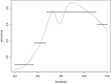
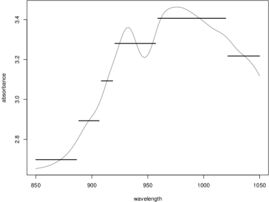
Figure 3: Piecewise constant approximations with 4 segments on the left and 6 segments on the right

2.4 Algorithmic cost

Given all the $Q\left(s,\{t_{k},\ldots,t_{l}\}\right)$, Algorithm 1 runs in $O(PM^{2})$. This is far more efficient that a naive approach in which all possible ordered partitions would be evaluated (there are $\frac{M!}{(M-P)!}$ such partitions). However, an efficient implementation is linked to a fast evaluation of the $Q\left(s,\{t_{k},\ldots,t_{l}\}\right)$. For instance, a naive implementation based on equation (6) leads to a $O(M^{3})$ cost that dominates the cost of Algorithm 1.

Fortunately, recursive formulation can be used to reduce in some cases the computation cost associated to the $Q\left(s,\{t_{k},\ldots,t_{l}\}\right)$ to $O(M^{2})$. As an illustration, Algorithm 2 computes $Q$ for equation (6) (piecewise constant approximation) in $O(M^{2})$.

Algorithm 2 Recursive calculation of $Q\left(s,\{t_{k},\ldots,t_{l}\}\right)$

1:  for $k=1$ to $M$ do

2:     $\mu(s,\{t_{k}\})\leftarrow s(t_{k})$

3:     $Q(s,\{t_{k}\})\leftarrow 0$

4:  end for

5:  for $l=2$ to $M$ do

6:     $\mu(s,\{t_{1},\ldots,t_{l}\})\leftarrow\frac{1}{l}\left[(l-1)\mu(s,\{t_{1},\ldots,t_{l-1}\})+s(t_{l})\right]$

7:     $Q(s,\{t_{1},\ldots,t_{l}\})\leftarrow Q(s,\{t_{1},\ldots,t_{l-1}\})+\frac{l}{l-1}\left[s(t_{l})-\mu(s,\{t_{1},\ldots,t_{l}\})\right]^{2}$

8:  end for

9:  for $k=2$ to $M-1$ do

10:     for $l=k+1$ to $M$ do

11:        $\mu(s,\{t_{k},\ldots,t_{l}\})\leftarrow\frac{1}{l-k+1}\left[(l-k+2)\mu(s,\{t_{k-1},\ldots,t_{l}\})-s(t_{k-1})\right]$

12:        $Q(s,\{t_{k},\ldots,t_{l}\})\leftarrow Q(s,\{t_{k-1},\ldots,t_{l}\})-\frac{l-k+1}{l-k+2}[s(t_{k-1})-\mu(s,\{t_{k},\ldots,t_{l}\})]^{2}$

13:     end for

14:  end for

Similar algorithms can be derived for other choices of the approximation solution used in each segment. The memory usage can also be reduced from $O(M^{2})$ in Algorithms 1 and 2 to $O(M)$ (see, e.g., [21, 22]).

2.5 Extensions and variations

As mentioned before, the general framework summarized in equation (9) is very flexible and accommodates numerous variations. Those variations include the approximation model (constant, linear, peak, etc.), the quality criterion (quadratic, absolute value, robust Huber loss [14], etc.) and the aggregation operator (sum or maximum of the point wise errors).

Figure 4 gives an application example: the spectrum from Figure 2 is approximated via a piecewise linear representation (on the right hand side of the Figure): as expected, the piecewise linear approximation is more accurate than the piecewise constant one, while the former uses less numerical parameters than the latter.

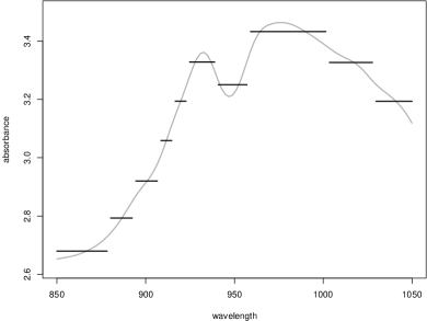
Figure 4: Segmentation of a single function: piecewise constant with 10 segments (left) versus piecewise linear with 5 segments (right)

Indeed, the piecewise linear approximation is easier to describe than the piecewise constant approximation: one needs only to specify the 4 breakpoints between the segments together with 10 extremal values, while the piecewise constant approximation needs 10 numerical values together with 9 breakpoints.

However, this example is particularly favorable for the piecewise linear approximation. Indeed, the independence hypothesis embedded in equation (9) and needed for the dynamic programming approach prevents us from introducing non local constraints in the approximating function. In particular, one cannot request for the piecewise linear approximation to be continuous. This is emphasized on Figure 4 by the disconnected drawing of the approximation function: in fact, the function $g$ is not defined between $t_{k}$ and $t_{k+1}$ if those two points belong to distinct clusters (in the case of Bellman’s solution [3], the function is not well defined at the boundaries of the intervals). Of course, one can use linear interpolation to connect $g(t_{k})$ with $g(t_{k+1})$, but this can introduce in practice $P-1$ additional very short segments, leading to an overly complex model.

In the example illustrated on Figure 4, the piecewise approximation does not suffer from large jumps between segments. Would that be the case, one could use an enriched description of the function specifying the starting and ending values on each segment. This would still be simpler than the piecewise constant description. However, if the original function is continuous, using a non continuous approximation can lead to false conclusion.

To illustrate the flexibility of the proposed framework beyond the simple variations listed above, we derive a solution to this continuity problem [22]. Let us first define

$$Q(s,\{t_{k},\ldots,t_{l}\})=\sum_{j=1}^{l}\left(s(t_{j})-\frac{(s(t_{k})-s(t_{l}))t+(t_{k}s(t_{l})-t_{l}s(t_{k}))}{t_{k}-t_{l}}\right)^{2}.$$ (12)

This corresponds to the total quadratic error made by the linear interpolation of $s$ on $\{t_{k},\ldots,t_{l}\}$ based on the two interpolation points $(t_{k},s(t_{k}))$ and $(t_{l},s(t_{l}))$. Then we replace the quality criterion of equation (9) by the following one:

$$E((k_{l})_{l=0}^{P})=\sum_{l=1}^{P}Q(s,\{t_{k_{l-1}},\ldots,t_{k_{l}}\}),$$ (13)

defined for an increasing series $(k_{l})_{l=0}^{P}$ with $k_{0}=1$ and $k_{P}=M$. Obviously, $E((k_{l})_{l=0}^{P})$ is the total quadratic error made by the piecewise linear interpolation of $s$ on $[t_{1},t_{M}]$ based on the $P+1$ interpolation points $(t_{k_{l}},s(t_{k_{l}}))_{l=0}^{P}$. While $(k_{l})_{l=0}^{P}$ does not correspond strictly to a partition of $\{t_{1},\ldots,t_{M}\}$ (because each interpolation point belongs to two segments, expect for the first and the last ones), the criterion $E$ is additive and has to be optimized on an ordered structure. As such, it can be minimized by a slightly modified version of Algorithm 1.

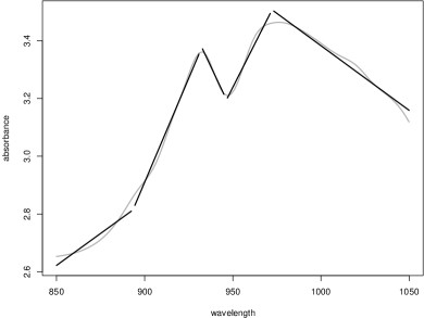
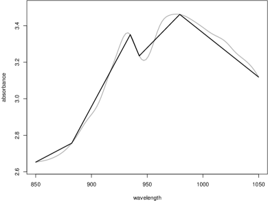
Figure 5: Segmentation of a single function: piecewise linear with 5 segments (left) versus linear interpolation with 5 segments (right)

Figure 5 shows the differences between the piecewise linear approach and the linear interpolation approach. For continuous functions, the latter seems to be more adequate than the former: it does not introduce arbitrary discontinuity in the approximating function and provides a simple summary of the original function.

The solutions explored in this section target specifically the summarizing issue by providing simple approximating function. As explained in Section 2.1, this rules out smooth approximation. In other applications context not addressed here, one can trade simplicity for smoothness. In [4], a model based approach is used to build a piecewise polynomial approximation of a function. The algorithm provides a segmentation useful for instance to identify underlying regime switching as well as a smooth approximation of the original noisy signal. While the method and framework are related, they oppose on the favored quality: one favors smoothness, the other favors simplicity.

3 Summarizing several functions

Let us now consider $N$ functions $(s_{i})_{i=1}^{N}$ sampled in $M$ distinct points $(t_{k})_{k=1}^{M}$ from the interval $[t_{1},t_{M}]$ (as in Section 2, the points are assumed to be ordered). Our goal is to leverage the function summarizing framework presented in Section 2 to build a summary of the whole set of functions. We first address the case of a homogeneous set of functions and tackle after the general case.

3.1 Single summary

Homogeneity is assumed with respect to the chosen functional metric, i.e., to the error criterion used for segmentation in Section 2, for instance the $L_{2}$ . Then a set of functions is homogeneous if its diameter is small compared to the typical variations of a function from the set. In the quadratic case, we request for instance to the maximal quadratic distance between two functions of the set to be small compared to the variances of functions of the set around their mean values.

Then, if the functions $(s_{i})_{i=1}^{N}$ are assumed to be homogeneous, finding a single summary function seems natural. In practice, this corresponds to finding a simple function $g$ that is close to each of the $s_{i}$ as measured by a functional norm: one should choose a summary type (e.g., piecewise constant), a norm (e.g., $L_{2}$) and a way to aggregate the individual comparison of each function to the summary (e.g., the sum of the norms).

Let us first consider the case of a piecewise constant function $g$ defined by $P$ intervals $(I_{p})_{p=1}^{P}$ (a partition of $[t_{1},t_{M}]$) and $P$ values $(a_{p})_{p=1}^{P}$ (with $g(t)=a_{p}$ when $t\in I_{p}$). If we measure the distance between $g$ and $s_{i}$ via the $L_{2}$ distances and consider the sum of $L_{2}$ distances as the target error measure, we obtain the following segmentation error:

$$E\left((s_{i})_{i=1}^{N},(I_{p})_{p=1}^{P},(a_{p})_{p=1}^{P}\right)=\sum_{i=1}^{N}\sum_{p=1}^{P}\sum_{t_{k}\in I_{p}}\left(s_{i}(t_{k})-a_{p}\right)^{2},$$ (14)

using the same quadrature scheme as in Section 2.2. Huygens’ theorem gives

$$\sum_{i=1}^{N}\left(s_{i}(t_{k})-a_{p}\right)^{2}=N\left(\mu(t_{k})-a_{p}\right)^{2}+\sum_{i=1}^{N}\left(s_{i}(t_{k})-\mu(t_{k})\right)^{2},$$ (15)

where $\mu=\frac{1}{N}\sum_{i=1}^{N}s_{i}$ is the mean function. Therefore minimizing $E$ from equation (14) is equivalent to minimizing

$$E^{\prime}\left((s_{i})_{i=1}^{N},(I_{p})_{p=1}^{P},(a_{p})_{p=1}^{P}\right)=\sum_{p=1}^{P}\sum_{t_{k}\in I_{p}}\left(\mu(t_{k})-a_{p}\right)^{2}.$$ (16)

In other words, the problem consists simply in building an optimal summary of the mean curve of the set and is solved readily with Algorithm 1. The additional computational cost induced by the calculation of the mean function is in $O(NM)$. This will generally be negligible compared to the $O(PM^{2})$ cost of the dynamic programming.

The reasoning above applies more generally to piecewise models used with the sum of $L_{2}$ distances. Indeed if $g(t)$ is such that $g(t)=g_{p}(t)$ when $t\in I_{p}$, then we have

$$\sum_{i=1}^{N}\left(s_{i}(t_{k})-g_{p}(t_{k})\right)^{2}=N\left(\mu(t_{k})-g_{p}(t_{k})\right)^{2}+\sum_{i=1}^{N}\left(s_{i}(t_{k})-\mu(t_{k})\right)^{2},$$ (17)

which leads to the same solution: $g$ can be obtained as the summary of the mean curve. The case of linear interpolation proposed in Section 2.5 is a bit different in the sense that interpolating several curves at the same time is not possible. Therefore, the natural way to extend the proposal to a set of curves it to interpolate the mean curve. An example of the result obtained by this method is given in Figure 6.

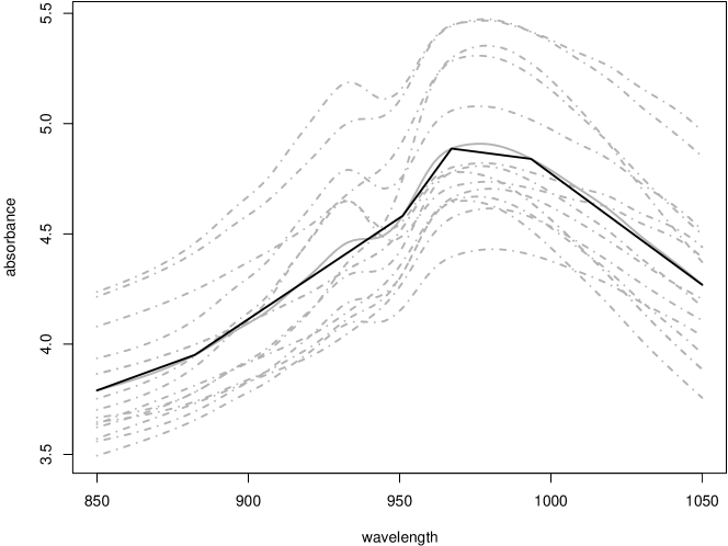
Figure 6: Group summary via an linear interpolation of the mean; the grey dashed/dotted curves are the original ones, the grey solid curve is the mean curve and the black curve is the piecewise linear interpolation curve that provides the group summary

In the general case, we assume given an error criterion $Q$ that applies to a set of contiguous evaluation points $\{t_{k},\ldots,t_{l}\}$: it gives the error done by the local model on $\{t_{k},\ldots,t_{l}\}$ as an approximation of all the functions $(s_{i})_{i=1}^{N}$. Then given an ordered partition of $\{t_{1},\ldots,t_{M}\}$, $(C_{p})_{p=1}^{P}$, we use the sum of the $Q((s_{i})_{i=1}^{N},C_{p})$ as a global error measure and obtain an additive form as in equation (9). Algorithm 1 applies straightforwardly (it applies also to taking, e.g., the maximum of the $Q((s_{i})_{i=1}^{N},C_{p})$ over $p$).

The only difficulty compared to the case of a unique function is the efficient calculation of the $Q((s_{i})_{i=1}^{N},\{t_{k},\ldots,t_{l}\})$. As shown above, the $L_{2}$ case is very favorable as it amounts to summarizing the mean curve. However, more complex norms and/or aggregation rules lead to difficulties. If we use for instance

$$Q((s_{i})_{i=1}^{N},\{t_{k},\ldots,t_{l}\})=\min_{a}\max_{1\leq i\leq N}\sum_{j=k}^{l}(s_{i}(t_{j})-a)^{2},$$ (18)

the problem cannot be formulated as a single curve summarizing problem, while is consists simply in considering the maximal $L_{2}$ distance rather than the sum of the $L_{2}$ distances: if the curves have different variances on $\{t_{k},\ldots,t_{l}\}$, the optimal value $a$ will not be the mean on the set of evaluation points of the mean curve. More generally, the computation of all $Q((s_{i})_{i=1}^{N},\{t_{k},\ldots,t_{l}\})$ might scale much faster than in $O(M(M+N))$ and thus might dominate the total computation time. Indeed, if there is no closed form expression for $Q$, then the value has to be computed from scratch for each pair $(k,l)$, which implies $O(M^{2})$ problem solving. Then, if no special structure or preprocessing can be used to simplify the problem, computing one value of $Q$ implies clearly to look at all the involved functions, i.e, to $O(N)$ observations. Therefore, if no simplification can be done, computing all values of $Q$ will imply at least at $O(NM^{2})$ calculation cost. Care must therefore be exercised when choosing the quality criterion and the summarizing model to avoid excessive costs. That said, the dynamic programming approach applies and leads to an optimal segmentation according to the chosen criterion.

3.2 Clustering

Assuming that a set of functions is homogeneous is too strong in practice, as shown on Figure 6: some of the curves have a small bump around 940 nm but the bump is very small in the mean curve. As a consequence, the summary misses this feature while the single curve summary used in Figure 5 was clearly picking up the bump.

It is therefore natural to rely on a clustering strategy to produce homogeneous clusters of curves and then to apply the method described in the previous section to summarize each cluster. However, the direct application of this strategy might lead to suboptimal solutions: at better solution should be obtained by optimizing at once the clusters and the associated summaries. We derive such an algorithm in the present section.

In a similar way to the previous section, we assume given an error measure $Q(G,\{t_{k},\ldots,t_{l}\})$ (where $G$ is a subset of $\{1,\ldots,N\}$): it measures the error made by the local model on the $\{t_{k},\ldots,t_{l}\}$ as an approximation of the functions $s_{i}$ for $i\in G$. For instance

$$Q(G,\{t_{k},\ldots,t_{l}\})=\min_{a}\sum_{i\in G}\sum_{j=k}^{l}(s_{i}(t_{j})-a)^{2},$$ (19)

for a constant local model evaluated with respect to the sum of $L_{2}$ distances. Let us assume for now that each cluster is summarized via a segmentation scheme that uses a cluster independent number of segments, $P/K$ (this value is assumed to be an integer). Then, given a partition of $\{1,\ldots,N\}$ into $K$ clusters $(G_{k})_{k=1}^{K}$ and given for each cluster an ordered partition of $\{t_{1},\ldots,t_{M}\}$, $(C^{k}_{p})_{p=1}^{P/K}$, the global error made by the summarizing scheme is

$$E\left((s_{i})_{i=1}^{N},(G_{k})_{k=1}^{K},\left((C^{k}_{p})_{p=1}^{P/K}\right)_{k=1}^{K}\right)=\sum_{k=1}^{K}\sum_{p=1}^{P/K}Q(G_{k},C^{k}_{p}).$$ (20)

Building an optimal summary of the set of curves amounts to minimizing this global error with respect to the function partition and, inside each cluster, with respect to the segmentation.

A natural way to tackle the problem is to apply an alternating minimization scheme (as used for instance in the K-means algorithm): we optimize successively the partition given the segmentation and the segmentation given the partition. Given the function partition $(G_{k})_{k=1}^{K}$, the error is a sum of independent terms: one can apply dynamic programming to build an optimal summary of each of the obtained clusters, as shown in the previous section. Optimizing with respect to the partition given the segmentation is a bit more complex as the feasibility of the solution depends on the actual choice of $Q$. In general however, $Q$ is built by aggregating via the maximum or the sum operators distances between the functions assigned to a cluster and the corresponding summary. It is therefore safe to assume that assigning a function to the cluster with the closest summary in term of the distance used to define $Q$ will give the optimal partition given the summaries. This leads to Algorithm 3.

Algorithm 3 Simultaneous clustering and segmentation algorithm (uniform case)

1:  initialize the partition $(G_{k})_{k=1}^{K}$ randomly

2:  repeat

3:     for $k=1$ to $K$ do

4:        apply Algorithm 1 to the find the optimal summary $g_{k}$ of the set of curves $\{s_{i}|i\in G_{k}\}$ in $P/K$ segments

5:     end for

6:     for $i=1$ to $N$ do

7:        assign $s_{i}$ to $G_{k}$ such that the distance between $s_{i}$ and $g_{k}$ is minimal over $k$

8:     end for

9:  until $(G_{k})_{k=1}^{K}$ is stable

The computational cost depends strongly on the availability of an efficient calculation scheme for $Q$. If this is the case, then the cost of the $K$ dynamic programming applications grows in $O(K(P/K)M^{2})=O(PM^{2})$. With standard $L_{p}$ distances between functions, the cost of the assignment phase is in $O(NKM)$. Computing the mean function in each cluster (or similar quantities such as the median function that might be needed to compute efficiently $Q$) has a negligible cost compared to the other costs (e.g., $O(NM)$ for the mean functions).

Convergence of Algorithm 3 is obvious as long as both the assignment phase (i.e., the minimization with respect to the partition given the segmentation) and the dynamic programming algorithm use deterministic tie breaking rules and lead to unique solutions. While the issue of ties between prototypes is generally not relevant in the K-means algorithm, for instance, it plays an important role in our context. Indeed, the summary of a cluster can be very simple and therefore, several summaries might have identical distance to a given curve. Then if ties are broken at random, the algorithm might never stabilize. Algorithm 1 is formulated to break ties deterministically by favoring short segments at the beginning of the segmentation (this is implied by the strict inequality test used at line 10 of the Algorithm). Then the optimal segmentation is unique given the partition, and the optimal partition is unique given the segmentation. As a consequence, the alternative minimization scheme converges.

Figure 7 gives an example of the results obtained by the algorithm in the case of a piecewise linear summary with five segments per cluster (the full Tecator dataset contains $N=240$ spectra with $M=100$ for each spectrum).

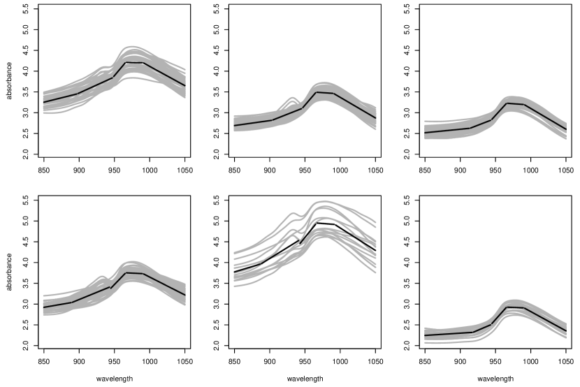
Figure 7: Summary of the full Tecator dataset with 6 clusters and 5 segments per cluster: grey curves are the original spectra, dark curves are the summaries for each cluster

In practice, we will frequently use a piecewise constant model whose quality is assessed via the sum of the $L_{2}$ distances, as in equation (19). Then equation (20) can be instantiated as follows:

$$E\left((s_{i})_{i=1}^{N},(G_{k})_{k=1}^{K},\left((C^{k}_{p})_{p=1}^{P/K}\right)_{k=1}^{K}\right)=\sum_{k=1}^{K}\sum_{i\in G_{k}}\sum_{p=1}^{P/K}\sum_{t_{j}\in C^{k}_{p}}\left(s_{i}(t_{j})-\mu_{k,p}\right)^{2},$$ (21)

with

$$\mu_{k,p}=\frac{1}{|G_{k}||C^{k}_{p}|}\sum_{i\in G_{k}}\sum_{t_{j}\in C^{k}_{p}}s_{i}(t_{j}).$$ (22)

Let us denote $\mathbf{s}_{i}=(s_{i}(t_{1}),\ldots,s_{i}(t_{M}))$ the $\mathbb{R}^{M}$ vector representation of the sampled functions and $\mathbf{g}_{k}=(g_{k}(t_{1}),\ldots,g_{k}(t_{M}))$ the vector representation of the piecewise constant functions defined by $g_{k}(t_{i})=\mu_{k,p}$ when $t_{i}\in C^{k}_{p}$. Then equation (21) can be rewritten

$$E\left((\mathbf{s}_{i})_{i=1}^{N},(G_{k})_{k=1}^{K},\left((C^{k}_{p})_{p=1}^{P}\right)_{k=1}^{K}\right)=\sum_{k=1}^{K}\sum_{i\in G_{k}}\|\mathbf{s}_{i}-\mathbf{g}_{k}\|^{2}.$$ (23)

This formulation emphasizes the link between the proposed approach and the K means algorithm. Indeed the criterion is the one optimized by the K means algorithm for the vector data $\mathbf{s}_{i}$ with a constraint on the prototypes: rather than allowing arbitrary prototypes as in the standard K means, we use simple prototypes in the sense of Section 2.1. Any piecewise model whose quality is assessed via the sum of the $L_{2}$ distances leads to the same formulation, but with different constraints on the shape of the functional prototypes.

Equation (23) opens the way to many variations on the same theme: most of the prototype based clustering methods can be modified to embed constraints on the prototypes, as Algorithm 3 does for the K means. Interesting candidates for such a generalization includes the Self Organizing Map in its batch version [18], Neural Gas also in its batch version [7] and deterministic annealing based clustering [27], among others.

3.3 Optimal resources allocation

A drawback of Algorithm 3 is that it does not allocate resources in an optimal way: we assumed that each summary will use $P/K$ segments, regardless of the cluster. Fortunately, dynamic programming can be used again to remove this constraint. Let us consider indeed a resource assignment, that is $K$ positive integers $(P_{k})_{k=1}^{K}$ such that $\sum_{k=1}^{K}P_{k}=P$. The error made by the summarizing scheme when cluster $G_{k}$ uses $P_{k}$ segments for its summary is given by

$$E\left((s_{i})_{i=1}^{N},(G_{k})_{k=1}^{K},(P_{k})_{k=1}^{K},\left((C^{k}_{p})_{p=1}^{P_{k}}\right)_{k=1}^{K}\right)=\sum_{k=1}^{K}\sum_{p=1}^{P_{k}}Q(G_{k},C^{k}_{p}).$$ (24)

As for the criterion given by equation (20) in the previous section, we rely on an alternating minimization scheme. Given the function partition $(G_{k})_{k=1}^{K}$, the challenge is to optimize $E$ with respect to both the resource assignment and the segmentation. For a fixed partition $(G_{k})_{k=1}^{K}$, let us denote

$$R_{k}(P_{k})=\min_{(C^{k}_{p})_{p=1}^{P_{k}}\text{ ordered partition of }\{t_{1},\ldots,t_{M}\}}\sum_{p=1}^{P_{k}}Q(G_{k},C^{k}_{p})$$ (25)

Then minimizing $E$ from equation (24) for a fixed partition $(G_{k})_{k=1}^{K}$ corresponds to minimizing:

$$U\left((P_{k})_{k=1}^{K}\right)=\sum_{k=1}^{K}R_{k}(P_{k})$$ (26)

with respect to the resource assignment. This formulation emphasizes two major points.

Firstly, as already mentioned in Section 2.3, given a number of segments $P$ Algorithm 1 and its variants provide with a negligible additional cost all the optimal segmentations in $p=1$ to $P$ segments. Therefore, the calculation of $R_{k}(p)$ for $p\in\{1,\ldots,P\}$ can be done with a variant of Algorithm 1 in $O(PM^{2})$ provided an efficient calculation of $Q(G_{k},C^{k}_{p})$ is possible (in fact, one needs only values of $R_{k}(p)$ for $p\leq P-K+1$ as we request at least one segment per cluster, but to ease the calculation we assume that we compute values up to $P$).

Secondly, $U$ as defined in equation (26) is an additive measure and can therefore be optimized by dynamic programming. Indeed let us define $S(l,p)$ as

$$S(l,p)=\min_{(P_{k})_{k=1}^{l}\text{ such that }\sum_{k=1}^{l}P_{k}=p}\sum_{k=1}^{l}R_{k}(P_{k})$$ (27)

The $S(1,p)$ are readily obtained from the optimal segmentation algorithm ($S(1,p)=R_{1}(p)$). Then the additive structure of equation (26) shows that

$$S(l,p)=\min_{1\leq u\leq p-l+1}S(l-1,p-u)+R_{l}(u).$$ (28)

Given all the $R_{l}(p)$ the calculation of $S(K,P)$ has therefore a cost of $O(KP^{2})$. This calculation is plugged into Algorithm 3 to obtain Algorithm 4.

Algorithm 4 Simultaneous clustering and segmentation algorithm with optimal resource assignment

1:  initialize the partition $(G_{k})_{k=1}^{K}$ randomly

2:  repeat

3:     for $k=1$ to $K$ do

4:        apply Algorithm 1 to compute $R_{k}(p)$ for all $p\in\{1,\ldots,P-K+1\}$

5:     end for

6:     for $p=1$ to $P-K+1$ do {initialisation of the resource allocation phase}

7:        $S(1,p)\leftarrow R_{1}(p)$

8:     end for

9:     for $l=2$ to $K$ do {dynamic programming for resource allocation}

10:        for $p=l$ to $P$ do

11:           $W(l,p)\leftarrow 1$

12:           $S(l,p)\leftarrow S(l-1,p-1)+R_{l}(1)$

13:           for $u=2$ to $p-l+1$ do

14:              if $S(l-1,p-u)+R_{l}(u)<S(l,p)$ then

15:                 $W(l,p)\leftarrow u$

16:                 $S(l,p)\leftarrow S(l-1,p-u)+R_{l}(u)$

17:              end if

18:           end for

19:        end for

20:     end for

21:     $P_{opt}\leftarrow(\text{NA},\ldots,\text{NA})$ {backtracking phase}

22:     $P_{opt}(K)\leftarrow W(K,P)$

23:     $availabe\leftarrow P-W(K,P)$

24:     for $k=K-1$ to $1$ do

25:        $P_{opt}(k)\leftarrow W(k,available)$

26:        $availabe\leftarrow availabe-W(k,available)$

27:     end for

28:     for $k=1$ to $K$ do {summary calculation}

29:        build $g_{k}$ with $P_{opt}(k)$ segments

30:     end for

31:     for $i=1$ to $N$ do

32:        assign $s_{i}$ to $G_{k}$ such that the distance between $s_{i}$ and $g_{k}$ is minimal over $k$

33:     end for

34:  until $(G_{k})_{k=1}^{K}$ is stable

Given the values of $Q$, the total computational cost of the optimal resource assignment and of the optimal segmentation is therefore in $O(KP(M^{2}+P))$. As we target simple descriptions, it seems reasonable to assume that $P\ll M^{2}$ and therefore that the cost is dominated by $O(KPM^{2})$. Then, using the optimal resource assignment multiplies by $K$ the computational cost compared to a uniform use of $P/K$ segments per cluster (which computational cost is in $O(PM^{2})$). The main source of additional computation is the fact that one has to study summaries using $P$ segments for each cluster rather than only $P/K$ in the uniform case. This cost can be reduced by introducing an arbitrary (user chosen) maximal number of segments in each clusters, e.g., $\lambda P/K$. Then the running time of the optimal assignment is $\lambda$ times the running time of the uniform solution. As we aim at summarizing the data, using a small $\lambda$ such $2$ seems reasonable.

The computation of the values of $Q$ remains the same regardless of the way the number of segments is chosen for each cluster. The optimisation of the error with respect to the partition $(G_{k})_{k=1}^{K}$ follows also the same algorithm in both cases. If we use for instance piecewise constant approximation evaluated with the sum of the $L_{2}$ distances, then, as already mentioned previously, the summaries are computed from the cluster means: computing the means costs $O(NM)$, then the calculation of $Q$ for all functional clusters is in $O(KM^{2})$ and the optimization with respect to $(G_{k})_{k=1}^{K}$ is in $O(NKM)$. In general, the dominating cost will therefore scale in $O(KPM^{2})$. However, as pointed out in Section 3.1, complex choices for the $Q$ error criterion may induce larger computational costs.

3.4 Two phases approaches

The main motivation of the introduction of Algorithm 3 was to avoid relying on a simpler but possibly suboptimal dual phases solution. This alternative solution simply consists applying a standard K means to the vector representation of the functions $(s_{i})_{i=1}^{N}$ to get homogeneous clusters and then to summarize each cluster via a simple prototype. While this approach should intuitively give higher errors for the criterion of equation (20), the actual situation is more complex.

Algorithms 3 and 4 are both optimal in their segmentation phase and will generally be also optimal for the partition determination phase if $Q$ is a standard criterion. However, the alternating optimization scheme itself is not optimal (the K means algorithm is also non optimal for the same reason). We have therefore no guarantee on the quality of the local optimum reached by those algorithms, exactly as in the case of the K means. In addition, even if the two phase approach is initialized with the same random partition as, e.g., Algorithm 3, the final partitions can be distinct because of the distinct prototypes used during the iterations. It is therefore difficult to predict which approach is more likely to give the best solution. In addition a third possibility should be considered: the K means algorithm is applied to the vector representation of the functions $(s_{i})_{i=1}^{N}$ to get homogeneous clusters and is followed by an application of Algorithm 3 or 4 using the obtained clusters for its initial configuration.

To assess the differences between these three possibilities, we conducted a simple experiment: using the full Tecator dataset, we compared the value of $E$ from equation (20) for the final summary obtained by the three solutions using the same random starting partitions with $K=6$, $P=30$ and piecewise constant summaries. We used 50 random initial configurations and compared the methods in the case of uniform resource allocation ($5$ segments per cluster) and in the case of optimal resource allocation.

In the case of uniform resources assignment the picture is rather simple. For all the 50 random initialisations both two phases algorithms gave exactly the same results. In 44 cases, using Algorithm 3 gave exactly the same results as the two phases algorithms. In 5 cases, its results were of lower quality and in the last case, its results were slightly better. The three algorithms manage to reach the same overall optimum (for which $E=472$).

The case of optimal resources assignment is a bit more complex. For 15 out of 50 initial configurations, using Algorithm 4 after the K means improves the results over a simple optimal summary (with optimal resource assignment) applied to the results of the K means (results were identical for the 35 other cases). In 34 cases, K means followed by Algorithm 4 gave the same results as Algorithm 4 alone. In the 16 remaining cases, results are in favor of K means followed by Algorithm 4 which wins 13 times. Nevertheless, the three algorithms manage to reach the same overall optimum (for which $E=467$).

While there is no clear winner in this (limited scope) experimental analysis, considering the computational cost of the three algorithms helps choosing the most appropriate one in practice. In favorable cases, the cost of an iteration of Algorithm 4 is $O(KMN+KPM^{2}))$ while the cost of an iteration of the K means on the same dataset is $O(KMN)$. In functional data, $M$ is frequently of the same order as $N$. For summarizing purposes, $P$ should remain small, around $5K$ for instance. This means that one can perform several iterations of the standard K means for the same computational price than one iteration of Algorithm 4. For instance, the Tecator dataset values, $P=30$, $M=100$ and $N=240$, give $1+PM/N=13.5$. In the experiments described above, the median number of iterations for the K means was 15 while it was respectively 15 and 16 for Algorithms 3 and 4. We can safely assume therefore that Algorithm 4 is at least 10 times slower than the K means on the Tecator dataset. However, when initialized with the K means solution, Algorithms 3 and 4 converges very quickly, generally in two iterations (up to five for the optimal assignment algorithm in the Tecator dataset). In more complex situations, as the ones studied in Section 4 the number of iterations is larger but remains small compared to what would be needed when starting from a random configuration.

Based on the previous analysis, we consider that using the K means algorithm followed by Algorithm 4 is the best solution. If enough computing resources are available, one can run the K means algorithm from several starting configurations, keep the best final partition and use it as an initialization point for Algorithm 4. As the K means provides a good starting point to this latter algorithm, the number of iterations remains small and the overall complexity is acceptable, especially compared to using Algorithm 4 alone from different random initial configurations. Alternatively, the analyst can rely on more robust clustering scheme such as Neural Gas [7] and deterministic annealing based clustering [27], or on the Self Organizing Map [18] to provide the starting configuration of Algorithm 4.

4 Experimental results

We give in this section two examples of the type of exploratory analyses that can be performed on real world datasets with the proposed method. In order to provide the most readable display for the user, we build the initial configuration of Algorithm 4 with a batch Self Organizing Map. We optimize the initial radius of the neighborhood influence in the SOM with the help of the Kaski and Lagus topology preservation criterion [17] (the radius is chosen among 20 radii).

4.1 Topex/Poseidon satellite

We study first the Topex/Poseidon satellite dataset. The Topex/Poseidon radar satellite has been used over the Amazonian basin to produce $N=472$ waveforms sampled at $M=70$ points. The curves exhibit a quite large variability induced by differences in ground type below the satellite during data acquisition. Details on the dataset can be found in e.g. [11, 12]. Figure 8 displays 20 curves from the dataset chosen randomly.

Figure 8: 20 curves from the Topex/Poseidon radar satellite dataset

Figure 9: Dendrogram of the hierarchical clustering for the Topex/Poseidon radar satellite dataset

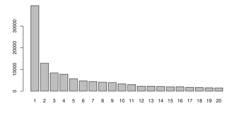
Figure 10: Total within class variance decrease for the 20 first merges in the dendrogram depicted by Figure 9

We conduct first a hierarchical clustering (based on Euclidean distance between the functions and the Ward criterion) to get a rough idea of the potential number of clusters in the dataset. Both the dendrogram (Figure 9) and the total within class variance evolution (Figure 10) tend to indicate a rather small number of clusters, around 12. As the visual representation obtained via the SOM is more readable than a randomly arranged set of prototypes, we can use a slightly oversized SOM without impairing the analyst’s work. We decided therefore to use a $4\times 5$ grid: the rectangular shape has been preferred over a square one according to results from [34] that show some superiority in topology preservation for anisotropic maps compared to isotropic ones.

Figure 11: Prototypes obtained by SOM algorithm on the Topex/Poseidon radar satellite dataset (grey curves are the original curves as assigned to the clusters)

The results of the SOM are given in Figure 11 that displays the prototype of each cluster arranged on the SOM grid. Each cell contains also all the curves assigned to the associated clusters. As expected, the SOM prototypes are well organized on the grid: the horizontal axis seems to encode approximately the position of the maximum of the prototype while the vertical axis corresponds to the width of the peak. However, the prototypes are very noisy and inferring the general behavior of the curves of a cluster remains difficult.

Figure 12: Summarized prototypes obtained by Algorithm 4 on the Topex/Poseidon radar satellite dataset (grey curves are the original curves as assigned to the clusters)

Figure 12 represents the results obtained after applying Algorithm 4 to the results of the SOM. In order to obtain a readable summary, we set $P$ to $80$, i.e., an average of 4 segments for each cluster. We use the linear interpolation approach described in Section 2.5. Contrarily to results obtained on the Tecator dataset and reported in Section 3.4, Algorithm 4 used a significant number of iterations (17). Once the new clusters and the simplified prototypes were obtained, they were displayed in the same way as for the SOM results. The resulting map is almost as well organized as the original one (with the exception of a large peak on the bottom line), but the simplified prototypes are much more informative than the original ones: they give an immediate idea of the general behavior of the curves in the corresponding cluster. For example, the differences between the two central prototypes of the second line (starting from the top) are more obvious with summaries: in the cluster on the left, one can identify a slow increase followed by a two phases slow decrease, while the other cluster corresponds to a sharp increase followed by a slow decrease. Those differences are not as obvious on the original map.

4.2 Electric power consumption

The second dataset consists in the electric power consumption recorded in a personal home during almost one year (349 days). Each curve consists in 144 measures which give the power consumption of one day at a 10 minutes sampling rate. Figure 13 displays 20 randomly chosen curves.

Figure 13: 20 electric power consumption curves

We analyse the curves in a very similar way as for the Topex/Poseidon dataset The results of the hierarchical clustering displayed by Figures 14 and 15 lead to the same conclusion as in the previous case: the number of clusters seems to be small, around 13. As before, we fit a slightly larger SOM ($4\times 5$ rectangular grid) to the data and obtain the representation provided by Figure 16. The map is well organized: the vertical axis seems to encode the global power consumption while the horizontal axis represents the overall shape of the load curve. However, the shapes of the prototypes are again not easy to interpret, mainly because of their noisy nature.

Figure 14: Dendrogram of the hierarchical clustering for the load curves

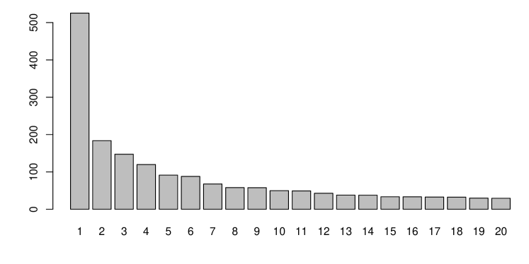
Figure 15: Total within class variance decrease for the 20 first merges in the dendrogram depicted by Figure 14

Figure 16: Prototypes obtained by SOM algorithm for the load curves (grey curves are the original curves as assigned to the clusters)

Figure 17 shows the results obtained after applying Algorithm 4 to the results of the SOM (Algorithm 4 used 9 iterations to reach a stable state). In order to obtain a readable summary, we set $P$ to $80$, i.e., an average of 4 segments for each cluster. We depart from the previous analysis by using here a piecewise constant summary: this is more adapted to load curves as they should be fairly constant on significant time periods, because many electrical appliances have stable power consumption once switched on. As for the Topex/Poseidon dataset, the summarized prototypes are much easier to analyze than their noisy counterpart. Even the global organization of the map is more obvious: the top right of the map for instance, gathers days in which the power consumption in the morning (starting at 7 am) is significant, is followed by a period of low consumption and then again by a consumption peak starting approximately at 7 pm. Those days are week days in which the home remains empty during work hours. Other typical clusters include holidays with almost no consumption (second cluster on the first line), more constant days which correspond to week ends, etc. In addition, the optimal resource assignment tends to emphasize the difference between the clusters by allocating less resources to simple ones (as expected). This is quite obvious in the case of piecewise constant summaries used in Figure 17 (and to a lesser extent on Figure 12).

Figure 17: Summarized prototypes ($P=80$) obtained by Algorithm 4 for the load curves (grey curves are the original curves as assigned to the clusters)

In order to emphasize the importance of a drastic reduction in prototype complexity, Algorithm 4 was applied to the same dataset, using the same initial configuration, with $P=160$, i.e., an average of 8 segments in each cluster. Results are represented on Figure 18.

Figure 18: Summarized prototypes ($P=160$) obtained by Algorithm 4 for the load curves (grey curves are the original curves as assigned to the clusters)

As expected, prototypes are more complex than on Figure 17. While they are not as rough as the original ones (see Figure 16), their analysis is more difficult than the one of prototypes obtained with stronger summarizing constraints. In particular, some consumption peaks are no more roughly outlined as in Figure 17 but more accurately approximated (see for instance the last cluster of the second row). This leads to series of short segments from which expert inference is not easy. It should be noted in addition, that because of the noisy nature of the data, increasing the number of segments improves only marginally the approximation quality. To show this, we first introduce a relative approximation error measure given by

$$\frac{\sum_{k=1}^{K}\sum_{i\in G_{k}}\sum_{p=1}^{P_{k}}\sum_{t_{j}\in C^{k}_{p}}(s_{i}(t_{j})-\mu_{k,p})^{2}}{\sum_{i=1}^{N}\sum_{j=1}^{M}(s_{i}(t_{j})-\mu_{i})^{2}},$$ (29)

using notations from Section 3.2, and where $\mu_{i}$ denotes the mean of $s_{i}$. This relative error compares the total squared approximation error to the total squared internal variability inside the dataset. Table 1 gives the dependencies between the number of segments and the relative approximation error. It is quite clear that the relative loss in approximation precision is acceptable even with strong summarizing constraints.

Summary	No summary	$P=160$	$P=80$
Relative approximation error	0.676	0.696	0.740

Table 1: Approximation errors for the load curves

This type of numerical quality assessment should be provided to the analyst either as a way to control the relevance of the summarized prototypes, or as a selection guide for choosing the value of $P$.

5 Conclusion

We have proposed in this paper a new exploratory analysis method for functional data. This method relies on simple approximations of functions, that is on models that are piecewise constant or piecewise linear. Given a set of homogeneous functions, a dynamic programming approach computes efficiently and optimally a simple model via a segmentation of the interval on which the functions are evaluated. Given several groups of homogeneous functions and a total number of segments, another dynamic programming algorithm allocates optimally to each cluster the number of segments used to build the summary. Finally, those two algorithms can be embedded in any classical prototype based algorithm (such as the K means) to refine the groups of functions given the optimal summaries and vice versa in an alternating optimization scheme.

The general framework is extremely flexible and accommodates different types of quality measures ($L_{2}$, $L_{1}$), aggregation strategies (maximal error, mean error), approximation model (piecewise constant, linear interpolation) and clustering strategies (K means, Neural gas). Experiments show that it provides meaningful summaries that help greatly the analyst in getting quickly a good idea of the general behavior of a set of curves.

While we have listed many variants of the method to illustrate its flexibility, numerous were not mentioned as they are more distant from the main topic of this paper. It should be noted for instance that rather than building a unique summary for a set of curves, one could look for a unique segmentation supporting curve by curve summaries. In other words, each curve will be summarized by e.g., a piecewise constant model, but all models will share the same segmentation. This strategy is very interesting for analyzing curves in which internal changes are more important than the actual values taken by the curves. It is closely related to the so called best basis problem in which a functional basis is built to represent efficiently a set of curves (see e.g., [5, 31, 28]). This is also related to variable clustering methods (see e.g., [19]). This final link opens an interesting perspective for the proposed method. It has been shown recently [10, 20] that variable clustering methods can be adapted to supervised learning: variables are grouped in a way that preserves as much as possible the explanatory power of the reduced set of variables with respect to a target variable. It would be extremely useful to provide the analyst with such a tool for exploring a set of curves: she would be able to select an explanatory variable and to obtain summaries of those curves that mask details that are not relevant for predicting the chosen variable.

References

- Abraham et al. [2003] C. Abraham, P.-A. Cornillon, E. Matzner-Lober, and N. Molinari. Unsupervised curve clustering using b-splines. Scandinavian Journal of Statistics, 30(3):581–595, September 2003.
- Auger and Lawrence [1989] I. E. Auger and C. E. Lawrence. Algorithms for the optimal identification of segment neighborhoods. Bulletin of Mathematical Biology, 51(1):39–54, 1989.
- Bellman [1961] R. Bellman. On the approximation of curves by line segments using dynamic programming. Communication of the ACM, 4(6):284, 1961.
- Chamroukhi et al. [2009] F. Chamroukhi, A. Samé, G. Govaert, and P. Aknin. A regression model with a hidden logistic process for signal parametrization. In Proceedings of XVIth European Symposium on Artificial Neural Networks (ESANN 2009), pages 503–508, Bruges, Belgique, April 2009.
- Coifman and Wickerhauser [1992] R. R. Coifman and M. V. Wickerhauser. Entropy-based algorithms for best basis selection. IEEE Transactions on Information Theory, 38(2):713–718, March 1992.
- Cottrell et al. [1998] M. Cottrell, B. Girard, and P. Rousset. Forecasting of curves using a kohonen classification. Journal of Forecasting, 17:429–439, 1998.
- Cottrell et al. [2006] M. Cottrell, B. Hammer, A. Hasenfuß, and T. Villmann. Batch and median neural gas. Neural Networks, 19(6–7):762–771, July–August 2006.
- Debrégeas and Hébrail [1998] A. Debrégeas and G. Hébrail. Interactive interpretation of kohonen maps applied to curves. In Proc. International Conference on Knowledge Discovery and Data Mining (KDD’98), pages 179–183, New York, August 1998.
- Devroye et al. [1996] L. Devroye, L. Györfi, and G. Lugosi. A Probabilistic Theory of Pattern Recognition, volume 21 of Applications of Mathematics. Springer, 1996.
- François et al. [2008] D. François, C. Krier, F. Rossi, and M. Verleysen. Estimation de redondance pour le clustering de variables spectrales. In Actes des 10èmes journées Européennes Agro-industrie et Méthodes statistiques (Agrostat 2008), pages 55–61, Louvain-la-Neuve, Belgique, January 2008.
- Frappart [2003] F. Frappart. Catalogue des formes d’onde de l’altimètre topex/poséidon sur le bassin amazonien. Rapport technique, CNES, Toulouse, France, 2003.
- Frappart et al. [2006] F. Frappart, S. Calmant, M. Cauhopé, F. Seyler, and A. Cazenave. Preliminary results of envisat ra-2-derived water levels validation over the amazon basin. Remote Sensing of Environment, 100(2):252 – 264, 2006. ISSN 0034-4257.
- Healey et al. [1995] C. G. Healey, K. S. Booth, and J. T. Enns. Visualizing real-time multivariate data using preattentive processing. ACM Transactions on Modeling and Computer Simulation, 5(3):190–221, July 1995.
- Huber [1964] P. J. Huber. Robust estimation of a location parameter. Annals of Mathematical Statistics, 35(1):73–101, 1964.
- Hugueney [2006] B. Hugueney. Adaptive segmentation-based symbolic representations of time series for better modeling and lower bounding distance measures. In Proceedings of 10th European Conference on Principles and Practice of Knowledge Discovery in Databases, PKDD 2006, volume 4213 of Lecture Notes in Computer Science, pages 545–552, September 2006.
- Jackson et al. [2005] B. Jackson, J. Scargle, D. Barnes, S. Arabhi, A. Alt, P. Gioumousis, E. Gwin, P. Sangtrakulcharoen, L. Tan, and T. T. Tsai. An algorithm for optimal partitioning of data on an interval. IEEE Signal Processing Letters, 12(2):105–108, Feb. 2005.
- Kaski and Lagus [1996] S. Kaski and K. Lagus. Comparing self-organizing maps. In C. von der Malsburg, W. von Seelen, J. Vorbrüggen, and B. Sendhoff, editors, Proceedings of International Conference on Artificial Neural Networks (ICANN’96), volume 1112 of Lecture Notes in Computer Science, pages 809–814. Springer, Berlin, Germany,, July 16-19 1996.
- Kohonen [1995] T. Kohonen. Self-Organizing Maps, volume 30 of Springer Series in Information Sciences. Springer, third edition, 1995. Last edition published in 2001.
- Krier et al. [2008] C. Krier, F. Rossi, D. François, and M. Verleysen. A data-driven functional projection approach for the selection of feature ranges in spectra with ica or cluster analysis. Chemometrics and Intelligent Laboratory Systems, 91(1):43–53, March 2008.
- Krier et al. [2009] C. Krier, M. Verleysen, F. Rossi, and D. François. Supervised variable clustering for classification of nir spectra. In Proceedings of XVIth European Symposium on Artificial Neural Networks (ESANN 2009), pages 263–268, Bruges, Belgique, April 2009.
- Lechevallier [1976] Y. Lechevallier. Classification automatique optimale sous contrainte d’ordre total. Rapport de recherche 200, IRIA, 1976.
- Lechevallier [1990] Y. Lechevallier. Recherche d’une partition optimale sous contrainte d’ordre total. Rapport de recherche RR-1247, INRIA, June 1990. http://www.inria.fr/rrrt/rr-1247.html.
- Lee and Verleysen [2005] J. A. Lee and M. Verleysen. Generalization of the lp norm for time series and its application to self-organizing maps. In Proceedings of the 5th Workshop on Self-Organizing Maps (WSOM 05), pages 733–740, Paris (France), September 2005.
- Lin et al. [2003] J. Lin, E. J. Keogh, S. Lonardi, and B. Y. chi Chiu. A symbolic representation of time series, with implications for streaming algorithms. In M. J. Zaki and C. C. Aggarwal, editors, DMKD, pages 2–11. ACM, 2003.
- Picard et al. [2007] F. Picard, S. Robin, E. Lebarbier, and J.-J. Daudin. A segmentation/clustering model for the analysis of array cgh data. Biometrics, 63(3):758–766, 2007.
- Ramsay and Silverman [1997] J. Ramsay and B. Silverman. Functional Data Analysis. Springer Series in Statistics. Springer Verlag, June 1997.
- Rose [1998] K. Rose. Deterministic annealing for clustering, compression,classification, regression, and related optimization problems. Proceedings of the IEEE, 86(11):2210–2239, November 1998.
- Rossi and Lechevallier [2008] F. Rossi and Y. Lechevallier. Constrained variable clustering for functional data representation. In Proceedings of the first joint meeting of the Société Francophone de Classification and the Classification and Data Analysis Group of the Italian Statistical Society (SFC-CLADAG 2008), Caserta, Italy, June 2008.
- Rossi et al. [2004] F. Rossi, B. Conan-Guez, and A. El Golli. Clustering functional data with the SOM algorithm. In Proceedings of XIIth European Symposium on Artificial Neural Networks (ESANN 2004), pages 305–312, Bruges (Belgium), April 2004.
- Rossi et al. [2007] F. Rossi, D. François, V. Wertz, and M. Verleysen. Fast selection of spectral variables with b-spline compression. Chemometrics and Intelligent Laboratory Systems, 86(2):208–218, April 2007.
- Saito and Coifman [1995] N. Saito and R. R. Coifman. Local discriminant bases and their applications. Journal of Mathematical Imaging and Vision, 5(4):337–358, 1995.
- Stone [1961] H. Stone. Approximation of curves by line segments. Mathematics of Computation, 15(73):40–47, 1961.
- Tikhonov and Arsenin [1979] A. N. Tikhonov and V. Y. Arsenin. Solutions of ill-posed problems. SIAM Review, 21(2):266–267, April 1979.
- Ultsch and Herrmann [2005] A. Ultsch and L. Herrmann. The architecture of emergent self-organizing maps to reduce projection errors. In Proceedings of the 13th European Symposium on Artificial Neural Networks (ESANN 2005), pages 1–6, Bruges (Belgium), April 2005.