Rectifiable ${\cal PT}-$symmetric Quantum Toboggans with Two Branch Points

Miloslav Znojil

Nuclear Physics Institute ASCR, 250 68 Řež, Czech Republic

Abstract

Certain complex-contour (a.k.a. quantum-toboggan) generalizations of Schrödinger’s bound-state problem are reviewed and studied in detail. Our key message is that the practical numerical solution of these atypical eigenvalue problems may perceivably be facilitated via an appropriate complex change of variables which maps their multi-sheeted complex domain of definition to a suitable single-sheeted complex plane.

PACS 03.65.Ge

1 Introduction

One-dimensional Schrödinger equation for bound states

$$-\frac{\hbar^{2}}{2m}\,\frac{d^{2}}{dx^{2}}\,\psi_{n}(x)+V(x)\,\psi_{n}(x)=E_{n}\,\psi_{n}(x)\,,\ \ \ \ \ \ \ \ \psi_{n}(x)\in\mathbb{L}^{2}(\mathbb{R})$$ (1)

belongs among the most friendly phenomenological models in quantum mechanics [1]. For virtually all of the reasonable phenomenological confining potentials $V(x)$ the numerical treatment of this eigenvalue problem remains entirely routine.

During certain recent numerical experiments [2] it became clear that many standard (e.g., Runge-Kutta [3]) computational methods may still encounter new challenges when one follows the advice by Bender and Turbiner [4], by Buslaev and Grecchi [5], by Bender et al [6] or by Znojil [7] and when one replaces the most common real line of coordinates $x\in\mathbb{R}$ in ordinary differential Eq. (1) by some less trivial complex contour of $x\in{\cal C}(s)$ which may be conveniently parametrized, whenever necessary, by a suitable real pseudocoordinate $s\in\mathbb{R}$,

$$-\frac{\hbar^{2}}{2m}\,\frac{d^{2}}{dx^{2}}\,\psi_{n}(x)+V(x)\,\psi_{n}(x)=E_{n}\,\psi_{n}(x)\,,\ \ \ \ \ \ \ \ \psi_{n}(x)\in\mathbb{L}^{2}({\cal C})\,.$$ (2)

Temporarily, the scepticism has been suppressed by Weideman [8] who showed that many standard numerical algorithms may be reconfirmed to lead to reliable results even for many specific analytic samples of complex interactions $V(x)$ giving real spectra via Eq. (2).

Unfortunately, the scepticism reemerged when we proposed, in Ref. [7], to study the so called quantum toboggans characterized by the relaxation of the most common tacit assumption that the above-mentioned integration contours ${\cal C}(s)$ must always lie just inside a single complex plane ${\cal R}_{0}$ equipped by suitable cuts. Subsequently, the reemergence of certain numerical difficulties accompanying the evaluation of the spectra of quantum toboggans has been reported by Bíla [9] and by Wessels [10]. Their empirical detection of the presence of instabilities in their numerical results may be recognized as one of the key motivations of our present considerations.

2 Illustrative tobogganic Schrödinger equations

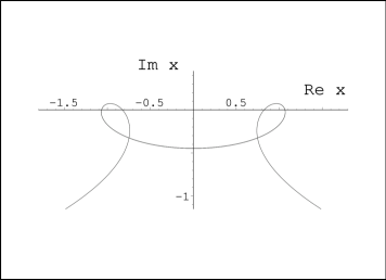
Figure 1: The central segment of the typical ${\cal PT}-$symmetric double-circle tobogganic curve of $x\in{\cal C}^{(LR)}(s)$ with winding parameter $\kappa=3$ in Eq. (10). This curve is obtained as the image of the straight line of $z\in{\cal C}^{(0)}(s)$ at $\varepsilon=0.250$.

2.1 Assumptions

Figure 2: An alternative version of the double-circle curve of Figure 1 obtained at the “almost maximal” $\varepsilon=\varepsilon^{(critical)}-0.0005$ (note that $\varepsilon^{(critical)}\sim 0.34062502$).

Whenever the complex integration contour ${\cal C}(s)$ used in Eq. (2) becomes topologically nontrivial (cf. Figures 1 – 4 for illustration), it may be interpreted as connecting several sheets of the Riemann surface ${\cal R}^{(multisheeted)}$ supporting the general solution $\psi^{(general)}(x)$ of the underlying complex ordinary differential equation. It is well known that these solutions $\psi^{(general)}(x)$ are non-unique (i.e., two-parametric - cf. [9]). From the point of view of physics this means that they may be restricted by some suitable (i.e., typically, asymptotic [4, 5]) boundary conditions (cf. also Ref. [7]). In what follows we shall assume that

• these general solutions $\psi^{(general)}(x)$ live on unbounded contours called “tobogganic”, with the name coined and with the details explained in Ref. [7];

• our particular choice of the tobogganic contours

  $${\cal C}(s)={\cal C}^{(tobogganic)}(s)\in{\cal R}^{(multisheeted)}$$

  will be specified by certain multiindex $\varrho$ so that ${\cal C}^{(tobogganic)}(s)\equiv{\cal C}^{(\varrho)}(s)$;

• for the sake of brevity our attention may be restricted to the tobogganic models where the multiindices $\varrho$ are nontrivial but still not too complicated. For this reason we shall study just the subclass of the tobogganic models

  $$-\frac{\hbar^{2}}{2m}\,\frac{d^{2}}{dx^{2}}\,\psi_{n}(x)+V^{(2)}_{(j)}(x)\,\psi_{n}(x)=E_{n}\,\psi_{n}(x)\,,\ \ \ \ \ \ \ \ \psi_{n}(x)\in\mathbb{L}^{2}({\cal C}^{(\varrho)})\,$$ (3)

  containing, typically, potentials

  $$V^{(2)}_{(1)}(x)=V_{(HO)}(x)=x^{2}+\left[\frac{F}{(x-1)^{2}}+\frac{F}{(x+1)^{2}}\right]\,,\ \ \ \ F\gg 1$$ (4)

  or

  $$V^{(2)}_{(2)}(x)=V_{(ICO)}(x)={\rm i}x^{3}+\left[\frac{G}{(x-1)^{2}}+\frac{G}{(x+1)^{2}}\right]\,,\ \ \ \ G\gg 1\,$$ (5)

  with two strong singularities inducing branch points in the wave functions.

In this manner we shall have to deal with the two branch points $x^{(BP)}_{(\pm)}=\pm 1$ in $\psi^{(general)}(x)$. In the language of mathematics the obvious topological structure of the corresponding multi-sheeted Riemann surface ${\cal R}^{(multisheeted)}$ will be “punctured” at $x^{(BP)}_{(\pm)}=\pm 1$. In the vicinity of these two “spikes” we shall assume the generic, “logarithmic” [11] structure of ${\cal R}^{(multisheeted)}$.

Figure 3: The extreme version of the double-circle curve ${\cal C}^{(LR)}(s)$ at $\varepsilon\lessapprox\varepsilon^{(critical)}$.

Figure 4: The change of topology at $\varepsilon\gtrapprox\varepsilon^{(critical)}$ when Eq. (10) starts giving the single-circle tobogganic curves ${\cal C}^{(RL)}(s)$ at $\kappa=3$.

2.2 Winding descriptors $\varrho$

The multiindex $\varrho$ will be called “winding descriptor” in what follows. It will be used here in the form introduced in Ref. [12] where each curve ${\cal C}^{(\varrho)}(s)$ has been assumed moving from its “left asymptotics” (where $s\ll-1$) to a point which lies below one of the branch points $x^{(BP)}_{(\pm)}=\pm 1$. During the further increase of $s$ one simply selects one of the following four alternative possibilities:

• one moves counterclockwise around the left branch point $x^{(BP)}_{(-)}$ (this move is represented by the first letter $L$ in the “word” $\varrho$),

• one moves counterclockwise around the right branch point $x^{(BP)}_{(+)}$ (this move is represented by letter $R$),

• one moves clockwise around the left branch point $x^{(BP)}_{(-)}$ (this move is represented by letter $Q$ or symbol $L^{-1}\equiv Q$),

• one moves clockwise around the right branch point $x^{(BP)}_{(+)}$ (this move is represented by letter $P$ or symbol $R^{-1}\equiv P$).

In this manner we may compose the moves and characterize each contour by a word $\varrho$ composed of the sequence of letters selected from the four-letter alphabet $R,L,Q$ and $P$. Once we add the requirement of ${\cal PT}-$symmetry (i.e., of a left-right symmetry of contours) we arrive at the sequence of eligible words $\varrho$ of even length $2N$.

At $N=0$ we may assign the empty symbol $\varrho=\emptyset$ or $\varrho=0$ to the one-parametric family of the straight lines of Ref. [5],

$${\cal C}^{(0)}(s)\ \equiv\ s-{\rm i}\,\varepsilon\,,\ \ \ \ \varepsilon>0.$$ (6)

Thus, one encounters precisely four possible arrangements of the descriptor, viz.,

$$\varrho\in\left\{LR\,,L^{-1}R^{-1}\,,RL\,,R^{-1}L^{-1}\right\}\,,\ \ \ \ \ N=1\,$$ (7)

in the first nontrivial case. In the more complicated cases where $N>1$ it makes sense to re-express the requirement of ${\cal PT}-$symmetry in the form of the string-decomposition $\varrho=\Omega\bigcup\Omega^{T}$ where the superscript ^T marks an ad hoc transposition, i.e., the reverse reading accompanied by the $L\leftrightarrow R$ interchange of symbols. Thus, besides the illustrative Eq. (7) we may immediately complement the first nontrivial list

$$\Omega\in\left\{L\,,L^{-1}\,,R\,,R^{-1}\right\}\,,\ \ \ \ \ N=1\,,$$

by its $N=2$ descendant

$$\left\{LL,LR,RL,RR,L^{-1}R,R^{-1}L,LR^{-1}\,,RL^{-1}\,,L^{-1}L^{-1},L^{-1}R^{-1},R^{-1}L^{-1},R^{-1}R^{-1}\right\}$$ (8)

etc. The four “missing” words $LL^{-1}\,,L^{-1}L\,,RR^{-1}$ and $R^{-1}R$ had to be omitted as trivial here because they cancel each other when interpreted as windings [12].

3 Rectifications

Figure 5: The fully developed version of the single-circle tobogganic curve ${\cal C}^{(RL)}(s)$ obtained at $\kappa=3$ and $\varepsilon=0.400$.

3.1 Formula

The core of our present message lies in the idea that the non-tobogganic straight lines (6) may be mapped on their specific (called “rectifiable”) tobogganic descendants. For this purpose one may use the following closed-form recipe of Ref. [12],

$${\cal M}:\left(z\ \in\ {\cal C}^{(0)}(s)\right)\ \to\ \left(x\ \in\ {\cal C}^{(\varrho)}(s)\right)$$ (9)

where one defines

$$x=-{\rm i}\,\sqrt{(1-z^{2})^{\kappa}-1}\,.$$ (10)

This formula guarantees the ${\cal PT}$ symmetry of the resulting contour as well as the stability of the position of our pair of the branch points. Another consequence of this choice is that the negative imaginary axis of $z=-{\rm i}|z|$ is mapped upon itself.

Some purely numerical features of the mapping (10) may be also checked via the freely available software of Ref. [13]. On this empirical basis we shall demand that the exponent $\kappa$ will be chosen here as an odd positive integer, $\kappa=2M+1$, $M=1,2,\ldots$. In this case the asymptotics of the resulting nontrivial tobogganic contours (with $M\neq 0$) will still parallel the $\kappa=1$ real line ${\cal C}^{(0)}(s)$ in the leading-order approximation.

3.2 The sequences of critical points

The inspection of Figures 2 and 3 and their comparison with Figures 4 and 5 reveals that one should expect the emergence of sudden changes of the winding descriptors $\varrho$ during a smooth variation of the shift $\varepsilon>0$ of the initial straight line of $z$ introduced via Eq. (6). Formally we may set $\varrho=\varrho(\varepsilon)$ and mark the set of the corresponding points of changes of $\varrho(\varepsilon)$ by the sub- and superscript in $\varepsilon^{(critical)}_{j}$.

The quantitative analysis of these critical points is not difficult since it gets perceivably simplified by the graphical insight gained via Figures 2 – 4 and via their appropriately selected more complicated descendants. Trial and error constructions enable us to formulate (and, subsequently, to prove) the very useful hypothesis that the transition between different descriptors $\varrho(\varepsilon)$ always proceeds via the same mechanism. Its essence is characterized by the confluence and “flip” of the curve at any $j=1,2,\ldots,M$ in $\varepsilon=\varepsilon^{(critical)}_{j}$. At this point certain two branches of the curve ${\cal C}^{(\varrho)}(s)$ touch and reconnect in the manner sampled by the transition from Figure 2 to Figure 4.

The key characteristics of this flip is that it takes place in the origin so that we can determine the point $x^{(critical)}_{j}=0$ which carries the obvious geometric meaning mediated by the complex mapping (10). Thus, the vanishing $x^{(critical)}_{j}=0$ is to be perceived as an image of some doublet of $z=z^{(critical)}_{j}$ or, due to the left-right symmetry of the picture, as an image of a symmetric pair of the pseudocoordinates $s^{(critical)}_{j}=\pm\left|s^{(critical)}_{j}\right|$.

At any $\kappa=2M+1$ the latter observations reduce Eq. (6) to elementary relation

$$1=\left\{1+[{\rm i}(s-{\rm i}\,\varepsilon)]^{2}\right\}^{\kappa}\,$$ (11)

which may be analyzed in the equivalent form of the following $2M+1$ independent relations

$$e^{2\pi{\rm i}\,m/(2M+1)}=1+({\rm i}s+\varepsilon)^{2}=1+\varepsilon^{2}-s^{2}+2\,{\rm i}s\,\varepsilon\,.$$ (12)

These relations numbered by $m=0,\pm 1,\ldots,M$ may further be simplified via the two known elementary trigonometric real and non-negative constants $A$ and $B$ such that

$$\left[1-e^{2\pi{\rm i}\,m/(2M+1)}\right]=A\pm{\rm i}\,B\,.$$

In terms of these constants we separate Eq. (12) into it real and imaginary parts yielding the pair of relations

$$s^{2}-\varepsilon^{2}-A=0\,,\ \ \ \ \ 2\,s\,\varepsilon=B\,.$$ (13)

As long as $\varepsilon>0$ we may restrict our attention to the non-negative $s$ and eliminate $s=B/(2\,\varepsilon)$. The remaining quadratic equation

$$B^{2}/(2\,\varepsilon)^{2}-\varepsilon^{2}-A=0\,$$

finally leads to the following unique solution of the problem,

$$\varepsilon=\frac{1}{\sqrt{2}}\,\sqrt{-A+\sqrt{A^{2}+B^{2}}}\,.$$ (14)

This formula perfectly confirms the validity and precision of our illustrative graphical constructions.

4 Samples of countours of complex coordinates

For the most elementary toboggans characterized by the single branching point the winding descriptor $\varrho$ becomes trivial because it is being formed by the words in a one-letter alphabet. This means that all the information about windings degenerates just to the length of the word $\varrho$ represented by an (arbitrary) integer [14]. Obviously, these models would be too trivial from our present point of view.

In an opposite direction one could also contemplate tobogganic models where a larger number of branch points would have to be taken into account. An interesting series of exactly solvable models of this form may be found, e.g., in Ref. [15]. Naturally, the study of all of these far reaching generalizations would still proceed along the lines which are tested here on the first nontrivial family characterized by the presence of the mere two branch points in $\psi(x)$.

From the pedagogical point of view the merits of the two-branch-point scenario involve not only the simplicity of the formulae (cf., e.g., Eq. (10) in preceding section) but also the feasibility and transparency of the graphical presentation of the integration contours ${\cal C}^{(\varrho)}$ of the tobogganic Schrödinger equations. This assertion may easily be supported by a few explicit illustrative pictures.

Figure 6: The quadruple-circle tobogganic curve of $x\in{\cal C}^{(LLRR)}(s)$. With winding parameter $\kappa=5$ in Eq. (10) this sample is obtained at $\varepsilon=\varepsilon^{(critical)}_{1}-0.0005$, i.e., just slightly below the first critical value of $\varepsilon^{(critical)}_{1}\sim 0.21574990$.

4.1 Rectifiable tobogganic contours with $\kappa=3$

The change of variables (10) generating the rectifiable tobogganic Schrödinger equations must be implemented with due care because the knot-shaped curves ${\cal C}^{(\varrho)}(s)$ may happen to run quite close to the points of singularities at certain values of $s$. This is well illustrated by Figure 1 or, even better, by Figure 6. At the same time all our Figures clearly show that one can control the proximity to the singularities by means of the choice of the shift $\varepsilon$ of the (conventionally chosen) straight line of the auxiliary variable $z\in{\cal C}^{(0)}$ given by Eq. (6).

Once we fix the distance $\varepsilon$ of the complex line ${\cal C}^{(0)}$ from the real line $\mathbb{R}$ we may still vary the odd integers $\kappa$. Vice versa, even at the smallest $\kappa=3$ the recipe enables us to generate certain mutually non-equivalent tobogganic contours ${\cal C}^{(\varrho)}(s)$ in the $\varepsilon-$dependent manner. This confirms the existence of discontinuities. Their emergence and form are best illustrated by the pair of Figures 3 and 4.

Figure 7: The topologically different, triple-circle curve ${\cal C}^{(RRLL)}(s)$ obtained at $\kappa=5$ and $\varepsilon=\varepsilon^{(critical)}_{1}+0.0005$.

We may conclude that in general one has to deal here with the very high sensitivity of the results to the precision of the numerical input or to the precision of computer arithmetics. This confirms the expectations expressed in our older paper [12] where we emphasized that the descriptor $\varrho$ is not necessarily easilly inferred from a nontrivial, detailed analysis of the mapping ${\cal M}$.

4.2 Rectifiable tobogganic contours with $\kappa\geq 5$

Once we select the next odd integer $\kappa=5$ in Eq. (10) the study of the knot-shaped structure of the resulting integration contours ${\cal C}^{(\varrho)}(s)$ becomes even more involved because in the generic case sampled by Figure 6 the size of the internal loops proves unexpectedly small in comparison. As a consequence, their very existence may in principle escape our attention. Thus, one might even mistakenly perceive the curve of Figure 6 as an inessential deformation of the curves in Figures 1 or 2.

Figure 8: The other extreme triple-circled $\kappa=5$ curve ${\cal C}^{(RRLL)}(s)$ as emerging at $\varepsilon=\varepsilon^{(critical)}_{2}-0.005$, i.e., close to the second boundary $\varepsilon^{(critical)}_{2}\sim 0.49223343$.

Figure 9: The twice-circling tobogganic $\kappa=5$ curve ${\cal C}^{(RLRL)}(s)$ as emerging slightly above the second critical shift-parameter, viz., at $\varepsilon=\varepsilon^{(critical)}_{2}+0.005$.

Naturally, not all of the features of our toboganic integration contours will change during transition from $\kappa=3$ to $\kappa=5$. In particular, the partial parallelism between Figures 2 and 6 survives as the similar global-shape partial parallelism between Figures 4 (where $\kappa=3$) and 7 (where $\kappa=5$). Moreover, a certain local-shape partial parallelism may be also found between Figure 2 (where the two upwards-oriented loops almost touch at $\kappa=3$) and Figure 8 (where the two downwards-oriented “inner” loops almost touch at $\kappa=5$). The latter parallels seem to sample certain more general mechanism since Figure 4 also finds its replica inside the upper part of Figure 9, etc. Obviously, the next-step transition from $\kappa=5$ to $\kappa=7$ (etc.) may be also expected to proceed along similar lines.

For the computer-assisted drawing of the graphical representation of the curves ${\cal C}^{(\varrho)}$ the formulae of paragraph 3.2 should be recalled as the source of the most useful information about the critical parameters. The extended-precision values of the underlying coordinates of the points of instability are needed in such an application. Their $M\leq 6$ sample is listed here in Table 1.

Table 1: Transition parameters for $\kappa=2M+1$ with $M=1,2,\ldots,6$

M			$\varepsilon^{(critical)}_{(m)}$	pseudocoordinate	angle
	m	B	$\left[\right.$critical shift in $\left.{\cal C}^{(0)}(s)\right]$	$\left|s^{(critical)}_{(m)}\right|$	$\varphi^{(critical)}_{(m)}$
1	1	0.8660	0.34062501931660664017	1.2712	0.2618
2	1	0.9510	0.49223342986833679823	0.96606	0.4712
	2	0.5878	0.21574989943840034163	1.3622	0.1571
3	1	0.7818	0.49560936234793313854	0.78876	0.5610
	2	0.9749	0.41300244005317039597	1.1803	0.3366
	3	0.4339	0.15634410200136762402	1.3876	0.1122
4	1	0.6428	0.47438630343334929661	0.67749	0.6109
	2	0.9848	0.47917814904271720218	1.0276	0.4363
	3	0.8660	0.34062501931660664017	1.2712	0.2618
	4	0.3420	0.12231697600600608108	1.3981	0.08727
5	1	0.5406	0.44984366535166445772	0.60092	0.6426
	2	0.9096	0.49834558687374848153	0.91265	0.4998
	3	0.9898	0.42964189183273983152	1.1519	0.3570
	4	0.7557	0.28670826353957054964	1.3180	0.2142
	5	0.2817	0.10037407570525388131	1.4034	0.071400
6	1	0.4647	0.42666576745054519911	0.54460	0.6646
	2	0.8230	0.49875399287559237235	0.82504	0.5437
	3	0.9927	0.47264256935707423545	1.0502	0.4229
	4	0.9350	0.38168235795277279438	1.2249	0.3021
	5	0.6631	0.24649719795540125795	1.3451	0.1812
	6	0.2393	0.085076232785825555735	1.4065	0.06042

On this basis we may summarize that at a generic $\kappa$ the variation (i.e., in all of our examples, the growth) of the shift $\varepsilon$ makes certain subspirals of contours ${\cal C}^{(\varrho})$ larger and moving closer and closer to each other. In this context our Table 1 could, in principle, serve as a certain systematic guide towards a less intuitive classification of our present graphical pictures characterizing transitions between different winding descriptors ${\varrho}$ and, hence, between the topologically non-equivalent rectifiable tobogganic contours ${\cal C}^{(\varrho)}$. During such phase-transition-like processes [4] the value of $\varepsilon$ crosses a critical point beyond which the asymptotics of the contours are changing. As a consequence, also the spectra of the underlying tobogganic quantum bound-state Hamiltonians will get, in general, changed [16].

5 Conclusions

We confirmed the viability of an innovated, “tobogganic” version of ${\cal PT}-$symmetric Quantum Mechanics of bound states in models where the general solutions of the underlying ordinary differential Schrödinger equation exhibit two branch-point singularities located, conveniently, at $x^{(BP)}=\pm 1$.

In particular we clarified that many topologically complicated complex integrations contours which spiral around the branch points $x^{(BP)}$ in various ways may be rectified. This means that one can apply an elementary change of variables $z(s)\to x(s)$ and replace the complicated original tobogganic quantum bound-state problem by an equivalent simplified differential equation defined along the straight line of complex pseudocoordinates $z=s-{\rm i}\varepsilon$.

In detail a few illustrative rectifications have been described where we succeeded in an assignment of the different winding descriptors $\varrho$ to the tobogganic contours controlled solely by the variation of the “initial” complex shift $\varepsilon$. An interesting supplementary result of our present considerations may be also seen in the constructive demonstration of feasibility of an explicit description of these transitions between topologically non-equivalent quantum toboggans characterized by non-equivalent winding descriptors $\varrho$. Still, the full understanding of these structures remains to be an open problem recommended to a deeper analysis in the nearest future.

In summary we have to emphasize that our present rectification-mediated reconstruction of the ordinary-differential-equation representation of quantum toboggans could be perceived as an important step towards their rigorous mathematical analysis and, in particular, towards the extension of the existing rigorous proofs of the reality/observability of the energy spectra to these promising innovative phenomenological models.

Acknowledgements

The support by the Institutional Research Plan AV0Z10480505 and by the MŠSMT “Doppler Institute” project LC06002 is acknowledged.

References

- [1] Flügge, S.: Practical Quantum Mechanics I, II. Berlin, Springer, 1971.
- [2] Znojil, M.: Experiments in PT-symmetric quantum mechanics. Czech. J. Phys. Vol. 54 (2004), p. 151 – 156 (quant-ph/0309100v2).
- [3] Znojil, M.: One-dimensional Schr odinger equation and its “exact” representation on a discrete lattice. Phys. Lett. Vol. A 223 (1996). p. 411-416.
- [4] Bender, C. M., Turbiner, A. V.: Analytic Continuation of Eigenvalue Problems. Phys. Lett. Vol. A 173 (1993), p. 442-445.
- [5] Buslaev, V., Grechi, V.: Equivalence of unstable anharmonic oiscllators and double wells. J. Phys. A: Math. Gen. Vol. 26 (1993), p. 5541 - 5549.
- [6] Bender, C. M., Boettcher, S.: Real spectra in non-Hermitian Hamiltonians having PT symmetry. Phys. Rev. Lett. Vol. 80 (1998), p. 5243 - 5246; Bender, C. M., Boettcher, S., Meisinger, P. N.: PT-symmetric quantum mechanics. J. Math. Phys. Vol. 40 (1999), p. 2201.
- [7] Znojil, M.: PT-symmetric quantum toboggans. Phys. Lett. Vol. A 342 (2005), p. 36-47.
- [8] Weideman, J. A. C., Spectral differentiation matrices for the numerical solutions of Schrödinger equation. J. Phys. A: Math. Gen. Vol. 39 (2006), p. 10229 - 10238.
- [9] Bíla, H.: Non-Hermitian Operators in Quantum Physics (PhD thesis supervised by M. Znojil). Prague, Charles University, 2008; Bíla, H.: Pramana - J. Phys. Vol. 73 (2009), p. 307 – 314.
- [10] Wessels, G. J. C.: A numerical and analytical investigation into non-Hermitian Hamiltonians (Master-degree thesis supervised by H. B. Geyer and J. A. C. Weideman). Stellenbosch, University of Stellenbosch, 2008.
- [11] see, e.g., ”branch point” in http://eom.springer.de.
- [12] Znojil, M.: Quantum toboggans with two branch points. Phys. Lett. Vol. A 372 (2008) p. 584 - 590 (arXiv: 0708.0087).
- [13] Novotný, J.: http://demonstrations.wolfram.com/TheQuantumTobogganicPaths.
- [14] Znojil, M.: Spiked potentials and quantum toboggans. J. Phys. A: Math. Gen. Vol. 39 (2006), p. 13325-13336 (quant-ph/0606166v2); Znojil, M.: Identification of observables in quantum toboggans. J. Phys. A: Math. Theor. Vol. 41 (2008), p. 215304 (arXiv:0803.0403); Znojil, M.: Quantum toboggans: models exhibiting a multisheeted PT symmetry. J. Phys.: Conference Series, Vol. 128 (2008), p. 012046; Znojil, M., Geyer, H. B.: Sturm-Schroedinger equations: formula for metric. Pramana J. Phys. Vol. 73 (2009), p. 299 - 306 (arXiv:0904.2293).
- [15] Sinha, A., Roy, P.: Generation of exactly solvable non-Hermitian potentials with real energies. Czech. J. Phys. Vol. 54 (2004), p. 129–138.
- [16] Znojil, M.: Topology-controlled spectra of imaginary cubic oscillators in the large-L approach. Phys. Lett. Vol. A 374 (2010), p. 807 812 (arXiv:0912.1176v1).