Constructing a bivariate distribution function with given marginals and correlation: application to the galaxy luminosity function

Abstract

We show an analytic method to construct a bivariate distribution function (DF) with given marginal distributions and correlation coefficient. We introduce a convenient mathematical tool, called a copula, to connect two DFs with any prescribed dependence structure. If the correlation of two variables is weak (Pearson’s correlation coefficient $|\rho|<1/3$), the Farlie-Gumbel-Morgenstern (FGM) copula provides an intuitive and natural way for constructing such a bivariate DF. When the linear correlation is stronger, the FGM copula cannot work anymore. In this case, we propose to use a Gaussian copula, which connects two given marginals and directly related to the linear correlation coefficient between two variables. Using the copulas, we constructed the BLFs and discuss its statistical properties. Especially, we focused on the FUV–FIR BLF, since these two luminosities are related to the star formation (SF) activity. Though both the FUV and FIR are related to the SF activity, the univariate LFs have a very different functional form: former is well described by the Schechter function whilst the latter has a much more extended power-law like luminous end. We constructed the FUV-FIR BLFs by the FGM and Gaussian copulas with different strength of correlation, and examined their statistical properties. Then, we discuss some further possible applications of the BLF: the problem of a multiband flux-limited sample selection, the construction of the SF rate (SFR) function, and the construction of the stellar mass of galaxies ($M_{*}$)–specific SFR ($\mbox{SFR}/M_{*}$) relation. The copulas turned out to be a very useful tool to investigate all these issues, especially for including the complicated selection effects.

1 Introduction

A luminosity function (LF) of galaxies is one of the fundamental tools to describe and explore the distribution of luminous matter in the Universe. (see, e.g. Binggeli, Sandage, & Tammann, 1988; Lin et al., 1996; Takeuchi, 2000; , Takeuchi et al.2000; Blanton et al., 2001; de Lapparent et al., 2003; Willmer et al., 2006). Up to now, studies on the LFs have been rather restricted to a univariate one, i.e. LFs based on a single selection wavelength band. However, such a situation is drastically changing in the era of large and/or deep Legacy surveys. Indeed, a vast number of recent studies are multiband-oriented: they require data from various wavelengths from the ultraviolet (UV) to the infrared (IR) and radio bands. A bivariate LF (BLF) would be a very convenient tool in such studies. However, to date, it is often defined and used in a confused manner, without careful consideration of complicated selection effects in both bands. This confusion might be partially because of the intrinsically complicated nature of multiband surveys, but also because of the lack of proper recipes to describe a BLF. Then, the situation will be remedied if we have a proper analytic BLF model.

However, it is not a trivial task to determine the corresponding bivariate function from its marginal distributions, if the distribution is not multivariate Gaussian. In fact, there exist infinitely many distributions with the same marginals because the correlation structure is not specified. In general astronomical applications (not only BLFs), for instance, a bivariate distribution is often obtained by either an ad hoc or a heuristic manner (e.g. Chołoniewski, 1985; Chapman et al., 2003; Schafer, 2007), though these methods are quite well designed in their purposes. Further, analytic bivariate distribution models are often required to interpret the distributions obtained by nonparametric methods (e.g. Cross & Driver, 2002; Ball et al., 2006; Driver et al., 2006)]. For such purposes, a general method to construct a bivariate distribution function with pre-defined marginal distributions and correlation coefficient is desired.

In econometrics and mathematical finance, such a function has been commonly used to analyze two covariate random variables. This is called “copula”. Especially in a bivariate context, copulas are useful to define nonparametric measures of dependence for pairs of random variables (e.g. Trivedi & Zimmer, 2005). In astrophysics, however, it is only recently that copulas attract researchers’ attention and are not very widely known yet (still only a handful of astrophysical applications: Benabed et al., 2009; Jiang et al., 2009; Koen, 2009; Scherrer et al., 2010). Hence the usefulness and limitations of copulas are still not well understood in the astrophysical community.

In this paper, we first introduce a relatively rigorous definition of a copula. Then, we choose two specific copulas, the Farlie-Gumbel-Morgenstern (FGM) copula and the Gaussian copula to adopt for the construction of a model BLF. Both of them have an ideal property that they are explicitly related to the linear correlation coefficient. Though, as we show in the following, the linear correlation coefficient is not a perfect measure of the dependence of two quantities, this is the most familiar and thus fundamental statistical tool for physical scientists. We focus on the far-infrared (FIR)–far-ultraviolet (FUV) BLF as a concrete example, and discuss its properties and some applications.

This paper is organized as follows: in Section 2 we define a copula and present its dependence measures. We also introduce two concrete functional forms, the Farlie-Gumbel-Morgenstern copula and the Gaussian copulas. In Section 3, we make use of these copulas to construct a BLF of galaxies. Especially we emphasize the FIR-FUV BLF. We discuss some implications and further applications in Section 4. Section 5 is devoted to summary and conclusions. In Appendix A, we show an iterated extension of the FGM copula. We present statistical estimators of the dependence measures of two variables in Appendix B to complete the discussion.

Throughout this paper, we adopt a cosmological model $(h,\Omega_{\rm M0},\Omega_{\rm\Lambda 0})=(0.7,0.3,0.7)$ ($h\equiv H_{0}/100[\mbox{km}\,\mbox{s}^{-1}]$) unless otherwise stated.

2 Formulation

2.1 Copula

As we discussed in Introduction, there is an infinite degree of freedom to choose a dependence structure of two variables with given marginal distribution. However, very often we need a systematic procedure to construct a bivariate distribution function (DF) of two variables. Copulas have a very desirable property from this point of view. In short, copulas are functions that join multivariate DFs to their one-dimensional marginal DFs. However, this statement does not serve as a definition. We first introduce its abstract framework, and move on to a more concrete form which is suitable for the aim of this work (and of many other physical studies).

Before defining the copula, we prepare some mathematical concepts in the following.

Definition 1

Let $S_{1}$ and $S_{2}$ be nonempty subsets of $\bar{\mathbb{R}}$ [a union of real number $\mathbb{R}$ and $(-\infty,\infty)$]. Let $H$ be a real function with two arguments (referred to as bivariate or 2-place) such that $\mbox{Dom }H=S_{1}\times S_{2}$. Let $B=[x_{1},x_{2}]\times[y_{1},y_{2}]$ be a rectangle all of whose vertices are in $\mbox{Dom }H$. Then, the $H$-volume of $B$ is defined by

$$V_{H}(B)\equiv H(x_{2},y_{2})-H(x_{2},y_{1})-H(x_{1},y_{2})+H(x_{1},y_{1})\;.$$ (1)

Definition 2

A bivariate real function $H$ is 2-increasing if $V_{H}\geq 0$ for all rectangles $B$ whose vertices lie in $\mbox{Dom }H$.

Definition 3

Suppose $S_{1}$ has a least element $a_{1}$ and $S_{2}$ has a least element $a_{2}$. then, a function $H$: $S_{1}\times S_{2}\rightarrow\mathbb{R}$ is grounded if $H(x,a_{2})=0$ and $H(a_{1},y)=0$ for all $(x,y)$ in $S_{1}\times S_{2}$.

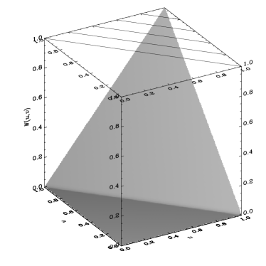
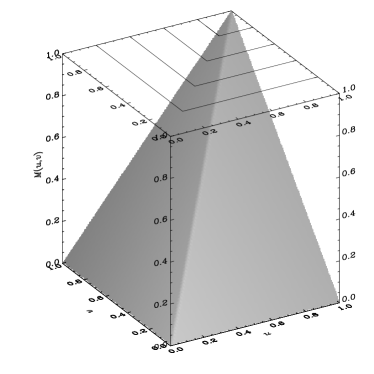
Figure 1: The Fréchet-Hoeffding lower and upper bounds. Left and right panels show the lower and upper bounds, respectively. The top panels represent the contours of $W(u,v))$ and $M(u,v)$.

With these concepts, we now define a two-dimensional copula.

Definition 4

A two-dimensional copula (or shortly 2-copula) is a function $C$ with the following properties:

1. $\mbox{Dom }C=[0,1]\times[0,1]$;

2. $C$ is grounded and 2-increasing;

3. For every $u$ and $v$ in [0,1],

   $$C(u,1)=u\;\mbox{and}\;C(1,v)=v\;.$$ (2)

It may be useful to show there are upper and lower limits for the ranges of copulas, which is given by the following theorem.

Theorem 1

Let $C$ be a copula. Then, for every $(u,v)$ in $\mbox{Dom }C$,

$$\max(u+v-1,0)\leq C(u,v)\leq\min(u,v)\;.$$ (3)

Often the notations $W(u,v)\equiv\max(u+v-1,0)$ and $M(u,v)\equiv\min(u,v)$ are used. The former and the latter are referred to as Fréchet-Hoeffding lower bound and Fréchet-Hoeffding upper bound, respectively.

The Fréchet-Hoeffding lower and upper bounds are illustrated in Fig. 1. Any copula has its value between $W(u,v)$ and $M(u,v)$.

Any bivariate function which satisfies the above conditions can be a copula. Then, there are infinite degrees of freedom for a set of copulas. Using a copula $C$, we can construct a bivariate DF $G$ with two margins $F_{1}$ and $F_{2}$ as

$$G(x_{1},x_{2})=C[F(x_{1}),F_{2}(x_{2})]\;.$$ (4)

However, one may have a natural question: can any bivariate DF be written in the above form? This is guaranteed by Sklar’s theorem (Sklar, 1959).

Theorem 2

(Sklar’s theorem) Let $G$ be a joint distribution function with margins $F_{1}$ and $F_{2}$. Then, there exists a copula $C$ such that for all $x_{1},x_{2}$ in $\bar{\mathbb{R}}$,

$$G(x_{1},x_{2})=C[F_{1}(x_{1}),F_{2}(x_{2})]\;.$$ (5)

If $F_{1}$ and $F_{2}$ are continuous, then $C$ is unique: otherwise, $C$ is uniquely determined on $\mbox{Range }F_{1}\times\mbox{Range }F_{2}$.

A comprehensive proof Sklar’s theorem is found in e.g., Nelsen (2006). This theorem gives a basis that any bivariate DF with given margins is expressed with a form of Equation (5). Then, finally, the somewhat abstract definition of a copula turns out to be really useful for our aim, i.e., to construct a bivariate DF when its marginals are known in some way.

Up to now, we discuss only bivariate DFs and their copulas. It is straightforward to introduce multivariate DFs as a natural extension of the formulation presented here.

2.2 Copulas and dependence measures between two variables

The most important statistical aspect of bivariate DFs is their dependence properties between variables. Since the dependence can never given by the marginals of a DF, this is the most nontrivial information which a bivariate DF provides. Since any bivariate DFs are described by Equation (5), all the information on the dependence is carried by their copulas.

The most familiar measure of dependence among physical scientists (and others) may be the correlation coefficients, especially Pearson’s product-moment correlation coefficient $\rho$. The bivariate PDF of $x_{1}$ and $x_{2}$, $g(x_{1},x_{2})$, is written as

$$g(x_{1},x_{2})=\frac{\partial^{2}C[F_{1}(x_{1}),F_{2}(x_{2})]}{\partial x_{1}\partial x_{2}}f_{1}(x_{1})f_{2}(x_{2})\equiv c[F_{1}(x_{1}),F_{2}(x_{2})]f_{1}(x_{1})f_{2}(x_{2})$$ (6)

where $f_{1}(x_{1})$ and $f_{2}(x_{2})$ are PDF of $F_{1}(x_{1})$ and $F_{2}(x_{2})$, respectively. Then the correlation coefficient is expressed as

$$\rho=\frac{\int(x_{1}-\bar{x_{1}})(x_{2}-\bar{x_{2}})g(x_{1},x_{2}){\rm d}x_{1}{\rm d}x_{2}}{\sqrt{\int(x_{1}-\bar{x_{1}})^{2}f_{1}(x_{1}){\rm d}x_{1}\int(x_{2}-\bar{x_{2}})^{2}f_{2}(x_{2}){\rm d}x_{2}}}=\frac{\int(x_{1}-\bar{x_{1}})(x_{2}-\bar{x_{2}})c[(F_{1}(x_{1}),F_{2}(x_{2})]f_{1}(x_{1})f_{2}(x_{2}){\rm d}x_{1}{\rm d}x_{2}}{\sqrt{\int(x_{1}-\bar{x_{1}})^{2}f_{1}(x_{1}){\rm d}x_{1}\int(x_{2}-\bar{x_{2}})^{2}f_{2}(x_{2}){\rm d}x_{2}}}\;.$$ (7)

We should note that $\rho$ can measure only a linear dependence of two variables. However, in general the dependence of two variables would be not linear at all, and it cannot be a sufficient measure of dependence. Further, more fundamentally, Equation (7) depends not only on the dependence of two variables (copula part) but also its marginals $f_{1}(x_{1}),f_{2}(x_{2})$, i.e., the linear correlation coefficient $\rho$ does not measure the dependence purely. In such a situation, a more flexible and genuine measure of dependence, e.g., Spearman’s $\rho_{\rm S}$ or Kendall’s $\tau$ would be more appropriate. Spearman’s rank correlation is a nonparametric version of Pearson’s correlation using ranked data. The population version of Spearman’s $\rho_{\rm S}$ is expressed by copula as

$$\rho_{\rm S} = 12\int_{0}^{1}\int_{0}^{1}u_{1}u_{2}{\rm d}C(u_{1},u_{2})-3$$ (8)

$$= 12\int_{0}^{1}\int_{0}^{1}C(u_{1},u_{2}){\rm d}u_{1}{\rm d}u_{2}-3\;.$$

The definition of Kendall’s tau is more complicated. We define a concept of concordance as follows: when we have pairs of data $(x_{1i},x_{2i})$ and $(x_{1j},x_{2j})$, they are said to be concordant if $x_{1i}>x_{1j}$ and $x_{2i}>x_{2j}$ or $x_{1i}<x_{1j}$ and $x_{2i}<x_{2j}$ (i.e., $(x_{1i}-x_{1j})(x_{2i}-x_{2j})>0$), and otherwise discordant. Let $\{x_{1i},x_{2i}\}_{i=1,\dots,n}$ denote a random sample of $n$ observations. There are ${}_{n}C_{2}$ pairs $(x_{1i},x_{2i})$ and $(x_{1j},x_{2j})$ of observations in the sample, and each pair is concordant or discordant. Let $n_{\rm c}$ denote the number of concordant pairs, and $n_{\rm d}$ the number of discordant ones. Then, Kendall’s $\tau$ for the sample, $t$, is defined as

$$t=\frac{n_{\rm c}-n_{\rm d}}{n_{\rm c}+n_{\rm d}}\;.$$ (9)

The population version of $\tau$ is also expressed in a simple form in terms of copula as

$$\tau = 4\int_{0}^{1}\int_{0}^{1}C(u_{1},u_{2}){\rm d}C(u_{1},u_{2})-1$$ (10)

$$= 4\int_{0}^{1}\int_{0}^{1}C(u_{1},u_{2})c(u_{1},u_{2}){\rm d}u_{1}{\rm d}u_{2}-1\;.$$

Note that both Equations (8) and (10) are independent of the distributions $F_{1},F_{2}$ and $G$, but they only show the dependence structure described by the copula, unlike the linear correlation coefficient. This is a direct consequence of the non-parametric (i.e., distribution-free) nature of these estimators. These are the reasons why both dependence measures are almost always used in the context of copulas in the literature. Estimators of $\rho_{\rm S}$ and $\tau$ from a sample are found in Appendix B.

2.3 Farlie–Gumbel–Morgenstern (FGM) copula

As seen in the discussion above, usefulness of the linear correlation coefficient is quite limited, and distribution-free measures of dependence are more appropriate for general joint DFs with non-Gaussian marginals. However, even if it is true, since physicists may cling to the most familiar linear correlation coefficient $\rho$, a copula which has an explicit dependence on $\rho$ would be convenient. We introduce two special types of copulas with this ideal property.

For cases where the correlation between two variables is weak, a systematic method has been proposed by Morgenstern (1956) and Gumbel (1960) for specific functional forms, and later generalized to arbitrary functions by Farlie (1960). This is known as the Farlie–Gumbel–Morgenstern (FGM) distributions after the inventors’ names. Although the study of the FGM distributions does not seem tightly connected to that of copulas, we will see later that they can be expressed in terms of the so-called FGM copula.

The correlation structure of the FGM distributions was studied by Schucany, Parr, & Boyer (1978). Let $F_{1}(x_{1})$ and $F_{2}(x_{2})$ be the (cumulative) distribution functions (DFs) of a stochastic variables $x$ and $y$, respectively, and let $f_{1}(x_{1})$ and $f_{2}(x_{2})$ be their probability density functions (PDFs). The bivariate FGM system of distributions $G(x_{1},x_{2})$ is written as

$$G(x_{1},x_{2})=F_{1}(x_{1})F_{2}(x_{2})\left\{1+\kappa\left[1-F_{1}(x_{1})\right]\left[1-F_{2}(x_{2})\right]\right\}\,$$ (11)

where $G(x_{1},x_{2})$ is the joint DF of $x_{1}$ and $x_{2}$. Here $\kappa$ is a parameter related to the correlation (see below), and to make $G(x_{1},x_{2})$ have an appropriate property as a bivariate DF, $\left|\kappa\right|\leq 1$ is required (for a proof, see Cambanis, 1977). Its PDF can be obtained by a direct differentiation of $G(x_{1},x_{2})$ as

$$g(x_{1},x_{2}) \equiv \left.\frac{\partial^{2}G}{\partial x_{1}\partial x_{2}}\right|_{x_{1},x_{2}}=\left.\frac{\partial^{2}}{\partial x_{1}\partial x_{2}}\left\{F_{1}(x_{1})F_{2}(x_{2})\left[1+\kappa\left(1-F_{1}(x_{1})\right)\left(1-F_{2}(x_{2})\right)\right]\right\}\right|_{x_{1},x_{2}}$$ (12)

$$= f_{1}(x_{1})f_{2}(x_{2})\left\{1+\kappa\left[2F_{1}(x_{1})-1\right]\left[2F_{2}(x_{2})-1\right]\right\}\;.$$

From Equation (12), it is straightforward to obtain its covariance function $\mathsf{Cov}(x_{1},x_{2})$ as

$$\mathsf{Cov}(x_{1},x_{2})=\kappa\int x_{1}\left[2F_{1}(x_{1})-1\right]f_{1}(x_{1}){\rm d}x_{1}\int x_{2}\left[2F_{2}(x_{2})-1\right]f_{2}(x_{2}){\rm d}x_{2}\;.$$ (13)

Then we have a correlation function of two stochastic variables $x_{1}$ and $x_{2}$, $\rho(x_{1},x_{2})$ [Equation (7)] as follows

$$\rho(x_{1},x_{2})=\frac{\mathsf{Cov}(x_{1},x_{2})}{\sigma_{1}\sigma_{2}}=\frac{\kappa}{\sigma_{1}\sigma_{2}}\int x_{1}\left[2F_{1}(x_{1})-1\right]f_{1}(x_{1}){\rm d}x_{1}\int x_{2}\left[2F_{2}(x_{2})-1\right]f_{2}(x_{2}){\rm d}x_{2}\;.$$ (14)

where $\sigma_{1}$ and $\sigma_{2}$ are the standard deviations of $x_{1}$ and $x_{2}$ with respect to $f_{1}(x_{1})$ and $f_{2}(x_{2})$. It is straightforwardly confirmed that $g(x_{1},x_{2})$ really has the marginals $f_{1}(x_{1})$ and $f_{2}(x_{2})$, by a direct integration with respect to $x_{1}$ or $x_{2}$. It is also clear that if we want a bivariate PDF with a prescribed correlation coefficient $\rho$, we can determine the parameter $\kappa$ from Equations (7) and (13).

Here, consider the case that that both $f_{1}(x_{1})$ and $f_{2}(x_{2})$ are the Gamma distributions, i.e.,

$$f_{j}(x_{j})=\frac{{x_{j}}^{a-1}e^{-{x_{j}}/b}}{b^{a}\Gamma(a)}$$ (15)

where $\Gamma(x)$ is the gamma function ($j=1,2$). In this case, after some algebra, $\rho$ can be written analytically as

$$\rho(x_{1},x_{2})=\frac{\kappa}{\sqrt{ab}}\left[\frac{2^{-2(a-1)}}{B(a,a)}\right]\left[\frac{2^{-2(b-1)}}{B(b,b)}\right]\;$$ (16)

where

$$B(a,b)\equiv\frac{\Gamma(a)\Gamma(b)}{\Gamma(a+b)}\;.$$ (17)

This result was obtained by D’Este (1981). Especially when $b=1$, this corresponds to a bivariate extension of the Schechter function (Schechter, 1976), and we expect some astrophysical applications.

As we mentioned, the correlation of the FGM distributions is restricted to be weak: indeed, the correlation coefficient cannot exceed $1/3$. Here we prove this. For all (absolutely continuous) $F(x)$,

$$\left\{\int x\left[2F(x)-1\right]f(x){\rm d}x\right\}^{2} = \left\{\int\left(x-\bar{x}\right)\left[2F(x)-1\right]f(x){\rm d}x\right\}^{2}$$ (18)

$$\leq \int\left(x-\bar{x}\right)^{2}f(x){\rm d}x\int\left[2F(x)-1\right]^{2}f(x){\rm d}x=\frac{\sigma^{2}}{3}\;,$$

where $\bar{x}$ is the average of $x$. The second line follows from the Cauchy–Schwarz inequality. From Equations (13) and (7), and the condition $\left|\kappa\right|\leq 1$, we obtain $\left|\rho\right|\leq 1/3$.

The copula of the FGM family of distributions is expressed as

$$C^{\rm FGM}(u_{1},u_{2};\kappa)=u_{1}u_{2}+\kappa u_{1}u_{2}(1-u_{1})(1-u_{2})$$ (19)

with $-1<\kappa<1$. The differential form of the FGM copula follows from Equations (6) and (19)

$$c^{\rm FGM}(u_{1},u_{2};\kappa)=1+\kappa(1-2u_{1})(1-2u_{2})\;.$$ (20)

2.4 Gaussian copula

As seen in Section 2.3, though the FGM distribution has one of the most “natural” example of bivariate DF which has an explicit $\rho$-dependence, the limitation of the correlation coefficient of the FGM family hampers a flexible application of this DF, though there have been many attempts to extend its range of application (see Appendix A). Then, the second natural candidate may be a copula related to a bivariate Gaussian DF. The Gaussian copula has also an explicit dependence on a linear correlation coefficient by its construction.

Let

$$\psi_{1}(x)=\frac{1}{\sqrt{2\pi}}\exp\left(-\frac{x^{2}}{2}\right)\;,$$ (21)

$$\Psi_{1}=\int_{-\infty}^{x}\Psi(x^{\prime}){\rm d}x^{\prime}\;,$$ (22)

$$\psi_{2}(x_{1},x_{2};\rho)=\frac{1}{\sqrt{(2\pi)^{2}(1-\rho^{2})}}\exp\left[-{\frac{x_{1}^{2}+x_{2}^{2}-2\rho x_{1}x_{2}}{2(1-\rho^{2})}}\right]\;,$$ (23)

and

$$\Psi_{2}(x_{1},x_{2};\rho)=\int_{-\infty}^{x_{1}}\int_{-\infty}^{x_{2}}\psi_{i}(x_{1}^{\prime},x_{2}^{\prime}){\rm d}x_{1}^{\prime}{\rm d}x_{2}^{\prime}\;.$$ (24)

By using the covariance matrix ${\mathbf{\Sigma}}$

$${\mathbf{\Sigma}}\equiv\begin{pmatrix}1&\rho\\ \rho&1\end{pmatrix}\;,$$ (25)

Equation (23) is simplified as

$$\psi_{2}(x_{1},x_{2};\rho)=\frac{1}{\sqrt{(2\pi)^{2}\det{\mathbf{\Sigma}}}}\exp\left(-\frac{1}{2}\mathbf{x}^{T}{\mathbf{\Sigma}}^{-1}\mathbf{x}\right)\;,$$ (26)

where $\mathbf{x}\equiv(x_{1},x_{2})^{T}$ and superscript $T$ stands for the transpose of a matrix or vector.

Then, we define a Gaussian copula $C^{\rm G}(u_{1},u_{2};\rho)$ as

$$C^{\rm G}(u_{1},u_{2};\rho)=\Psi_{2}\left[\Psi_{1}^{-1}(u_{1}),\Psi_{1}^{-1}(u_{2});\rho\right]\;.$$ (27)

The density of $C^{\rm G}$, $c^{G}$, is obtained as

$$c^{\rm G}(u_{1},u_{2};\rho) = \frac{\partial^{2}C^{\rm G}(u_{1},u_{2};\rho)}{\partial u_{1}\partial u_{2}}=\frac{\partial^{2}\Psi_{2}\left[\Psi_{1}^{-1}(u_{1}),\Psi_{1}^{-1}(u_{2});\rho\right]}{\partial u_{1}\partial u_{2}}$$ (28)

$$= \frac{\psi_{2}(x_{1},x_{2};\rho)}{\psi_{1}(x_{1})\psi_{1}(x_{2})}$$

$$= \frac{\mathstrut\displaystyle\frac{1}{\sqrt{(2\pi)^{2}\det{\mathbf{\Sigma}}}}\exp\left(-\frac{1}{2}\mathbf{x}^{T}{\mathbf{\Sigma}}^{-1}\mathbf{x}\right)}{\mathstrut\displaystyle\frac{1}{\sqrt{2\pi}}\exp\left(-\frac{x_{1}^{2}}{2}\right)\frac{1}{\sqrt{2\pi}}\exp\left(-\frac{x_{2}^{2}}{2}\right)}$$

$$= \frac{1}{\sqrt{\det{\mathbf{\Sigma}}}}\exp\left[-\frac{1}{2}\left(\mathbf{x}^{T}{\mathbf{\Sigma}}^{-1}\mathbf{x}-\mathbf{x}^{T}{\mathbf{I}}\mathbf{x}\right)\right]$$

$$= \frac{1}{\sqrt{\det{\mathbf{\Sigma}}}}\exp\left\{-\frac{1}{2}\left[\mathbf{x}^{T}\left({\mathbf{\Sigma}}^{-1}-{\mathbf{I}}\right)\mathbf{x}\right]\right\}$$

$$= \frac{1}{\sqrt{\det{\mathbf{\Sigma}}}}\exp\left\{-\frac{1}{2}\left[\mathbf{\Psi^{-1}}^{T}\left({\mathbf{\Sigma}}^{-1}-{\mathbf{I}}\right)\mathbf{\Psi^{-1}}\right]\right\}\;,$$

where $\mathbf{\Psi^{-1}}\equiv\left[\Psi^{-1}(u_{1}),\Psi^{-1}(u_{2})\right]^{T}$ and ${\mathbf{I}}$ stands for the identity matrix. The second line follows from Equation (6).

Figure 2: The bivariate luminosity functions (BLFs) constructed with the Farlie–Gumbel–Morgenstern copula, with model luminosity functions (LFs) of ultraviolet (UV) and infrared (IR)-selected galaxies. The BLFs are normalized so that integrating it over the whole ranges of $L_{1}$ and $L_{2}$ gives one. From top-left to bottom-right, the linear correlation coefficient $\rho=0.0$, 0.1, 0.2, and 0.3, corresponding to $\kappa=0.0,0.33,0.67$ and 1.0, respectively. The contours are logarithmic with an interval $\Delta\log\phi^{(2)}=0.5$ drawn from the peak probability.

3 Application to construct the bivariate luminosity function (BLF) of galaxies

3.1 Construction of the BLF

We define the luminosity at a certain wavelength band by $L\equiv\nu L_{\nu}$ ($\nu$ is the corresponding frequency). Then the luminosity function is defined as a number density of galaxies whose luminosity lies between a logarithmic interval $[\log L,\log L+{\rm d}\log L]$:

$$\phi^{(1)}(L)\equiv\frac{{\rm d}n}{{\rm d}\log L}\;,$$ (29)

where we denote $\log x\equiv\log_{10}x$ and $\ln x\equiv\log_{e}x$. For mathematical simplicity, we define the LF as being normalized, i.e.,

$$\int\phi^{(1)}(L){\rm d}\log L=1\;.$$ (30)

Hence, this corresponds to a probability density function (PDF), a commonly used terminology in the field of mathematical statistics. We also define the cumulative LF as

$$\Phi^{(1)}(L)\equiv\int_{\log L_{\rm min}}^{\log L}\phi^{(1)}(L^{\prime}){\rm d}\log L^{\prime}\;,$$ (31)

where $L_{\rm min}$ is the minimum luminosity of galaxies considered. This corresponds to the DF.

Figure 3: The analytical BLF constructed with the Gaussian copula with model luminosity functions (LFs) of ultraviolet (UV) and infrared (IR)-selected galaxies.. The BLFs are again normalized so that integrating it over the whole ranges of $L_{1}$ and $L_{2}$ gives one. The linear correlation coefficient $\rho$ varies from 0.0 to 0.9 from top-left to bottom-right. The same as Fig. 2, the contours are logarithmic with an interval $\Delta\log\phi^{(2)}=0.5$ drawn from the peak probability.

If we denote univariate LFs as $\phi^{(1)}_{1}(L_{1})$ and $\phi^{(1)}_{2}(L_{2})$, then the bivariate PDF $\phi^{(2)}(L_{1},L_{2})$ is described by a differential copula $c(u_{1},u_{2})$ as

$$\phi^{(2)}(L_{1},L_{2}) \equiv c\left[\phi^{(1)}_{1}(L_{1}),\phi^{(1)}_{2}(L_{2})\right]\;.$$ (32)

For the FGM copula, the BLF leads from Equation (20)

$$\phi^{(2)}(L_{1},L_{2};\kappa) \equiv \left\{1+\kappa\left[2\Phi^{(1)}_{1}(L_{1})-1\right]\left[2\Phi^{(1)}_{2}(L_{2})-1\right]\right\}\phi^{(1)}_{1}(L_{1})\phi^{(1)}_{2}(L_{2})\;.$$ (33)

The parameter $\kappa$ is proportional to the correlation coefficient $\rho$ between $\log L_{1}$ and $\log L_{2}$. For the Gaussian copula, the BLF is obtained as

$$\phi^{(2)}(L_{1},L_{2};\rho) = \frac{1}{\sqrt{\det{\mathbf{\Sigma}}}}\exp\left\{-\frac{1}{2}\left[\mathbf{\Psi^{-1}}^{T}\left({\mathbf{\Sigma}}^{-1}-{\mathbf{I}}\right)\mathbf{\Psi^{-1}}\right]\right\}\phi^{(1)}_{1}(L_{1})\phi^{(1)}_{2}(L_{2})\;,$$ (34)

where

$$\mathbf{\Psi^{-1}}=\left[\Psi^{-1}\left(\Phi^{(1)}_{1}(L_{1})\right),\;\Psi^{-1}\left(\Phi^{(1)}_{2}(L_{2})\right)\right]^{T}$$ (35)

and ${\mathbf{\Sigma}}$ is again defined by Equation (25).

3.2 The FIR-FUV BLF

Here, to make our model BLF astrophysically realistic, we construct the FUV–FIR BLF by the copula method. For the IR, we use the analytic form for the LF proposed by Saunders et al. (1990) which is defined as

$$\phi^{(1)}_{1}(L)=\phi_{*1}\left(\frac{L}{L_{*1}}\right)^{1-\alpha_{1}}\exp\left\{-\frac{1}{2\sigma^{2}}\left[\log\left(1+\frac{L}{L_{*1}}\right)\right]^{2}\right\}\;.$$ (36)

We adopt the parameters estimated by (Takeuchi et al.2003b) which are obtained from the IRAS PSC$z$ galaxies (Saunders et al., 2000). For the UV, we adopt the Schechter function (Schechter, 1976).

$$\phi^{(1)}_{2}(L)=(\ln 10)\;\phi_{*2}\left(\frac{L}{L_{*2}}\right)^{1-\alpha_{2}}\exp\left[-\left(\frac{L}{L_{*2}}\right)\right]\;,$$ (37)

We use the parameters presented by Wyder et al. (2005) for GALEX FUV ($\lambda_{\rm eff}=1530\;$Å): $(\alpha_{2},L_{*2},\phi_{*2})=(1.21,1.81\times 10^{9}h^{-2}\;L_{\odot},1.35\times 10^{-2}h^{3}\;\mbox{Mpc}^{-3})$. For simplicity, we neglect the $K$-correction. We use the re-normalized version of Eqs. (36) and (37) so that they can be regarded as PDFs, as mentioned above.

3.3 Result

We show the constructed BLFs from the FGM and Gaussian copulas in Figures 2 and 3, respectively. The FGM-based BLF cannot have a linear correlation coefficient larger than $\simeq 0.3$ as explained above, while the Gaussian-based BLF may have a much higher linear correlation. We note that both copulas allow negative correlations, which are not discussed in this article.

First, even if the linear correlation coefficients are the same, the detailed structures of the BLFs with the FGM and Gaussian copulas are different (see the case of $\rho=0.0\mbox{--}0.3$). For the Gaussian-based BLFs, we see a decline at the faint end, while we do not have such structure in the FGM-based BLFs (see the closed contours in Fig. 3). This structure is introduced by the Gaussian copula, and from the physical point of view, it might not be strongly desired. The FGM-based BLF has a more ideal shape.

Second, since the univariate LF shapes are different at FIR and FUV, the ridge of the BLF is not a straight line but clearly nonlinear. This feature is more clearly visible in higher correlation cases in Figure 3, but always exists for the whole range of $\rho$. This trend is indeed found in the $L_{\rm FIR}$–$L_{\rm FUV}$ diagram (Martin et al., 2005). The underlying physics is that galaxies with high SFRs are more extinguished by dust (e.g. Buat et al., 2007a, b).

Observational applications including this topic will be presented elsewhere (Takeuchi et al. 2010, in preparation).

4 Discussion

4.1 Flux selection effect in multiband surveys

Since we have an explicit form of a BLF, we can discuss the flux selection effect formally. For simplicity, we consider the bivariate case (i.e. sample selected at two bands), but it will be straightforward to extend the formulation to a multiwavelength case (or more generally, selected using any physical properties). The flux selection is described in terms of luminosity as putting a lower bound $L^{\rm lim}$ on a luminosity–luminosity ($L_{1}$–$L_{2}$) plane. The lower bound luminosity $L^{\rm lim}$ is defined by the flux (density) detection limit $S^{\rm lim}$ as a function of redshift. In most surveys, a certain wavelength band is chosen as the primary selection band, like B-band, Ks-band, $60\;\mu$m-selected, etc. The schematic description of a survey is presented in Figure 4.

If we select a sample of objects (in our case galaxies) at band 1, the objects with $L_{1}<L^{\rm lim}_{1}(z)$ would not be included in the sample at a certain redshift $z$. Then, the detected sources should have $L_{1}>L^{\rm lim}_{1}(z)$ and $L_{2}>L^{\rm lim}_{2}(z)$. Hence, on the $L_{1}$–$L_{2}$ plane, the 2-dim distribution of the detected objects is expressed as

$$\Sigma^{\rm det}(L_{1},L_{2})\equiv\int_{0}^{z}\frac{\displaystyle{\rm d}^{2}V}{{\rm d}z^{\prime}{\rm d}\Omega}\phi^{(2)}\left(L_{1},L_{2}\right)\Theta\left(L^{\rm lim}_{1}(z^{\prime})\right)\Theta\left(L^{\rm lim}_{2}(z^{\prime})\right){\rm d}z^{\prime}\;,$$ (38)

where $\Omega$ is a solid angle, and $\Theta$ is the Heaviside step function defined as

$$\Theta(a)=\begin{cases}0&L<a\\ 1&L\geq a\end{cases}\;.$$ (39)

The quantity $\Sigma^{\rm det}$ is proportional to the surface number density of objects detected in both bands on the $L_{1}$–$L_{2}$ plane. We start from a primary selection at band 1, then we would have objects detected at band 1 but not detected at band 2. In such a case we only have upper limits for these objects. The 2-dim distribution of the upper limits at band 2 is similarly formulated as

$$\Sigma^{\rm UL2}(L_{1},L_{2})\equiv\int_{0}^{z}\frac{\displaystyle{\rm d}^{2}V}{{\rm d}z^{\prime}{\rm d}\Omega}\phi^{(2)}\left(L_{1},L_{2}\right)\Theta\left(L^{\rm lim}_{1}(z^{\prime})\right)\left[1-\Theta\left(L^{\rm lim}_{2}(z^{\prime})\right)\right]{\rm d}z^{\prime}\;.$$ (40)

The superscript UL2 stands for “upper limit at band 2”. In statistical terminology, the upper limit case, i.e. we know there is an object but we do only have the upper (or lower) limits of a certain quantity, is referred to as “censored”. Though we can define the distribution $\Sigma^{\rm UL2}(L_{1},L_{2})$ by Eq. (40), since the sample objects belonging to this category appear only as upper limits on the plot, a special statistical treatment, referred to as the survival analysis, is required to estimate $\Sigma^{\rm UL2}(L_{1},L_{2})$ from the data. Since we select objects at band 1, we do not have upper limits at band 1, because we do not know if there would be an object below the limit. This case is called “truncated” in statistics.

If we select objects at band 2, we can formulate the 2-dim distribution of detected objects and upper limits exactly in the same way as the band 1 selected sample. For the objects detected at both bands, the 2-dim distribution is expressed by Eq. (38). The objects detected at band 2 but not detected at band 1 is expressed as

$$\Sigma^{\rm UL1}(L_{1},L_{2})\equiv\int_{0}^{z}\frac{\displaystyle{\rm d}^{2}V}{{\rm d}z^{\prime}{\rm d}\Omega}\phi^{(2)}\left(L_{1},L_{2}\right)\left[1-\Theta\left(L^{\rm lim}_{1}(z^{\prime})\right)\right]\Theta\left(L^{\rm lim}_{2}(z^{\prime})\right){\rm d}z^{\prime}\;.$$ (41)

If we can model $L^{\rm lim}_{1}(z)$ and $L^{\rm lim}_{2}(z)$ precisely including the $K$-correction, evolutionary effect, etc., we can use the observed bivariate luminosity distribution to estimate the correlation coefficient, or more generally the dependence structure of two luminosities through Eqs. (38)–(40). We can deal with these cases in a unified manner with techniques developed in survival analysis. We discuss this issue in a subsequent work (Takeuchi et al. 2010, in preparation).

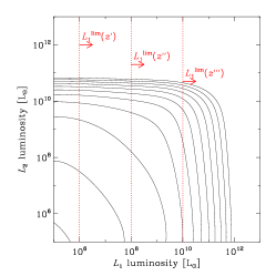
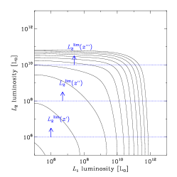
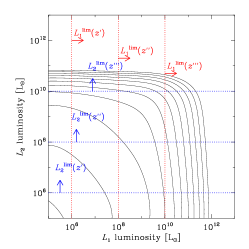
Figure 4: Schematic description of the selection effect in a multiband survey. Left: selection at band 1, center: selection at band 2, and right: bivariate selection at band 1 and 2.

4.2 Other possible applications

4.2.1 The star formation rate function

The star formation rate (SFR) is one of the most fundamental quantities to investigate the formation and evolution of galaxies. The SFR is often estimated from the FUV flux of galaxies (or other related observables like H$\alpha$ etc.) after “correcting” the dust extinction. However, some problems have been pointed out for this method. For instance, the relation between the UV slope $\beta$ (or equivalently, FUV$-$NUV color) and the FIR-FUV flux ratio $L_{\rm FIR}/L_{\rm FUV}$ (often referred to as the IRX-$\beta$ relation) is frequently used to correct the extinction, but this relation is not always the same for various categories of star-forming galaxies (e.g. Buat et al., 2005; Boissier et al., 2007; Boquien et al., 2009; Takeuchi et al., 2010a).

Instead, the total SFR obtained from the FUV and FIR luminosities would be a more reliable measure of the SFR since both are directly observable values (e.g. Iglesias-Páramo et al., 2004; Buat et al., 2005; Iglesias-Páramo et al., 2006; Buat et al., 2007a, b; Takeuchi et al., 2010a). Assuming a constant SFR over $10^{8}\mbox{yr}$, and Salpeter initial mass function (Salpeter, 1955, mass range: $0.1\mbox{--}100\;M_{\odot}$), we have the relation between the SFR and $L_{\rm FUV}$

$$\log\mbox{SFR}_{\rm FUV}=\log L_{\rm FUV}-9.51\;.$$ (42)

For the FIR, to transform the dust emission to the SFR, we assume that all the stellar light is absorbed by dust. Then, we obtain the following formula under the same assumption for both the SFR history and the IMF as those of the FUV,

$$\log\mbox{SFR}_{\rm dust}=\log L_{\rm TIR}-9.75-\log(1-\eta)\;.$$ (43)

Here, $\eta$ is the fraction of the dust emission by old stars which is not related to the current SFR (Hirashita, Buat, & Inoue, 2003), and $L_{\rm TIR}$ is the FIR luminosity integrated over $\lambda=8\mbox{--}1000\;\mu$m. Thus, the total SFR is simply

$$\mbox{SFR}_{\rm tot}=\mbox{SFR}_{\rm FUV}+\mbox{SFR}_{\rm dust}$$ (44)

(Iglesias-Páramo et al., 2006). Since the total SFR is basically estimated from the luminosities at FUV and FIR (note that $\mbox{SFR}_{\rm FUV}\propto L_{\rm FUV}$ and $\mbox{SFR}_{\rm dust}\propto L_{\rm TIR}$), the estimation of the PDF of the total SFR reduces to the estimation of the FIR-FUV BLF (e.g. Takeuchi et al., 2010b). However, since the total SFR is the sum of two dependent variables, it is not straightforward to formulate the function unlike the cases we have seen above. This analysis will be discussed with a more specific methodology in our future work.

4.2.2 The distribution of the specific star formation rate

Another direct application is the distribution of the specific SFR (SSFR), $\mbox{SFR}/M_{*}$ where $M_{*}$ is the total stellar mass of a galaxy. The SSFR has gained much attention in the last decade, since the relation between $M_{*}$ and the SSFR of galaxies turns out to be a very important clue to understand the SF history of galaxies: more massive galaxies have ceased their SF activity earlier in the cosmic time than less massive galaxies (downsizing in redshift: e.g. Cowie et al., 1996; Boselli et al., 2001; Heavens et al., 2004; Feulner et al., 2005; Noeske et al., 2007a, b; Panter et al., 2007; Damen et al., 2009a, b, among others). For a comprehensive summary of the downsizing, readers are encouraged to read Introduction of Fontanot et al. (2009). Despite of its importance, the treatment of multiwavelength data for this analysis is inevitably complicated and does not seem to be well understood, because we must deal with the data related to SFR and $M_{*}$ estimation. This might be, at least partially, the reason why the quantitative values of the $M_{*}$–SSFR relation are different among different studies.

As may easily guess after the above discussions, the $M_{*}$–SSFR relation can be reduced to the relation between a luminosity at a certain mass-related band (often near IR bands) and a SF-related one (FUV, FIR, etc.) Then, we can model, for example, a $L_{K}$–$L_{\rm TIR}$ bivariate luminosity function ($L_{K}$: K-band luminosity) to examine the observed relation including all the selection effects. This is particularly useful for this topic, since Takeuchi et al. (2010b) found that the SFRF cannot be described by the Schechter function unlike the assumptions adopted in previous studies, but much more similar to the Saunders IR LF [Eq. (36)]. The selection effect would be more complicated than in the case of the same Schechter marginals, but can be treated in the same way as discussed above. Thus, this may also be an interesting application of the copula-based BLF in the epoch of future large surveys.

5 Summary and Conclusions

In this work, we introduced an analytic method to construct a bivariate distribution function (DF) with given marginal distributions and correlation coefficient, by making use of a convenient mathematical tool, called a copula. Using this mathematical tool, we presented an application to construct a bivariate LF of galaxies (BLF). Specifically, we focused on the FUV–FIR BLF, since these two luminosities are related to the star formation (SF) activity. Though both the FUV and FIR are related to the SF activity, the marginal univariate LFs have a very different functional form: former is well described by Schechter function whilst the latter has a much more extended power-law like luminous end. We constructed the FUV-FIR BLFs by the FGM and Gaussian copulas with different strength of correlation, and examined their statistical properties. Then, we discussed some further possible applications of the BLF: the problem of a multiband flux-limited sample selection, the construction of the SF rate (SFR) function, and the construction of the stellar mass of galaxies ($M_{*}$)–specific SFR ($\mbox{SFR}/M_{*}$) relation.

We summarize our conclusions as follows:

1. If the correlation of two variables is weak (Pearson’s correlation coefficient $|\rho|<1/3$), the Farlie-Gumbel-Morgenstern (FGM) copula provides an intuitive and natural way for constructing such a bivariate DF.

2. When the linear correlation is stronger, the FGM copula becomes inadequate, in which case a Gaussian copula should be preferred. The latter connects two marginals and is directly related to the linear correlation coefficient between two variables.

3. Even if the linear correlation coefficient is the same, the structure of a BLF is different depending on the choice of a copula. Hence, a proper copula should be chosen for each case.

4. The model FIR-FUV BLF was constructed. Since the functional shape of the LF at each wavelength is very different, the obtained BLF has a clear nonlinear structure. This feature was indeed found in actual observational data (e.g., Martin et al., 2005).

5. We formulated the problem of the multiwavelength selection effect by the BLF. This enables us to deal with datasets derived from surveys presenting complex selection functions.

6. We discussed the estimation of the SFR function (SFRF) of galaxies. The copula-based BLF will be a convenient tool to extract detailed information from the observationally estimated SFRF because of its bivariate nature.

7. The stellar mass–specific SFR relation was also discussed. This relation can be reduced to a BLF of luminosities at a mass-related band and a SF-related band. With an analytic BLF model constructed by a copula will provide us with a powerful tool to analyze the downsizing phenomenon with addressing the complicated selection effects.

As the copula becomes better known to the astrophysical community and statisticians develop the copula functions, we envision many more interesting applications in the future. In a series of forthcoming papers, we will present more observationally-oriented applications of copulas.

Appendix A An extension of the FGM system by Johnson & Kotz (1977)

Although the FGM system of distributions provides us with convenient tool to construct the statistical model, its usefulness is restricted by the limitation of the correlation strength described above. To overcome this drawback, many attempts have been made to extend the FGM distributions (see, e.g., , Stuart et al.1994; Kotz, Balakrishnan, & Johnson, 2000). Among them, Johnson & Kotz (1977) introduced the following iterated generalization of Equation (11):

$$G(x_{1},x_{2})=\sum_{j=0}^{k}\kappa_{j}\left[F_{1}(x_{1})F_{2}(x_{2})\right]^{[j/2]+1}\left\{\left[1-F_{1}(x_{1})\right]\left[1-F_{2}(x_{2})\right]\right\}^{[(j+1)/2]}\;,$$ (45)

where the symbol in the exponent $[j/2]$ means the maximum natural number which does not exceed $j/2$. We set $\kappa_{0}=1$. Huang & Kotz (1984) examined the dependence structure of Equation (45) especially for the case of $k=2$, and showed that the correlation can be stronger for these extension. In the case of the one-iteration family ($k=2$), we have the DF as

$$G(x_{1},x_{2})=F_{1}(x_{1})F_{2}(x_{2})\left\{1+\kappa_{1}\left[1-F_{1}(x_{1})\right]\left[1-F_{2}(x_{2})\right]+\kappa_{2}F_{1}(x_{1})F_{2}(x_{2})\left[1-F_{1}(x_{1})\right]\left[1-F_{2}(x_{2})\right]\right\}\;.$$ (46)

The corresponding PDF is

$$g(x_{1},x_{2})=f_{1}(x_{1})f_{2}(x_{2})\left\{1+\kappa_{1}\left[2F_{1}(x_{1})-1\right]\left[2F_{2}(x_{2})-1\right]+\kappa_{2}F_{1}(x_{1})F_{2}(x_{2})\left[3F_{1}(x_{1})-2\right]\left[3F_{2}(x_{2})-2\right]\right\}\;.$$ (47)

Then, just the same as the case of the original FGM distribution ($k=1$), we obtain the covariance

$$\mathsf{Cov}(x_{1},x_{2}) = \iint(x_{1}-\bar{x}_{1})(x_{2}-\bar{x}_{2})f_{1}(x_{1})f_{2}(x_{2})$$ (48)

$$\times\left\{1+\kappa_{1}\left[2F_{1}(x_{1})-1\right]\left[2F_{2}(x_{2})-1\right]+\kappa_{2}F_{1}(x_{1})F_{2}(x_{2})\left[3F_{1}(x_{1})-2\right]\left[3F_{2}(x_{2})-2\right]\right\}dx_{1}dx_{2}$$

$$= \kappa_{1}\int x_{1}f_{1}(x_{1})\left[2F_{1}(x_{1})-1\right]dx_{1}\int x_{2}f_{2}(x_{2})\left[2F_{2}(x_{2})-1\right]dx_{2}$$

$$+\kappa_{2}\int x_{1}f_{1}(x_{1})F_{1}(x_{1})\left[3F_{1}(x_{1})-2\right]dx_{1}\int x_{2}f_{2}(x_{2})F_{2}(x_{2})\left[3F_{2}(x_{2})-2\right]dx_{2}$$

$$\equiv A_{1}\kappa_{1}+A_{2}\kappa_{2}\;.$$

Huang & Kotz (1984) obtained the parameter space for $\kappa_{1}$ and $\kappa_{2}$ as

$$\left|\kappa_{1}\right|\leq 1\;,$$ (49)

$$\kappa_{1}+\kappa_{2}\geq-1\;,$$ (50)

$$\kappa_{2}\leq\frac{3-\kappa_{1}+\sqrt{3(1-\kappa_{1})(3+\kappa_{1})}}{2}\;.$$ (51)

They showed that, for a positive correlation,

$$\rho\leq\frac{\kappa_{1}}{3}+\frac{31\kappa_{2}}{240}\;.$$ (52)

Under these conditions, we have $\rho\leq 0.5072$, which is considerably better than $1/3$. The BLF constructed with the first-order iterated FGM copula is expressed as

$$\phi^{(2)}(L_{1},L_{2}) = \phi^{(1)}_{1}(L_{1})\phi^{(1)}_{2}(L_{2})$$ (53)

$$\times\left\{1+\kappa_{1}\left[2\Phi^{(1)}_{1}(L_{1})-1\right]\left[2\Phi^{(1)}_{2}(L_{2})-1\right]+\kappa_{2}\phi^{(1)}_{1}(L_{1})\phi^{(1)}_{2}(L_{2})\left[3\Phi^{(1)}_{1}(L_{1})-2\right]\left[3\Phi^{(1)}_{2}(L_{2})-2\right]\right\}\;.$$

The FIR-FUV BLF by Equation 53 is shown in Figure 5. Clearly the dependence between the two luminosities is stronger than the original FGM-based BLF. However, now it is not intuitive nor straightforward to relate these two parameters of dependence $\kappa_{1}$ and $\kappa_{2}$ to the linear correlation coefficient.

Figure 5: The BLF constructed with a first-order iterated FGM copula. The linear correlation coefficient $\rho$ is 0.45.

Appendix B Estimators of the nonparametric dependence measures $\rho_{\rm S}$ and $\tau$

Here we present the estimators of the nonparametric measure of dependence introduced in Section 2.2. More detailed derivation and properties of these nonparametric measures of dependence are found in e.g., Hettmansperger (1984) and Hollander & Wolfe (1999).

Let $\{R_{i}\}_{i=1,\dots,n}$ and $\{S_{i}\}_{i=1,\dots,n}$ be the ranks of $\{x_{1i}\}_{i=1,\dots,n}$ and $\{x_{2i}\}_{i=1,\dots,n}$, respectively. If we denote the estimator of $\rho_{\rm S}$ for a sample as $r_{\rm S}$,

$$r_{\rm S}=\frac{\mathstrut\sum_{i=1}^{n}\left(R_{i}-\frac{n+1}{2}\right)\left(S_{i}-\frac{n+1}{2}\right)}{\mathstrut\sqrt{\sum_{i=1}^{n}\left(R_{i}-\frac{n+1}{2}\right)\sum_{i=1}^{n}\left(S_{i}-\frac{n+1}{2}\right)}}\;.$$ (54)

This is also expressed as

$$r_{\rm S}=\frac{\mathstrut 12\sum_{i=1}^{n}\left(R_{i}-\frac{n+1}{2}\right)\left(S_{i}-\frac{n+1}{2}\right)}{\mathstrut n(n^{2}-1)}\;.$$ (55)

This form is an exact sample counterpart of Equation (8). If we define $d_{i}\equiv S_{i}-R_{i}$, Equation (55) reduces to the following simper form

$$r_{\rm S}=1-\frac{\mathstrut 6\sum_{i=1}^{n}d_{i}^{2}}{\mathstrut n(n^{2}-1)}\;.$$ (56)

The variance of $r_{\rm S}$ in the large-sample limit is given by

$$\mathsf{Var}[r_{\rm S}]=\frac{1}{n-1}\;.$$ (57)

The most basic form of Kendall’s $\tau$ for a sample has been already shown in Section 2.2 [Equation (9)]. It is also expressed as

$$t = \frac{\mathstrut 2(n_{\rm c}-n_{\rm d})}{\mathstrut n(n-1)}$$ (58)

$$= 1-\frac{\mathstrut 4}{\mathstrut n(n-1)}n_{\rm d}$$

since $n_{\rm c}+n_{\rm d}=n(n-1)/2$. The variance of $t$ is given by

$$\mathsf{Var}[t]=\frac{2(2n+5)}{9n(n-1)}$$ (59)

(see Valz & Mcleod, 1990, for a very concise derivation).

References

- Ball et al. (2006) Ball N. M., Loveday J., Brunner R. J., Baldry I. K., Brinkmann J., 2006, MNRAS, 373, 845
- Binggeli, Sandage, & Tammann (1988) Binggeli B., Sandage A., Tammann G. A., 1988, ARA&A, 26, 509
- Blanton et al. (2001) Blanton M. R., et al., 2001, AJ, 121, 2358
- Benabed et al. (2009) Benabed K., Cardoso J.-F., Prunet S., Hivon E., 2009, MNRAS, 400, 219
- Boissier et al. (2007) Boissier S., et al., 2007, ApJS, 173, 524
- Boquien et al. (2009) Boquien M., et al., 2009, ApJ, 706, 553
- Boselli et al. (2001) Boselli A., Gavazzi G., Donas J., Scodeggio M., 2001, AJ, 121, 753
- Buat & Burgarella (1998) Buat V., Burgarella D., 1998, A&A, 334, 772
- Buat et al. (2005) Buat V., et al., 2005, ApJ, 619, L51
- Buat et al. (2007a) Buat V., et al., 2007a, ApJS, 173, 404
- Buat et al. (2007b) Buat V., Marcillac D., Burgarella D., Le Floc’h E., Takeuchi T. T., Iglesias-Páramo J., Xu C. K., 2007b, A&A, 469, 19
- Buat et al. (2008) Buat V., et al., 2008, A&A, 483, 107
- Buat et al. (2009) Buat V., Takeuchi T. T., Burgarella D., Giovannoli E., Murata K. L., 2009, A&A, 507, 693
- Cambanis (1977) Cambanis S., 1977, J. Multivariate Analysis, 7. 551
- Chapman et al. (2003) Chapman S. C., Helou G., Lewis G. F., Dale D. A., 2003, ApJ, 588, 186
- Chołoniewski (1985) Chołoniewski J., 1985, MNRAS, 214, 197
- Cowie et al. (1996) Cowie L. L., Songaila A., Hu E. M., Cohen J. G., 1996, AJ, 112, 839
- Cross & Driver (2002) Cross N., Driver S. P., 2002, MNRAS, 329, 579
- Damen et al. (2009a) Damen M., Labbé I., Franx M., van Dokkum P. G., Taylor E. N., Gawiser E. J., 2009a, ApJ, 690, 937
- Damen et al. (2009b) Damen M., Förster Schreiber N. M., Franx M., Labbé I., Toft S., van Dokkum P. G., Wuyts S., 2009b, ApJ, 705, 617
- de Lapparent et al. (2003) de Lapparent V., Galaz G., Bardelli S., Arnouts S., 2003, A&A, 404, 831
- D’Este (1981) D’Este G. M., 1981, Biometrika, 68, 339
- Driver et al. (2006) Driver S. P., et al., 2006, MNRAS, 368, 414
- Farlie (1960) Farlie D. J. G., 1960, Biometrika, 47, 307
- Feulner et al. (2005) Feulner G., Gabasch A., Salvato M., Drory N., Hopp U., Bender R., 2005, ApJ, 633, L9
- Fontanot et al. (2009) Fontanot F., De Lucia G., Monaco P., Somerville R. S., Santini P., 2009, MNRAS, 397, 1776
- Gumbel (1960) Gumbel E. J., 1960, J. Amer. Statist. Assoc., 55, 698
- Heavens et al. (2004) Heavens A., Panter B., Jimenez R., Dunlop J., 2004, Natur, 428, 625
- Hettmansperger (1984) Hettmansperger T. P., 1984, Statistical Inference Based on Ranks, John Wiley & Sons, New York
- Hirashita, Buat, & Inoue (2003) Hirashita H., Buat V., Inoue A. K., 2003, A&A, 410, 83
- Hollander & Wolfe (1999) Hollander M., & Wolfe D. A., 1999, Nonparametric Statistical Methods, 2nd ed., John Wiley & Sons, New York
- Huang & Kotz (1984) Huang J. S., Kotz S., 1984, Biometrika, 71, 633