Limit theorem for a time-dependent
coined quantum walk on the line

Abstract

We study time-dependent discrete-time quantum walks on the one-dimensional lattice. We compute the limit distribution of a two-period quantum walk defined by two orthogonal matrices. For the symmetric case, the distribution is determined by one of two matrices. Moreover, limit theorems for two special cases are presented.

1 Introduction

The discrete-time quantum walk (QW) was first intensively studied by Ambainis et al. [1]. The QW is considered as a quantum generalization of the classical random walk. The random walker in position $x\in\mathbb{Z}=\left\{\,0,\pm 1,\pm 2,\ldots\,\right\}$ at time $t\left(\in\left\{\,0,1,2,\ldots\,\right\}\right)$ moves to $x-1$ at time $t+1$ with probability $p$, or $x+1$ with probability $q\,(\,=1-p)$. In contrast, the evolution of the quantum walker is defined by replacing $p$ and $q$ with $2\times 2$ matrices $P$ and $Q$, respectively. Note that $U=P+Q$ is a unitary matrix. A main difference between the classical walk and the QW is seen on the particle spreading. Let $\sigma(t)$ be the standard deviation of the walk at time $t$. That is, $\sigma(t)=\sqrt{\mathbb{E}(X_{t}^{2})-\mathbb{E}(X_{t})^{2}}$, where $X_{t}$ is the position of the quantum walker at time $t$ and $\mathbb{E}(Y)$ denotes the expected value of $Y$. Then the classical case is a diffusive behavior, $\sigma(t)\sim\sqrt{t}$, while the quantum case is ballistic, $\sigma(t)\sim t$ (see [1], for example).

In the context of quantum computation, the QW is applied to several quantum algorithms. By using the quantum algorithm, we solve a problem quadratically faster than the corresponding classical algorithm. As a well-known quantum search algorithm, Grover’s algorithm was presented. The algorithm solves the following problem: in a search space of $N$ vertices, one can find a marked vertex. The corresponding classical search requires $O(N)$ queries. However, the search needs only $O(\sqrt{N})$ queries. As well as the Grover algorithm, the QW can also search a marked vertex with a quadratic speed up, see Shenvi et al. [2]. It has been reported that quantum walks on regular graphs (e.g., lattice, hypercube, complete graph) give faster searching than classical walks. The Grover search algorithm can also be interpreted as a QW on complete graph. Decoherence is an important concept in quantum information processing. In fact, decoherence on QWs has been extensively investigated, see Kendon [3], for example. However, we should note that our results are not related to the decoherence in QWs. Physically, Oka et al. [4] pointed out that the Landau-Zener transition dynamics can be mapped to a QW and showed the localization of the wave functions.

In the present paper, we consider the QW whose dynamics is determined by a sequence of time-dependent matrices, $\left\{U_{t}:t=0,1,\ldots\right\}$. Ribeiro et al. [5] numerically showed that periodic sequence is ballistic, random sequence is diffusive, and Fibonacci sequence is sub-ballistic. Mackay et al. [6] and Ribeiro et al. [5] investigated some random sequences and reported that the probability distribution of the QW converges to a binomial distribution by averaging over many trials by numerical simulations. Konno [7] proved their results by using a path counting method. By comparing with a position-dependent QW introduced by Wójcik et al. [8], Bañuls et al. [9] discussed a dynamical localization of the corresponding time-dependent QW.

In this paper, we present the weak limit theorem for the two-period time-dependent QW whose unitary matrix $U_{t}$ is an orthogonal matrix. Our approach is based on the Fourier transform method introduced by Grimmett et al. [10]. We think that it would be difficult to calculate the limit distribution for the general $n$-period ($n=3,4,\ldots$) walk. However, we find out a class of time-dependent QWs whose limit probability distributions result in that of the usual (i.e., one-period) QW. As for the position-dependent QW, a similar result can be found in Konno [11].

The present paper is organized as follows. In Sect. 2, we define the time-dependent QW. Section 3 treats the two-period time-dependent QW. By using the Fourier transform, we obtain the limit distribution. Finally, in Sect. 4, we consider two special cases of time-dependent QWs. We show that the limit distribution of the walk is the same as that of the usual one.

2 Time-dependent QW

In this section we define the time-dependent QWs. Let $\ket{x}$ ($x\in\mathbb{Z}$) be infinite components vector which denotes the position of the walker. Here, $x$-th component of $\ket{x}$ is 1 and the other is 0. Let $\ket{\psi_{t}(x)}\in\mathbb{C}^{2}$ be the amplitude of the walker in position $x$ at time $t$, where $\mathbb{C}$ is the set of complex numbers. The time-dependent QW at time $t$ is expressed by

$$\ket{\Psi_{t}}=\sum_{x\in\mathbb{Z}}\ket{x}\otimes\ket{\psi_{t}(x)}.$$ (1)

To define the time evolution of the walker, we introduce a unitary matrix

$$U_{t}=\left[\begin{array}[]{cc}a_{t}&b_{t}\\ c_{t}&d_{t}\end{array}\right],$$ (2)

where $a_{t},b_{t},c_{t},d_{t}\,\in\mathbb{C}$ and $a_{t}b_{t}c_{t}d_{t}\neq 0\,\,(t=0,1,\ldots)$. Then $U_{t}$ is divided into $P_{t}$ and $Q_{t}$ as follows:

$$P_{t}=\left[\begin{array}[]{cc}a_{t}&b_{t}\\ 0&0\end{array}\right],\,Q_{t}=\left[\begin{array}[]{cc}0&0\\ c_{t}&d_{t}\end{array}\right].$$ (3)

The evolution is determined by

$$\ket{\Psi_{t+1}}=\sum_{x\in\mathbb{Z}}\ket{x}\otimes\left(P_{t}\ket{\psi_{t}(x+1)}+Q_{t}\ket{\psi_{t}(x-1)}\right).$$ (4)

Let $||\ket{y}||^{2}=\braket{y}{y}$. The probability that the quantum walker $X_{t}$ is in position $x$ at time $t$, $P(X_{t}=x)$, is defined by

$$P(X_{t}=x)=||\ket{\psi_{t}(x)}||^{2}.$$ (5)

Moreover, the Fourier transform $\ket{\hat{\Psi}_{t}(k)}\,(k\in\left[0,2\pi\right))$ is given by

$$\ket{\hat{\Psi}_{t}(k)}=\sum_{x\in\mathbb{Z}}e^{-ikx}\ket{\psi_{t}(x)},$$ (6)

with $i=\sqrt{-1}$. By the inverse Fourier transform, we have

$$\ket{\psi_{t}(x)}=\int_{0}^{2\pi}\frac{dk}{2\pi}e^{ikx}\ket{\hat{\Psi}_{t}(k)}.$$ (7)

The time evolution of $\ket{\hat{\Psi}_{t}(k)}$ is

$$\ket{\hat{\Psi}_{t+1}(k)}=\hat{U}_{t}(k)\ket{\hat{\Psi}_{t}(k)},$$ (8)

where $\hat{U}_{t}(k)=R(k)U_{t}$ and $R(k)=\left[\begin{array}[]{cc}e^{ik}&0\\ 0&e^{-ik}\end{array}\right]$. We should remark that $R(k)$ satisfies $R(k_{1})R(k_{2})=R(k_{1}+k_{2})$ and $R(k)^{\ast}=R(-k)$, where $\ast$ denotes the conjugate transposed operator. From (8), we see that

$$\ket{\hat{\Psi}_{t}(k)}=\hat{U}_{t-1}(k)\hat{U}_{t-2}(k)\cdots\hat{U}_{0}(k)\ket{\hat{\Psi}_{0}(k)}.$$ (9)

Note that, when $U_{t}=U$ for any $t$, the walk becomes a usual one-period walk, and $\ket{\hat{\Psi}_{t}(k)}=\hat{U}(k)^{t}\ket{\hat{\Psi}_{0}(k)}$. Then the probability distribution of the usual walk is

$$P(X_{t}=x)=\left|\left|\int_{0}^{2\pi}\frac{dk}{2\pi}e^{ikx}\hat{U}(k)^{t}\ket{\hat{\Psi}_{0}(k)}\right|\right|^{2}.$$ (10)

In Sect. 4, we will use this relation. In the present paper, we take the initial state as

$$\ket{\psi_{0}(x)}=\left\{\begin{array}[]{ll}\!{}^{T}[\,\alpha,\,\beta\,]&(x=0)\\[5.69054pt] \!{}^{T}[\,0,\,0\,]&(x\neq 0)\end{array}\right.,$$ (11)

where $|\alpha|^{2}+|\beta|^{2}=1$ and $T$ is the transposed operator. We should note that $\ket{\hat{\Psi}_{0}(k)}=\ket{\psi_{0}(0)}$.

3 Two-period QW

In this section we consider the two-period QW and calculate the limit distribution. We assume that $\left\{U_{t}:t=0,1,\ldots\right\}$ is a sequence of orthogonal matrices with $U_{2s}=H_{0}$ and $U_{2s+1}=H_{1}$ $(s=0,1,\ldots)$, where

$$H_{0}=\left[\begin{array}[]{cc}a_{0}&b_{0}\\ c_{0}&d_{0}\end{array}\right],\,H_{1}=\left[\begin{array}[]{cc}a_{1}&b_{1}\\ c_{1}&d_{1}\end{array}\right].$$ (12)

Let

$$f_{K}(x;a)=\frac{\sqrt{1-|a|^{2}}}{\pi(1-x^{2})\sqrt{|a|^{2}-x^{2}}}\,I_{(-|a|,|a|)}(x),$$ (13)

where $I_{A}(x)=1$ if $x\in A$, $I_{A}(x)=0$ if $x\notin A$. Then we obtain the following main result of this paper:

Theorem 3.1

$$\frac{X_{t}}{t}\,\Rightarrow\,Z,$$ (14)

where $\Rightarrow$ means the weak convergence (i.e., the convergence of the distribution) and $Z$ has the density function $f(x)$ as follows:

1. If $\det(H_{1}H_{0})>0$, then
   

   $$f(x)=f_{K}(x;a_{\xi})\left[1-\left\{\left|\alpha\right|^{2}-\left|\beta\right|^{2}+\frac{\left(\alpha\overline{\beta}+\overline{\alpha}\beta\right)b_{0}}{a_{0}}\right\}x\right],$$ (15)

   where $|a_{\xi}|=\min\left\{|a_{0}|,\,|a_{1}|\right\}$.

2. If $\det(H_{1}H_{0})<0$, then
   

   $$f(x)=f_{K}(x;a_{0}a_{1})\left[1-\left\{\left|\alpha\right|^{2}-\left|\beta\right|^{2}+\frac{\left(\alpha\overline{\beta}+\overline{\alpha}\beta\right)b_{0}}{a_{0}}\right\}x\right].$$ (16)

If the two-period walk with $\det(H_{1}H_{0})>0$ has a symmetric distribution, then the density of $Z$ becomes $f_{K}(x;a_{\xi})$. That is, $Z$ is determined by either $H_{0}$ or $H_{1}$. Figure 1 (a) shows that the limit density of the two-period QW for $a_{0}=\cos(\pi/4)$ and $a_{1}=\cos(\pi/6)$ is the same as that for the usual (one-period) QW for $a_{0}$, since $\left|a_{0}\right|<\left|a_{1}\right|$. Similarly, Fig. 1 (b) shows that the limit density of the two-period QW for $a_{0}=\cos(\pi/4)$ and $a_{1}=\cos(\pi/3)$ is equivalent to that for the usual (one-period) QW for $a_{1}$, since $\left|a_{0}\right|>\left|a_{1}\right|$.

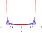
(a) $a_{0}=\cos(\pi/4)$,

$a_{1}=\cos(\pi/6)$

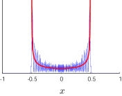
(b) $a_{0}=\cos(\pi/4)$,

$a_{1}=\cos(\pi/3)$

Figure 1: The limit density function $f(x)$ (thick line) and the probability distribution at time $t=500$ (thin line).

Proof

Our approach is due to Grimmett et al. [10]. The Fourier transform becomes

$$\ket{\hat{\Psi}_{2t}(k)}=\left(\hat{H}_{1}(k)\hat{H}_{0}(k)\right)^{t}\ket{\hat{\Psi}_{0}(k)},$$ (17)

where $\hat{H}_{\gamma}(k)=R(k)H_{\gamma}\,(\gamma=0,1)$. We assume

$$H_{\gamma}=\left[\begin{array}[]{cc}\cos\theta_{\gamma}&\sin\theta_{\gamma}\\ \sin\theta_{\gamma}&-\cos\theta_{\gamma}\end{array}\right],$$ (18)

with $\theta_{\gamma}\neq\frac{\pi n}{2}\,(n\in\mathbb{Z})$ and $\theta_{0}\neq\theta_{1}$. For the other case, the argument is nearly identical to this case, so we will omit it. The two eigenvalues $\lambda_{j}(k)\,(j=0,1)$ of $\hat{H}_{1}(k)\hat{H}_{0}(k)$ are given by

$$\lambda_{j}(k)=c_{1}c_{2}\cos 2k+s_{1}s_{2}+(-1)^{j}\,i\sqrt{1-(c_{1}c_{2}\cos 2k+s_{1}s_{2})^{2}},$$ (19)

where $c_{\gamma}=\cos\theta_{\gamma},\,s_{\gamma}=\sin\theta_{\gamma}$. The eigenvector $\ket{v_{j}(k)}$ corresponding to $\lambda_{j}(k)$ is

$$\ket{v_{j}(k)}=\left[\begin{array}[]{c}s_{1}c_{2}e^{2ik}-c_{1}s_{2}\\ \left\{-c_{1}c_{2}\sin 2k+(-1)^{j}\sqrt{1-(c_{1}c_{2}\cos 2k+s_{1}s_{2})^{2}}\right\}i\end{array}\right].$$ (20)

The Fourier transform $\ket{\hat{\Psi}_{0}(k)}$ is expressed by normalized eigenvectors $\ket{v_{j}(k)}$ as follows:

$$\ket{\hat{\Psi}_{0}(k)}=\sum_{j=0}^{1}\braket{v_{j}(k)}{\hat{\Psi}_{0}(k)}\ket{v_{j}(k)}.$$ (21)

Therefore we have

$$\ket{\hat{\Psi}_{2t}(k)} = \left(\hat{H}_{1}(k)\hat{H}_{0}(k)\right)^{t}\ket{\hat{\Psi}_{0}(k)}$$ (22)

$$= \sum_{j=0}^{1}\lambda_{j}(k)^{t}\braket{v_{j}(k)}{\hat{\Psi}_{0}(k)}\ket{v_{j}(k)}.$$

The r-th moment of $X_{2t}$ is

$$E((X_{2t})^{r}) = \sum_{x\in\mathbb{Z}}x^{r}P(X_{2t}=x)$$ (23)

$$= \int_{0}^{2\pi}\frac{dk}{2\pi}\bra{\hat{\Psi}_{2t}(k)}\left(D^{r}\ket{\hat{\Psi}_{2t}(k)}\right)$$

$$= \int_{0}^{2\pi}\sum_{j=0}^{1}(t)_{r}\lambda_{j}(k)^{-r}(D\lambda_{j}(k))^{r}\left|\braket{v_{j}(k)}{\hat{\Psi}_{0}(k)}\right|^{2}$$

$$+O(t^{r-1}),$$

where $D=i(d/dk)$ and $(t)_{r}=t(t-1)\times\cdots\times(t-r+1)$. Let $h_{j}(k)=D\lambda_{j}(k)/2\lambda_{j}(k)$. Then we obtain

$$E((X_{2t}/2t)^{r})\rightarrow\int_{\Omega_{0}}\frac{dk}{2\pi}\sum_{j=0}^{1}h^{r}_{j}(k)|\braket{v_{j}(k)}{\hat{\Psi}_{0}(k)}|^{2}\quad(\,t\rightarrow\infty).$$ (24)

Substituting $h_{j}(k)=x$, we have

$$\lim_{t\rightarrow\infty}E((X_{2t}/2t)^{r})=\int_{-|c_{\xi}|}^{|c_{\xi}|}x^{r}\,f(x)\,dx,$$ (25)

where

$$f(x)=f_{K}(x;c_{\xi})\left[1-\left\{|\alpha|^{2}-|\beta|^{2}+\frac{(\alpha\bar{\beta}+\bar{\alpha}\beta)s_{1}}{c_{1}}\right\}x\right],$$ (26)

and $|c_{\xi}|=|\cos\theta_{\xi}|=\min\left\{|\cos\theta_{0}|,|\cos\theta_{1}|\right\}$. Since $f(x)$ is the limit density function, the proof is complete. ∎

4 Special cases in time-dependent QWs

In the previous section, we have obtained the limit theorem for the two-period QW determined by two orthogonal matrices. For other two-period case and general $n$-period ($n\geq 3$) case, we think that it would be hard to get the limit theorem in a similar fashion. Here we consider two special cases in the time-dependent QWs and give the weak limit theorems.

4.1 Case 1

Let us consider the QW whose evolution is determined by the following unitary matrix:

$$U_{t}=\left[\begin{array}[]{cc}ae^{iw_{t}}&b\\ c&de^{-iw_{t}}\end{array}\right],$$ (27)

with $a,b,c,d\,\in\,\mathbb{C}$. Here $w_{t}\in\mathbb{R}$ satisfies $w_{t+1}+w_{t}=\kappa_{1}$, where $\kappa_{1}\in\mathbb{R}$ and $\mathbb{R}$ is the set of real numbers. Note that $\kappa_{1}$ does not depend on time. In this case, $w_{t}$ can be written as $w_{t}=(-1)^{t}(w_{0}-\frac{\kappa_{1}}{2})+\frac{\kappa_{1}}{2}$. Therefore the period of the QW becomes two. We should remark that $\left[\begin{array}[]{cc}a&b\\ c&d\end{array}\right](\,\equiv U\,)$ is a unitary matrix. Then we have

Theorem 4.1

$$\frac{X_{t}}{t}\,\Rightarrow\,Z_{1},$$ (28)

where $Z_{1}$ has the density function $f_{1}(x)$ as follows:

$$f_{1}(x)=f_{K}(x;a)\left\{1-\left(|\alpha|^{2}-|\beta|^{2}+\frac{a\alpha\overline{b\beta}e^{iw_{0}}+\overline{a\alpha}b\beta e^{-iw_{0}}}{|a|^{2}}\right)x\right\}.$$ (29)

Proof

The essential point of this proof is that this case results in the usual walk. First we see that $U_{t}$ can be rewritten as

$$U_{t} = \left[\begin{array}[]{cc}e^{iw_{t}/2}&0\\ 0&e^{-iw_{t}/2}\end{array}\right]\left[\begin{array}[]{cc}a&b\\ c&d\end{array}\right]\left[\begin{array}[]{cc}e^{iw_{t}/2}&0\\ 0&e^{-iw_{t}/2}\end{array}\right]$$ (36)

$$= R\left(\frac{w_{t}}{2}\right)UR\left(\frac{w_{t}}{2}\right).$$ (37)

From this, the Fourier transform $\ket{\hat{\Psi}_{t}(k)}$ can be computed in the following.

$$\ket{\hat{\Psi}_{t}(k)} = \left\{R(k)R\left(\frac{w_{t-1}}{2}\right)UR\left(\frac{w_{t-1}}{2}\right)\right\}\left\{R(k)R\left(\frac{w_{t-2}}{2}\right)UR\left(\frac{w_{t-2}}{2}\right)\right\}$$ (38)

$$\cdots\left\{R(k)R\left(\frac{w_{0}}{2}\right)UR\left(\frac{w_{0}}{2}\right)\right\}\ket{\hat{\Psi}_{0}(k)}$$

$$= R\left(-\frac{w_{t}}{2}\right)\left\{R\left(\frac{w_{t}}{2}\right)R(k)R\left(\frac{w_{t-1}}{2}\right)U\right\}$$

$$\times\left\{R\left(\frac{w_{t-1}}{2}\right)R(k)R\left(\frac{w_{t-2}}{2}\right)U\right\}$$

$$\times\cdots\times\left\{R\left(\frac{w_{1}}{2}\right)R(k)R\left(\frac{w_{0}}{2}\right)U\right\}R\left(\frac{w_{0}}{2}\right)\ket{\hat{\Psi}_{0}(k)}$$

$$= R\left(-\frac{w_{t}}{2}\right)\left\{R(k+\kappa_{1}/2)U\right\}^{t}R\left(\frac{w_{0}}{2}\right)\ket{\hat{\Psi}_{0}(k)}.$$

Therefore we have

$$\ket{\psi_{t}(x)} = \int_{0}^{2\pi}\frac{dk}{2\pi}e^{ikx}\ket{\hat{\Psi}_{t}(k)}=\int_{\kappa_{1}/2}^{2\pi+\kappa_{1}/2}\frac{dk}{2\pi}e^{i(k-\kappa_{1}/2)x}\ket{\hat{\Psi}_{t}(k-\kappa_{1}/2)}$$ (39)

$$= e^{-i\kappa_{1}x/2}R\left(-\frac{w_{t}}{2}\right)\int_{\kappa_{1}/2}^{2\pi+\kappa_{1}/2}\frac{dk}{2\pi}e^{ikx}\left(R(k)U\right)^{t}\ket{\hat{\Psi}^{R}_{0}(k)},$$

where $\ket{\hat{\Psi}^{R}_{0}(k)}=R\left(\frac{w_{0}}{2}\right)\ket{\hat{\Psi}_{0}(k-\kappa_{1}/2)}$. Then the probability distribution is

$$P(X_{t}=x)$$

$$= \left\{e^{i\kappa_{1}x/2}\left(\int_{\kappa_{1}/2}^{2\pi+\kappa_{1}/2}\frac{dk}{2\pi}e^{ikx}\left(R(k)U\right)^{t}\ket{\hat{\Psi}^{R}_{0}(k)}\right)^{\!\!\ast}R\left(\frac{w_{t}}{2}\right)\right\}$$

$$\times\left\{e^{-i\kappa_{1}x/2}R\left(-\frac{w_{t}}{2}\right)\left(\int_{\kappa_{1}/2}^{2\pi+\kappa_{1}/2}\frac{dk}{2\pi}e^{ikx}\left(R(k)U\right)^{t}\ket{\hat{\Psi}^{R}_{0}(k)}\right)\right\}$$

$$= \left|\left|\int_{\kappa_{1}/2}^{2\pi+\kappa_{1}/2}\frac{dk}{2\pi}e^{ikx}\hat{U}(k)^{t}\ket{\hat{\Psi}^{R}_{0}(k)}\right|\right|^{2},$$ (40)

where $\hat{U}(k)=R(k)U$. This implies that Case 1 can be considered as the usual QW with the initial state $\ket{\hat{\Psi}^{R}_{0}(k)}=R\left(\frac{w_{0}}{2}\right)\ket{\hat{\Psi}_{0}(k-\kappa_{1}/2)}$ and the unitary matrix $U$. Then the initial state becomes

$$\ket{\hat{\Psi}^{R}_{0}(k)}={}^{T}[e^{iw_{0}/2}\alpha,\,e^{-iw_{0}/2}\beta],$$ (41)

that is,

$$\ket{\psi_{0}(x)}=\left\{\begin{array}[]{ll}{}^{T}[e^{iw_{0}/2}\alpha,\,e^{-iw_{0}/2}\beta]&(x=0)\\[5.69054pt] {}^{T}[0,\,0]&(x\neq 0)\end{array}\right..$$ (42)

Finally, by using the result in Konno [12, 13], we can obtain the desired limit distribution of this case. ∎

4.2 Case 2

Next we consider the QW whose dynamics is defined by the following unitary matrix:

$$U_{t}=\left[\begin{array}[]{cc}a&be^{iw_{t}}\\ ce^{-iw_{t}}&d\end{array}\right].$$ (43)

Here $w_{t}\in\mathbb{R}$ satisfies $w_{t+1}=w_{t}+\kappa_{2}$, where $\kappa_{2}\in\mathbb{R}$ does not depend on $t$. In this case, $w_{t}$ can be expressed as $w_{t}=\kappa_{2}t+w_{0}$. Noting $U_{t}=R\left(\frac{w_{t}}{2}\right)UR\left(-\frac{w_{t}}{2}\right)$, we get a similar weak limit theorem as Case 1:

Theorem 4.2

$$\frac{X_{t}}{t}\,\Rightarrow\,Z_{2},$$ (44)

where $Z_{2}$ has the density function $f_{2}(x)$ as follows:

$$f_{2}(x)=f_{K}(x;a)\left\{1-\left(|\alpha|^{2}-|\beta|^{2}+\frac{a\alpha\overline{b\beta}e^{-iw_{0}}+\overline{a\alpha}b\beta e^{iw_{0}}}{|a|^{2}}\right)x\right\}.$$ (45)

If $w_{t}=2\pi t/n\,(n=1,2,\ldots)$, $\left\{U_{t}\right\}$ becomes an $n$-period sequence. In particular, when $n=2$ and $a,b,c,d\in\mathbb{R}$, $\left\{U_{t}\right\}$ is a sequence of two-period orthogonal matrices. Then Theorem 3 is equivalent to Theorem 1 (i).

5 Conclusion and Discussion

In the final section, we draw the conclusion and discuss our two-period walks. The main result of this paper (Theorem 1) implies that if $\det(H_{1}H_{0})\\ >0$ and $\min\left\{|a_{0}|,|a_{1}|\right\}=|a_{0}|$, then the limit distribution of the two-period walk is determined by $H_{0}$. On the other hand, if $\det(H_{1}H_{0})>0$ and $\min\left\{|a_{0}|,|a_{1}|\right\}=|a_{1}|$, or $\det(H_{1}H_{0})<0$, then the limit distribution is determined by both $H_{0}$ and $H_{1}$.

Here we discuss a physical meaning of our model. We should remark that the time-dependent two-period QW is equivalent to a position-dependent two-period QW if and only if the probability amplitude of the odd position in the initial state is zero. In quantum mechanics, the Kronig-Penney model, whose potential on a lattice is periodic, has been extensively investigated, see Kittel [14]. A derivation from the discrete-time QW to the continuous-time QW, which is related to the Schrödinger equation, can be obtained by Strauch [15]. Therefore, one of interesting future problems is to clarify a relation between our discrete-time two-period QW and the Kronig-Penney model.

Acknowledgment
This work was partially supported by the Grant-in-Aid for Scientific Research (C) of Japan Society for the Promotion of Science (Grant No. 21540118).

References

- [1] Ambainis, A., Bach, E., Nayak, A., Vishwanath, A., Watrous, J.: One-dimensional quantum walks. Proceedings of the 33rd Annual ACM Symposium on Theory of Computing (2001) 37–49
- [2] Shenvi, N., Kempe, J., Whaley, K.B.: Quantum random-walk search algorithm. Phys. Rev. A 67 (2003) 052307
- [3] Kendon, V.: Decoherence in quantum walks - a review. Mathematical Structures in Computer Science 17 (2007) 1169–1220
- [4] Oka, T., Konno, N., Arita, R., Aoki, H.: Breakdown of an electric-field driven system: A mapping to a quantum walk. Phys. Rev. Lett. 94 (2005) 100602
- [5] Ribeiro, P., Milman, P., Mosseri, R.: Aperiodic quantum random walks. Phys. Rev. Lett. 93 (2004) 190503
- [6] Mackay, T.D., Bartlett, S.D., Stephenson, L.T., Sanders, B.C.: Quantum walks in higher dimensions. J. Phys. A 35 (2002) 2745–2753
- [7] Konno, N.: A path integral approach for disordered quantum walks in one dimension. Fluctuation and Noise Letters 5 (2005) L529–L537
- [8] Wójcik, A., Łuczak, T., Kurzyński, P., Grudka, A., Bednarska, M.: Quasiperiodic dynamics of a quantum walk on the line. Phys. Rev. Lett. 93 (2004) 180601
- [9] Bañuls, M.C., Navarrete, C., Pérez, A., Roldán, E.: Quantum walk with a time-dependent coin. Phys. Rev. A 73 (2006) 062304
- [10] Grimmett, G., Janson, S., Scudo, P.F.: Weak limits for quantum random walks. Phys. Rev. E 69 (2004) 026119
- [11] Konno, N.: One-dimensional discrete-time quantum walks on random environments. Quantum Inf. Proc. 8 (2009) 387–399
- [12] Konno, N.: Quantum random walks in one dimension. Quantum Inf. Proc. 1 (2002) 345–354
- [13] Konno, N.: A new type of limit theorems for the one-dimensional quantum random walk. J. Math. Soc. Jpn. 57 (2005) 1179–1195
- [14] Kittel, C.: Introduction to Solid State Physics. 8 edn. Wiley (2005)
- [15] Strauch, F.W.: Connecting the discrete and continuous-time quantum walks. Phys. Rev. A 74 (2006) 030301