Improved Sparse Recovery Thresholds with Two-Step Reweighted $\ell_{1}$ Minimization

Abstract

It is well known that $\ell_{1}$ minimization can be used to recover sufficiently sparse unknown signals from compressed linear measurements. In fact, exact thresholds on the sparsity, as a function of the ratio between the system dimensions, so that with high probability almost all sparse signals can be recovered from iid Gaussian measurements, have been computed and are referred to as “weak thresholds” [4]. In this paper, we introduce a reweighted $\ell_{1}$ recovery algorithm composed of two steps: a standard $\ell_{1}$ minimization step to identify a set of entries where the signal is likely to reside, and a weighted $\ell_{1}$ minimization step where entries outside this set are penalized. For signals where the non-sparse component has iid Gaussian entries, we prove a “strict” improvement in the weak recovery threshold. Simulations suggest that the improvement can be quite impressive—over 20% in the example we consider.

I Introduction

Compressed sensing addresses the problem of recovering sparse signals from under-determined systems of linear equations [12]. In particular, if ${\bf x}$ is a $n\times 1$ real vector that is known to have at most $k$ nonzero elements where $k<n$, and ${\bf A}$ is a $m\times n$ measurement matrix with $k<m<n$, then for appropriate values of $k$, $m$ and $n$, it is possible to efficiently recover ${\bf x}$ from ${\bf y}={\bf A}{\bf x}$ [1, 2, 3, 5]. The most well recognized such algorithm is $\ell_{1}$ minimization which can be formulated as follows:

$$\min_{{\bf A}{\bf z}={\bf A}{\bf x}}\|{\bf z}\|_{1}$$ (1)

The first result that established the fundamental limits of signal recovery using $\ell_{1}$ minimization is due to Donoho and Tanner [4, 2], where it is shown that if the measurement matrix is iid Gaussian, for a given ratio of $\delta=\frac{m}{n}$, $\ell_{1}$ minimization can successfully recover every $k$-sparse signal, provided that $\mu=\frac{k}{n}$ is smaller that a certain threshold. This statement is true asymptotically as $n\rightarrow\infty$ and with high probability. This threshold guarantees the recovery of all sufficiently sparse signals and is therefore referred to as a strong threshold. It therefore does not depend on the actual distribution of the nonzero entries of the sparse signal and as such is a universal result. At this point it is not known whether there exists other polynomial-time algorithms with superior strong threshold.

Another notion introduced and computed in [4, 2] is that of a weak threshold where signal recovery is guaranteed for almost all support sets and almost all sign patterns of the sparse signal, with high probability as $n\rightarrow\infty$. The weak threshold is the one that can be observed in simulations of $\ell_{1}$ minimization and allows for signal recovery beyond the strong threshold. It is also universal in the sense that it applies to all symmetric distributions that one may draw the nonzero signal entries from. Finally, it is not known whether there exists other polynomial-time algorithms with superior weak thresholds.

In this paper we prove that a certain iterative reweighted $\ell_{1}$ algorithm indeed has better weak recovery guarantees for particular classes of sparse signals, including sparse Gaussian signals. We had previously introduced these algorithms in [11], and had proven that for a very restricted class of polynomially decaying sparse signals they outperform standard $\ell_{1}$ minimization. In this paper however, we extend this result to a much wider and more reasonable class of sparse signals. The key to our result is the fact that for these classes of signals, $\ell_{1}$ minimization has an approximate support recovery property which can be exploited via a reweighted $\ell_{1}$ algorithm, to obtain a provably superior weak threshold. In particular, we consider Gaussian sparse signals, namely sparse signals where the nonzero entries are iid Gaussian. Our analysis of Gaussian sparse signals relies on concentration bounds on the partial sum of their order statistics. Though not done here, it can be shown that for symmetric distributions with sufficiently fast decaying tails and nonzero value at the origin, similar bounds and improvements on the weak threshold can be achieved.

It is worth noting that different variations of reweighted $\ell_{1}$ algorithms have been recently introduced in the literature and, have shown experimental improvement over ordinary $\ell_{1}$ minimization [10, 7]. In [7] approximately sparse signals have been considered, where perfect recovery is never possible. However, it has been shown that the recovery noise can be reduced using an iterative scheme. In [10], a similar algorithm is suggested and is empirically shown to outperform $\ell_{1}$ minimization for exactly sparse signals with non-flat distributions. Unfortunately, [10] provides no theoretical analysis or performance guarantee. The particular reweighted $\ell_{1}$ minimization algorithm that we propose and analyze is of signiciantly less computational complexity than the earlier ones (it only solves two linear programs). Furthermore, experimental results confirm that it exhibits much better performance than previous reweighted methods. Finally, while we do rigorously establish an improvement in the weak threshold, we currently do not have tight bounds on the new weak threshold and simulation results are far better than the bounds we can provide at this time.

II Basic Definitions

A sparse signal with exactly $k$ nonzero entries is called $k$-sparse. For a vector ${\bf x}$, $\|{\bf x}\|_{1}$ denotes the $\ell_{1}$ norm. The support (set) of ${\bf x}$, denoted by $supp({\bf x})$, is the index set of its nonzero coordinates. For a vector ${\bf x}$ that is not exactly $k$-sparse, we define the $k$-support of ${\bf x}$ to be the index set of the largest $k$ entries of ${\bf x}$ in amplitude, and denote it by $supp_{k}({\bf x})$. For a subset $K$ of the entries of ${\bf x}$, ${\bf x}_{K}$ means the vector formed by those entries of ${\bf x}$ indexed in $K$. Finally, $\max|{\bf x}|$ and $\min|{\bf x}|$ mean the absolute value of the maximum and minimum entry of ${\bf x}$ in magnitude, respectively.

III Signal Model and Problem Description

We consider sparse random signals with iid Gaussian nonzero entries. In other words we assume that the unknown sparse signal is a $n\times 1$ vector ${\bf x}$ with exactly $k$ nonzero entries, where each nonzero entry is independently derived from the standard normal distribution $\mathcal{N}(0,1)$. The measurement matrix ${\bf A}$ is a $m\times n$ matrix with iid Gaussian entries with a ratio of dimensions $\delta=\frac{m}{n}$. Compressed sensing theory guarantees that if $\mu=\frac{k}{n}$ is smaller than a certain threshold, then every $k$-sparse signal can be recovered using $\ell_{1}$ minimization. The relationship between $\delta$ and the maximum threshold of $\mu$ for which such a guarantee exists is called the strong sparsity threshold, and is denoted by $\mu_{S}(\delta)$. A more practical performance guarantee is the so-called weak sparsity threshold, denoted by $\mu_{W}(\delta)$, and has the following interpretation. For a fixed value of $\delta=\frac{m}{n}$ and iid Gaussian matrix ${\bf A}$ of size $m\times n$, a random $k$-sparse vector ${\bf x}$ of size $n\times 1$ with a randomly chosen support set and a random sign pattern can be recovered from ${\bf A}{\bf x}$ using $\ell_{1}$ minimization with high probability, if $\frac{k}{n}<\mu_{W}(\delta)$. Similar recovery thresholds can be obtained by imposing more or less restrictions. For example, strong and weak thresholds for nonnegative signals have been evaluated in [6].

We assume that the support size of ${\bf x}$, namely $k$, is slightly larger than the weak threshold of $\ell_{1}$ minimization. In other words, $k=(1+\epsilon_{0})\mu_{W}(\delta)$ for some $\epsilon_{0}>0$. This means that if we use $\ell_{1}$ minimization, a randomly chosen $\mu_{W}(\delta)n$-sparse signal will be recovered perfectly with very high probability, whereas a randomly selected $k$-sparse signal will not. We would like to show that for a strictly positive $\epsilon_{0}$, the iterative reweighted $\ell_{1}$ algorithm of Section IV can indeed recover a randomly selected $k$-sparse signal with high probability, which means that it has an improved weak threshold.

IV Iterative weighted $\ell_{1}$ Algorithm

We propose the following algorithm, consisting of two $\ell_{1}$ minimization steps: a standard one and a weighted one. The input to the algorithm is the vector ${\bf y}={\bf A}{\bf x}$, where ${\bf x}$ is a $k$-sparse signal with $k=(1+\epsilon_{0})\mu_{W}(\delta)n$, and the output is an approximation ${\bf x}^{*}$ to the unknown vector ${\bf x}$. We assume that $k$, or an upper bound on it, is known. Also $\omega>1$ is a predetermined weight.

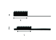
Figure 1: A pictorial example of a sparse signal and its $\ell_{1}$ minimization approximation

Algorithm 1.

1. Solve the $\ell_{1}$ minimization problem:

   $$\hat{{\bf x}}=\arg{\min{\|{\bf z}\|_{1}}}~{}~{}\text{subject to}~{}~{}{\bf A}{\bf z}={\bf A}{\bf x}.$$ (2)

2. Obtain an approximation for the support set of ${\bf x}$: find the index set $L\subset\{1,2,...,n\}$ which corresponds to the largest $k$ elements of $\hat{{\bf x}}$ in magnitude.

3. Solve the following weighted $\ell_{1}$ minimization problem and declare the solution as output:

   $${\bf x}^{*}=\arg{\min\|{\bf z}_{L}\|_{1}+\omega\|{\bf z}_{\overline{L}}\|_{1}}~{}~{}\text{subject to}~{}~{}{\bf A}{\bf z}={\bf A}{\bf x}.$$ (3)

The intuition behind the algorithm should be clear. In the first step we perform a standard $\ell_{1}$ minimization. If the sparsity of the signal is beyond the weak threshold $\mu_{W}(\delta)n$, then $\ell_{1}$ minimization is not capable of recovering the signal. However, we use the output of the $\ell_{1}$ minimization to identify an index set, $L$, which we “hope” contains most of the nonzero entries of ${\bf x}$. We finally perform a weighted $\ell_{1}$ minimization by penalizing those entries of ${\bf x}$ that are not in $L$ (ostensibly because they have a lower chance of being nonzero).

In the next sections we formally prove that the above intuition is correct and that, for certain classes of signals, Algorithm 1 has a recovery threshold beyond that of standard $\ell_{1}$ minimization. The idea of the proof is as follows. In section V, we prove that there is a large overlap between the index set $L$, found in step 2 of the algorithm, and the support set of the unknown signal ${\bf x}$ (denoted by $K$)—see Theorem 21 and Figure 1. Then in section VI, we show that the large overlap between $K$ and $L$ can result in perfect recovery of ${\bf x}$, beyond the standard weak threshold, when a weighted $\ell_{1}$ minimization is used in step 3.

V Approximate Support Recovery, Steps 1 and 2 of the Algorithm

In this Section, we carefully study the first two steps of Algorithm 1. The unknown signal ${\bf x}$ is assumed to be a Gaussian $k$-sparse vector with support set $K$, where $k=|K|=(1+\epsilon_{0})\mu_{W}(\delta)n$, for some $\epsilon_{0}>0$. By A Gaussian $k$-sparse vector, we mean one where the nonzero entries are iid Gaussian (zero mean and unit variance, say). The solution $\hat{{\bf x}}$ to the $\ell_{1}$ minimization obtained in step 1 of Algorithm 1 is in all likelihood a full vector. The set $L$, as defined in the algorithm, is in fact the $k$-support set of $\hat{{\bf x}}$. We show that for small enough $\epsilon_{0}$, the intersection of $L$ and $K$ is with high probability very large, so that $L$ can be counted as a good approximation to $K$ (Figure 1).

In order to find a decent lower bound on $|L\cap K|$, we mention three separate facts and establish a connection between them. First, we prove a general lemma that bounds $|K\cap L|$ as a function of $\|{\bf x}-\hat{{\bf x}}\|_{1}$. Then, we mention an intrinsic property of $\ell_{1}$ minimization called weak robustness that provides an upper bound on the quantity $\|{\bf x}-\hat{{\bf x}}\|_{1}$. Finally, we specifically use the Gaussianity of ${\bf x}$ to obtain Theorem 21. Let us start with a definition.

Definition 1.

For a $k$-sparse signal ${\bf x}$, we define $W({\bf x},\lambda)$ to be the size of the largest subset of nonzero entries of ${\bf x}$ that has a $\ell_{1}$ norm less than or equal to $\lambda$.

$$W({\bf x},\lambda):=\max\{|S|~{}|~{}S\subseteq supp({\bf x}),~{}\|{\bf x}_{S}\|_{1}\leq\lambda\}$$

Note that $W({\bf x},\lambda)$ is increasing in $\lambda$.

Lemma 1.

Let ${\bf x}$ be a $k$-sparse vector and $\hat{{\bf x}}$ be another vector. Also, let $K$ be the support set of ${\bf x}$ and $L$ be the $k$-support set of $\hat{{\bf x}}$. Then

$$|K\cap L|\geq k-W({\bf x},\|{\bf x}-\hat{{\bf x}}\|_{1})$$ (4)

Proof.

Let $x_{i}$ be the $i$th entry of ${\bf x}$ and ${\bf e}^{*}$ be the solution to the following minimization program

$$\min\|{\bf e}\|_{1}$$

$$\text{s.t}. \left\{\begin{array}[]{c}\max|({\bf x}+{\bf e})_{K\setminus L}|\leq\min|({\bf x}+{\bf e})_{K\cap L}|\\ \max|({\bf x}+{\bf e})_{K\setminus L}|\leq\min|({\bf x}+{\bf e})_{L\setminus K}|\end{array}\right.$$ (7)

Now since, $\hat{{\bf x}}={\bf x}+(\hat{{\bf x}}-{\bf x})$ satisfies the constraints of the minimization (7), we can write

$$\|{\bf e}^{*}\|_{1}\leq\|\hat{{\bf x}}-{\bf x}\|_{1}.$$ (8)

Let $a=\max|({\bf x}+{\bf e}^{*})_{K\setminus L}|$. Then for each $i\in K\setminus L$, using the triangular inequality we have

$$|x_{i}|-|e_{i}|\leq|x_{i}+e_{i}|\leq a$$ (9)

Therefore, by summing up the inequalities in (9) for $i\in K\setminus L$ we have

$$\|{\bf e}^{*}_{K\setminus L}\|_{1}\geq\sum_{i\in K\setminus L,|x_{i}|>a}|x_{i}|-a$$ (10)

Similarly,

$$\|{\bf e}^{*}_{L\setminus K}\|_{1}\geq a|L\setminus K|$$ (11)

But $|L\setminus K|=|K\setminus L|$ and therefore we have

$$\|{\bf e}^{*}\|_{1} \geq \sum_{i\in K\setminus L,|x_{i}|>a}(|x_{i}|-a)+a|K\setminus L|$$ (12)

$$\geq \sum_{i\in K\setminus L}|x_{i}|$$

(8) and (12) together imply that $\|{\bf x}-\hat{{\bf x}}\|_{1}\geq\|{\bf x}_{K\setminus L}\|_{1}$, which by definition means that $W({\bf x},\|{\bf x}-\hat{{\bf x}}\|_{1})\geq|K\setminus L|$.   

We now introduce the notion of weak robustness, which allows us to bound $\|{\bf x}-\hat{{\bf x}}\|_{1}$, and has the following formal definition [9].

Definition 2.

Let the set $S\subset\{1,2,\cdots,n\}$ and the subvector ${\bf x}_{S}$ be fixed. A solution $\hat{{\bf x}}$ is called weakly robust if, for some $C>1$ called the robustness factor, and all ${\bf x}_{\overline{S}}$, it holds that

$$\|({\bf x}-\hat{{\bf x}})_{S}\|_{1}\leq\frac{2C}{C-1}\|{\bf x}_{\overline{S}}\|_{1}$$ (13)

and

$$\|{\bf x}_{S}\|-\|\hat{{\bf x}}_{S}\|\leq\frac{2}{C-1}\|{\bf x}_{\overline{S}}\|_{1}$$ (14)

The weak robustness notion allows us to bound the error in $\|{\bf x}-\hat{{\bf x}}\|_{1}$ in the following way. If the matrix ${\bf A}_{S}$ , obtained by retaining only those columns of ${\bf A}$ that are indexed by $S$, has full column rank, then the quantity

$$~{}\kappa=\max_{{\bf A}{\bf w}=0,{\bf w}\neq 0}\frac{\|{\bf w}_{S}\|_{1}}{\|{\bf w}_{\overline{S}}\|_{1}}$$

must be finite, and one can write

$$\|{\bf x}-\hat{{\bf x}}\|_{1}\leq\frac{2C(1+\kappa)}{C-1}\|{\bf x}_{\overline{S}}\|_{1}$$ (15)

In [9], it has been shown that for Gaussian iid measurement matrices ${\bf A}$, $\ell_{1}$ minimization is weakly robust, i.e., there exists a robustness factor $C>1$ as a function of $\frac{|S|}{n}<\mu_{W}(\delta)$ for which (13) and (14) hold. Now let $k_{1}=(1-\epsilon_{1})\mu_{W}(\delta)n$ for some small $\epsilon_{1}>0$, and $K_{1}$ be the $k_{1}$-support set of ${\bf x}$, namely, the set of the largest $k_{1}$ entries of ${\bf x}$ in magnitude. Based on equation (15) we may write

$$\|{\bf x}-\hat{{\bf x}}\|_{1}\leq\frac{2C(1+\kappa)}{C-1}\|{\bf x}_{\overline{K_{1}}}\|_{1}$$ (16)

For a fixed value of $\delta$, $C$ in (16) is a function of $\epsilon_{1}$ and becomes arbitrarily close to $1$ as $\epsilon_{1}\rightarrow 0$. $\kappa$ is also a bounded function of $\epsilon_{1}$ and therefore we may replace it with an upper bound $\kappa^{*}$. We now have a bound on $\|{\bf x}-\hat{{\bf x}}\|_{1}$. To explore this inequality and understand its asymptotic behavior, we apply a third result, which is a certain concentration bound on the order statistics of Gaussian random variables.

Lemma 2.

Suppose $X_{1},X_{2},\cdots,X_{n}$ are $N$ iid $\mathcal{N}(0,1)$ random variables. Let $S_{N}=\sum_{i=1}^{N}|X_{i}|$ and let $S_{M}$ be the sum of the largest $M$ numbers among the $|X_{i}|$, for each $1\leq M<N$. Then for every $\epsilon>0$, as $N\rightarrow\infty$, we have

$$\mathbb{P}(|\frac{S_{N}}{N}-\sqrt{\frac{2}{\pi}}|>\epsilon)\rightarrow 0,$$ (17)

$$\mathbb{P}(|\frac{S_{M}}{S_{N}}-\exp(-\frac{\Psi^{2}(\frac{M}{2N})}{2})|>\epsilon)\rightarrow 0$$ (18)

where $\Psi(x)=Q^{-1}(x)$ with $Q(x)=\frac{1}{\sqrt{2\pi}}\int_{x}^{\infty}e^{-\frac{y^{2}}{2}}dy$.

As a direct consequence of Lemma 2 we can write:

$$\mathbb{P}(|\frac{\|{\bf x}_{\overline{K_{1}}}\|_{1}}{\|{\bf x}\|_{1}}-(1-e^{-0.5\Psi^{2}(0.5\frac{1-\epsilon_{1}}{1+\epsilon_{0}})})|>\epsilon)\rightarrow 0$$ (19)

for all $\epsilon>0$ as $n\rightarrow\infty$. Define

$$\zeta(\epsilon_{0}):=\inf_{\epsilon_{1}>0}\frac{2C(1+\kappa^{*})}{C-1}(1-e^{-0.5\Psi^{2}(0.5\frac{1-\epsilon_{1}}{1+\epsilon_{0}})})$$

Incorporating (16) into (19) we may write

$$\mathbb{P}(\frac{\|{\bf x}-\hat{{\bf x}}\|_{1}}{\|{\bf x}\|_{1}}-\zeta(\epsilon_{0})<\epsilon)\rightarrow 1$$ (20)

for all $\epsilon>0$ as $n\rightarrow\infty$. Let us summarize our conclusions so far. First, we were able to show that $|K\cap L|\geq k-W({\bf x},\|{\bf x}-\hat{{\bf x}}\|_{1})$. Weak robustness of $\ell_{1}$ minimization and Gaussianity of the signal then led us to the fact that for large $n$ with high probability $\|{\bf x}-\hat{{\bf x}}\|_{1}\leq\zeta(\epsilon_{0})\|{\bf x}\|_{1}$. These results build up the next key theorem, which is the conclusion of this section.

Theorem 1 (Support Recovery).

Let ${\bf A}$ be an iid Gaussian $m\times n$ measurement matrix with $\frac{m}{n}=\delta$. Let $k=(1+\epsilon_{0})\mu_{W}(\delta)$ and ${\bf x}$ be a $n\times 1$ random Gaussian $k$-sparse signal. Suppose that $\hat{{\bf x}}$ is the approximation to ${\bf x}$ given by the $\ell_{1}$ minimization, i.e. $\hat{{\bf x}}=argmin_{{\bf A}{\bf z}={\bf A}{\bf x}}\|{\bf z}\|_{1}$. Then, as $n\rightarrow\infty$, for all $\epsilon>0$,

$$\small\mathbb{P}(\frac{|supp({\bf x})\cap supp_{k}(\hat{{\bf x}})|}{k}-2Q(\sqrt{-2\log(1-\zeta(\epsilon_{0}))})>-\epsilon)\rightarrow 1.$$ (21)

Proof.

For each $\epsilon^{\prime}>0$ and large enough $n$, with high probability it holds that $\|{\bf x}-\hat{{\bf x}}\|_{1}<(\zeta(\epsilon_{0})+\epsilon^{\prime})\|{\bf x}\|_{1}$. Therefore, from Lemma 4 and the fact that $W({\bf x},\lambda)$ is increasing in $\lambda$, $|K\cap L|\geq k-W({\bf x},(\zeta(\epsilon_{0})+\epsilon^{\prime})\|{\bf x}\|_{1})$ with high probability. Also, an implication of Lemma 2 reveals that for any positive $\epsilon^{\prime\prime}$ and $\alpha$, $\frac{W({\bf x},\alpha\|x\|_{1})}{k}<(1-2Q(\sqrt{-2\log(1-\alpha)}))+\epsilon^{\prime\prime}$ for large enough $n$. Putting these together, we conclude that with very high probability $\frac{|K\cap L|}{k}\geq 2Q(\sqrt{-2\log(1-\zeta(\epsilon_{0})-\epsilon^{\prime})})-\epsilon^{\prime\prime}$. The desired result now follows from the continuity of the $\log(\cdot)$ and $Q(\cdot)$ functions.   

Note that if $\lim_{\epsilon_{0}\rightarrow 0}\zeta(\epsilon_{0})=0$, then Theorem 21 implies that $\frac{|K\cap L|}{k}$ becomes arbitrarily close to 1.

VI Perfect Recovery, Step 3 of the Algorithm

In Section V we showed that. if $\epsilon_{0}$ is small, the $k$-support of $\hat{{\bf x}}$, namely $L=supp_{k}(\hat{{\bf x}})$, has a significant overlap with the true support of ${\bf x}$. We even found a quantitative lower bound on the size of this overlap in Theorem 21. In step 3 of Algorithm 1, weighted $\ell_{1}$ minimization is used, where the entries in $\overline{L}$ are assigned a higher weight than those in $L$. In [8], we have been able to analyze the performance of such weighted $\ell_{1}$ minimization algorithms. The idea is that if a sparse vector ${\bf x}$ can be partitioned into two sets $L$ and $\overline{L}$, where in one set the fraction of non-zeros is much larger than in the other set, then (3) can potentially recover ${\bf x}$ with an appropriate choice of the weight $\omega>1$, even though $\ell_{1}$ minimization cannot. The following theorem can be deduced from [8].

Theorem 2.

Let $L\subset\{1,2,\cdots,n\}$ , $\omega>1$ and the fractions $f_{1},f_{2}\in[0,1]$ be given. Let $\gamma_{1}=\frac{|L|}{n}$ and $\gamma_{2}=1-\gamma_{1}$. There exists a threshold $\delta_{c}(\gamma_{1},\gamma_{2},f_{1},f_{2},\omega)$ such that with high probability, almost all random sparse vectors ${\bf x}$ with at least $f_{1}\gamma_{1}n$ nonzero entries over the set $L$, and at most $f_{2}\gamma_{2}n$ nonzero entries over the set $\overline{L}$ can be perfectly recovered using $\min_{{\bf A}{\bf z}={\bf A}{\bf x}}\|{\bf z}_{L}\|_{1}+\omega\|{\bf z}_{\overline{L}}\|_{1}$, where ${\bf A}$ is a $\delta_{c}n\times n$ matrix with iid Gaussian entries.

Furthermore, for appropriate $\omega$,

$$\mu_{W}(\delta_{c}(\gamma_{1},\gamma_{2},f_{1},f_{2},\omega))<f_{1}\gamma_{1}+f_{2}\gamma_{2},$$

i.e., standard $\ell_{1}$ minimization using a $\delta_{c}n\times n$ measurement matrix with iid Gaussian entries cannot recover such $x$.

For completeness, in Appendix A, we provide the calculation of $\delta_{c}(\gamma_{1},\gamma_{2},f_{1},f_{2},\omega)$. A software package for computing such thresholds can also be found in [13].

Theorem 3 (Perfect Recovery).

Let ${\bf A}$ be a $m\times n$ i.i.d. Gaussian matrix with $\frac{m}{n}=\delta$. If $\lim_{\epsilon_{0}\rightarrow 0}\zeta(\epsilon_{0})=0$ and $\delta_{c}(\mu_{W}(\delta),1-\mu_{W}(\delta),1,0,\omega)<\delta$, then there exist $\epsilon_{0}>0$ and $\omega>0$ so that Algorithm 1 perfectly recovers a random $(1+\epsilon_{0})\mu_{W}(\delta)$-sparse vector with i.i.d. Gaussian entries with high probability as $n$ grows to infinity.

Proof.

Leveraging on the statement of Theorem 2, in order to show that ${\bf x}$ is perfectly recovered in the last step of the algorithm, , it is sufficient to find the overlap fractions $f_{1}=\frac{|L\cap K|}{|L|}$ and $f_{2}=\frac{|\overline{L}\cap K|}{|\overline{L}|}$ for a given $\epsilon_{0}$, and show that $\delta_{c}(\frac{k}{n},1-\frac{k}{n},f_{1},f_{2},\omega)\leq\delta$. On the other hand, according to Theorem 21 as $\epsilon_{0}\rightarrow 0$, $f_{1}\rightarrow 1$ and $f_{2}\rightarrow 0$. Therefore, if $\delta_{c}(\mu_{W}(\delta),1-\mu_{W}(\delta),1,0,\omega)<\delta$, from the continuity of $\delta_{c}$ we can conclude that for a strictly positive $\epsilon_{0}$ and corresponding overlap fractions $f_{1}$ and $f_{2}$, $\delta_{c}((1+\epsilon_{0})\mu_{W}(\delta),1-(1+\epsilon_{0})\mu_{W}(\delta),f_{1},f_{2},\omega)<\delta$, which completes the proof.   

For $\delta=0.555$ it is easy to verify numerically that the conditions of Theorem 3 hold. We haven chosen $\alpha=1$ and have computed an approximate upper bound $\zeta^{*}(\epsilon_{0})$ for $\zeta(\epsilon_{0})$, using the results of [9]. This is depicted in Figure 2. As shown, when $\epsilon_{0}\rightarrow 0$, $\zeta^{*}(\epsilon_{0})$ becomes arbitrarily small too. Using this curve and the numerical $\delta_{c}$ function from Appendix A, we can show that for $\omega=10$, the value of $\epsilon_{0}=5\times 10^{-4}$ satisfies the statement of Theorem 3. This improvement is of course much smaller than what we observe in practice.

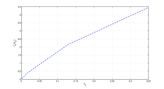
Figure 2: An approximate upper bound for $\zeta(\epsilon_{0})$ for $\delta=0.555$ .

VII Beyond Gaussians and Simulations

It is reasonable to ask if we can prove a theoretical threshold improvement for sparse signals with other distributions. The attentive reader will note that the only step where we used the Gaussianity of the signal was in the the order statistics results of Lemma 2. This result has the following interpretation. For $N$ iid random variables, the ratio $\frac{S_{M}}{S_{N}}$ can be approximated by a known function of $\frac{M}{N}$. In the Gaussian case, this function behaves as $(1-\frac{M}{N})^{2}$, as $M\rightarrow N$. For constant magnitude signals (say BPSK), the function behaves as $1-\frac{M}{N}$, for $M\rightarrow N$, which proves that the reweighted method yields no improvement. A more careful analysis, beyond the scope and space of this paper, reveals that the improvement over $\ell_{1}$ minimization depends on the behavior of $\frac{S_{M}}{S_{N}}$, as $M\rightarrow N$, which in term depends on the smallest order $n$ for which $f^{(n)}(0)\neq 0$, i.e., the smallest $n$ such that the $n$-th derivative of the distribution at the origin is nonzero.

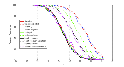
Figure 3: Empirical Recovery Percentage for $n=200$ and $\delta=0.5555$.

These are exemplified by the simulations in Figure 3. Here the signal dimension is $n=200$, and the number of measurements is $m=112$, which corresponds to a value of $\delta=0.5555$. We generated random sparse signals with iid entries coming from certain distributions; Gaussian, uniform, Rayleigh , square root of $\chi$-square with 4 degrees of freedom and, square root of $\chi$-square with 6 degrees of freedom. Solid lines represent the simulation results for ordinary $\ell_{1}$ minimization, and different colors indicate different distributions. Dashed lines are used to show the results for Algorithm 1. Note that the more derivatives that vanish at the origin, the less the improvement over $\ell_{1}$ minmimization. The Gaussian and uniform distributions are flat and nonzero at the origin and show an impressive more than 20% improvement in the weak threshold (from 45 to 55).

Appendix A Computation of $\delta_{c}$ Threshold

A. Computation of $\delta_{c}$ Threshold

The following formulas for $\delta_{c}(\gamma_{1},\gamma_{2},f_{1},f2_{,}\omega)$ are given in [8].

$$\delta_{c}= \min\{\delta~{}|~{}\psi_{com}(\tau_{1},\tau_{2})-\psi_{int}(\tau_{1},\tau_{2})-\psi_{ext}(\tau_{1},\tau_{2})<0~{}$$

$$\forall~{}0\leq\tau_{1}\leq\gamma_{1}(1-f_{1}),0\leq\tau_{2}\leq\gamma_{2}(1-f_{2}),$$

$$\tau_{1}+\tau_{2}>\delta-\gamma_{1}f_{1}-\gamma_{2}f_{2}\}$$

where $\psi_{com}$, $\psi_{int}$ and $\psi_{ext}$ are obtained as follows. Define $g(x)=\frac{2}{\sqrt{\pi}}e^{-{x^{2}}}$, $G(x)=\frac{2}{\sqrt{\pi}}\int_{0}^{x}e^{-y^{2}}dy$ and let $\varphi(.)$ and $\Phi(.)$ be the standard Gaussian pdf and cdf functions respectively.

$$\psi_{com}(\tau_{1},\tau_{2})=(\tau_{1}+\tau_{2}+\gamma_{1}(1-f_{1})H(\frac{\tau_{1}}{\gamma_{1}(1-f_{1})})$$

$$+\gamma_{2}(1-f_{2})H(\frac{\tau_{2}}{\gamma_{2}(1-f_{2})})+\gamma_{1}H(f_{1})+\gamma_{2}H(f_{2}))\log{2}$$ (22)

where $H(\cdot)$ is the Shannon entropy function. Define $c=(\tau_{1}+\gamma_{1}f_{1})+\omega^{2}(\tau_{2}+\gamma_{2}f_{2})$, $\alpha_{1}=\gamma_{1}(1-f_{1})-\tau_{1}$ and $\alpha_{2}=\gamma_{2}(1-f_{2})-\tau_{2}$. Let $x_{0}$ be the unique solution to $x$ of the equation $2c-\frac{g(x)\alpha_{1}}{xG(x)}-\frac{\omega g(\omega x)\alpha_{2}}{xG(\omega x)}=0$. Then

$$\psi_{ext}(\tau_{1},\tau_{2})=cx_{0}^{2}-\alpha_{1}\log{G(x_{0})}-\alpha_{2}\log{G(\omega x_{0})}$$ (23)

Let $b=\frac{\tau_{1}+\omega^{2}\tau_{2}}{\tau_{1}+\tau_{2}}$, $\Omega^{\prime}=\gamma_{1}f_{1}+\omega^{2}\gamma_{2}f_{2}$ and $Q(s)=\frac{\tau_{1}\varphi(s)}{(\tau_{1}+\tau_{2})\Phi(s)}+\frac{\omega\tau_{2}\varphi(\omega s)}{(\tau_{1}+\tau_{2})\Phi(\omega s)}$. Define the function $\hat{M}(s)=-\frac{s}{Q(s)}$ and solve for $s$ in $\hat{M}(s)=\frac{\tau_{1}+\tau_{2}}{(\tau_{1}+\tau_{2})b+\Omega^{\prime}}$. Let the unique solution be $s^{*}$ and set $y=s^{*}(b-\frac{1}{\hat{M}(s^{*})})$. Compute the rate function $\Lambda^{*}(y)=sy-\frac{\tau_{1}}{\tau_{1}+\tau_{2}}\Lambda_{1}(s)-\frac{\tau_{2}}{\tau_{1}+\tau_{2}}\Lambda_{1}(\omega s)$ at the point $s=s^{*}$, where $\Lambda_{1}(s)=\frac{s^{2}}{2}+\log(2\Phi(s))$. The internal angle exponent is then given by:

$$\psi_{int}(\tau_{1},\tau_{2})=(\Lambda^{*}(y)+\frac{\tau_{1}+\tau_{2}}{2\Omega^{\prime}}y^{2}+\log 2)(\tau_{1}+\tau_{2})$$ (24)

References

- [1] D. Donoho,“ Compressed sensing”, IEEE Trans. on Information Theory, 52(4), pp. 1289 - 1306, April 2006)
- [2] D. Donoho, “High-Dimensional Centrally Symmetric Polytopes with Neighborliness Proportional to Dimension ”, Discrete and Computational Geometry , 102(27), pp. 617-652, 2006, Springer .
- [3] E. Candés and T. Tao, “Decoding by linear programming”, IEEE Trans. on Information Theory, 51(12), pp. 4203 - 4215, December 2005.
- [4] D. Donoho and J. Tanner, “Thresholds for the Recovery of Sparse Solutions via L1 Minimization”, Proceedings of the Conference on Information Sciences and Systems, March 2006.
- [5] R. G. Baraniuk and M. B. Wakin “Random Projections of Smooth Manifolds ”, Journal of Foundations of Computational Mathematics, Volume 9, No.1, Feb. 2009,
- [6] D. Donoho and J. Tanner, “Sparse nonnegative solutions of underdetermined linear equations by linear programming” Proc. National Academy of Sciences, 102(27), pp.9446-9451, 2005.
- [7] D. Needell, “Noisy signal recovery via iterative reweighted L1-minimization” Proc. Asilomar Conf. on Signals, Systems, and Computers, Pacific Grove, CA Nov. 2009.
- [8] A. Khajehnejad, W. Xu, A. Avestimehr, Babak Hassibi, “Weighted minimization for Sparse Recovery with Prior Information”, accepted to the International Symposium on Information Theory 2009, available online http://arxiv.org/abs/0901.2912. Complete jounrnal manuscript to be submitted.
- [9] W. Xu and B. Hassibi, “On Sharp Performance Bounds for Robust Sparse Signal Recoveries”, accepted to the International Symposium on Information Theory 2009.
- [10] E. J. Candés, M. B. Wakin, and S. Boyd, “Enhancing Sparsity by Reweighted l1 Minimization”, Journal of Fourier Analysis and Applications, 14(5), pp. 877-905, special issue on sparsity, December 2008.
- [11] B. Hassibi, A. Khajehnejad, W. Xu, S. Avestimehr, ”Breaking the Recovery Thresholds with Reweighted Optimization,”, in proceedings of Allerton 2009.
- [12] Compressive sesing online resources at Rice university, http://www.dsp.ece.rice.edu/cs
- [13] http://www.its.caltech.edu/amin/weighted_l1_codes/