Searching for gravitational waves from known pulsars using the ${\mathcal{F}}$ and ${\mathcal{G}}$ statistics

Abstract

In searches for gravitational waves emitted by known isolated pulsars in data collected by a detector one can assume that the frequency of the wave, its spindown parameters, and the position of the source in the sky are known, so the almost monochromatic gravitational-wave signal we are looking for depends on at most four parameters: overall amplitude, initial phase, polarization angle, and inclination angle of the pulsar’s rotation axis with respect to the line of sight. We derive two statistics by means of which one can test whether data contains such gravitational-wave signal: the ${\mathcal{G}}$-statistic for signals which depend on only two unknown parameters (overall amplitude and initial phase), and the ${\mathcal{F}}$-statistic for signals depending on all four parameters. We study, by means of the Fisher matrix, the theoretical accuracy of the maximum-likelihood estimators of the signal’s parameters and we present the results of the Monte Carlo simulations we performed to test the accuracy of these estimators.

I Introduction

We study the detection of almost monochromatic gravitational waves emitted by known single pulsars in data collected by a detector. Several such searches were already performed with data collected by the LIGO and GEO600 detectors LSC04 ; LSC05 ; LSC07 ; LSC08 ; LSC10 . We thus assume that the frequency of the wave (together with its time derivatives, i.e. the spindown parameters) and the position of the source in the sky are known. The gravitational-wave signal we are looking for depends on at most four (often called amplitude) parameters: overall amplitude, initial phase, polarization angle, and inclination angle (of the pulsar’s rotation axis with respect to the line of sight).

In Sec. 2 we introduce three statistics by means of which one can test whether data contains a gravitational-wave signal: the $\mathcal{H}$-statistic for completely known signals, the ${\mathcal{G}}$-statistic for signals which depend on only two unknown parameters (overall amplitude and initial phase), and the ${\mathcal{F}}$-statistic suitable for signals depending on all four amplitude parameters. Both statistics ${\mathcal{G}}$ and ${\mathcal{F}}$ are derived from the maximum likelihood (ML) principle, and the statistic ${\mathcal{G}}$ is independently obtained using Bayesian approach and the composite hypothesis testing. In Sec. 3 we study, by means of the Fisher matrix, the theoretical accuracy of the ML estimators of the signal’s parameters and in Sec. 4 we present the results of the Monte Carlo simulations we performed to test the accuracy of the ML estimators.

II Using the ${\mathcal{F}}$ and ${\mathcal{G}}$ statistics to perform targeted searches for gravitational waves from pulsars

In the case when the signal $s(t)$ we are looking for is completely known, the test that maximizes probability of detection subject to a certain false alarm probability is the likelihood-ratio test, i.e. we accept the hypothesis that the signal is present in detector’s data $x$ if

$$\Lambda(x):=\frac{p_{1}(x)}{p_{0}(x)}\geq\lambda_{0},$$ (1)

where the likelihood function $\Lambda(x)$ is the ratio of probability densities $p_{1}(x)$ and $p_{0}(x)$ of the data $x$ when the signal is respectively present or absent. The parameter $\lambda_{0}$ is a threshold calculated from a chosen false alarm probability. Assuming stationary and additive Gaussian noise with one-sided spectral density constant (and equal to $S_{0}$) over the bandwidth of the signal, the $\log$ likelihood function is approximately given by JKS98

$$\ln\Lambda[x(t)]\cong 2\frac{T_{\text{o}}}{S_{0}}\left({\left\langle x(t)s(t)\right\rangle}-\frac{1}{2}{\left\langle s(t)^{2}\right\rangle}\right),$$ (2)

where $T_{\text{o}}$ is the observation time and the time-averaging operator ${\left\langle\cdot\right\rangle}$ is defined as

$${\left\langle g\right\rangle}:=\frac{1}{T_{\text{o}}}\int^{T_{\text{o}}}_{0}g(t)\,\mathrm{d}t.$$ (3)

Equation (2) implies that the likelihood-ratio test (1) can be replaced by the test

$${\mathcal{H}}[x(t)]:={\left\langle x(t)s(t)\right\rangle}\geq{\mathcal{H}}_{0},$$ (4)

where the optimal statistic ${\mathcal{H}}$ in this case is the matched filter and ${\mathcal{H}}_{0}$ is the threshold for detection.

Suppose now that the signal $s(t;\boldsymbol{\theta})$ depends on a set of unknown parameters $\boldsymbol{\theta}$, then a suitable test can be obtained using a Bayesian approach and composite hypothesis testing. The composite hypothesis in this case is the hypothesis that when a signal is present it can assume any values of the parameters. Assuming that the cost functions are independent of the values of the parameters, we obtain the following Bayesian decision rule to choose the hypothesis that the signal is present (see e.g. W71 , Chapter 5.9):

$$\frac{1}{p_{0}(x)}\,{\int_{\Theta}}p_{1}(x;\boldsymbol{\theta})\pi(\boldsymbol{\theta})\,\mathrm{d}\boldsymbol{\theta}\geq\gamma_{0},$$ (5)

where $\Theta$ is the parameter space on which $\boldsymbol{\theta}$ is defined and $\pi(\boldsymbol{\theta})$ is the joint a priori distribution of $\boldsymbol{\theta}$. The expression on the left hand side of Eq. (5) is know as the Bayes factor and it is the ratio between the posterior probability distribution on the signal parameters marginalized over the parameters themselves (this is the signal model Bayesian evidence) and the noise model which has no defining parameters (this is the noise model Bayesian evidence).

As a template for the response of an interferometric detector to the gravitational-wave signal from a rotating neutron star we use the model derived in JKS98 . This template depends on the set of following parameters: $\boldsymbol{\theta}=(h_{0},\phi_{0},\psi,\iota,\mathbf{f},\delta,\alpha)$, where $h_{0}$ is the dimensionless amplitude, $\phi_{0}$ is an initial phase, $\psi$ is the polarization angle, $\iota$ is the inclination angle, angles $\delta$ (declination) and $\alpha$ (right ascension) are equatorial coordinates determining the position of the source in the sky, and the ‘frequency vector’ $\mathbf{f}:=(f_{0},f_{1},f_{2},\dots)$ collects the frequency $f_{0}$ and the spindown parameters of the signal. In the case of pulsars known from radio observations we in general know the subset $\boldsymbol{\xi}=(\mathbf{f},\delta,\alpha)$ of the parameters $\boldsymbol{\theta}$.

Sometimes, like in the case of the Vela pulsar, we also know from X-ray observations the values of the angles $\psi$ and $\iota$ (see NR04 ; NR08 for observational results). We then have only two unknown parameters: $h_{0}$ and $\phi_{0}$. The response $s(t)$ of the detector to the gravitational wave we can write in this case in the following form JKS98 :

$$s(t)=h_{0}\cos\phi_{0}\,h_{c}(t)+h_{0}\sin\phi_{0}\,h_{s}(t),$$ (6)

where $h_{c}$ and $h_{s}$ are known functions of time,

$$\begin{array}[]{l}h_{c}(t):=A_{+}\big{(}\cos 2\psi\,h_{1}(t)+\sin 2\psi\,h_{2}(t)\big{)}-A_{\times}\big{(}\sin 2\psi\,h_{3}(t)-\cos 2\psi\,h_{4}(t)\big{)},\\[4.30554pt] h_{s}(t):=-A_{\times}\big{(}\sin 2\psi\,h_{1}(t)-\cos 2\psi\,h_{2}(t)\big{)}-A_{+}\big{(}\cos 2\psi\,h_{3}(t)+\sin 2\psi\,h_{4}(t)\big{)}.\end{array}$$ (7)

Here the constants $A_{+}$ and $A_{\times}$ are

$$A_{+}:=\frac{1}{2}(1+\cos^{2}\iota),\quad A_{\times}:=\cos\iota,$$ (8)

and the four functions of time $h_{k}$ $(k=1,\ldots,4)$ depend only on parameters $\boldsymbol{\xi}$ and are defined as follows

$$\begin{array}[]{ll}h_{1}(t;\boldsymbol{\xi}):=a(t;\delta,\alpha)\cos\phi(t;\mathbf{f},\delta,\alpha),&h_{2}(t;\boldsymbol{\xi}):=b(t;\delta,\alpha)\cos\phi(t;\mathbf{f},\delta,\alpha),\\[4.30554pt] h_{3}(t;\boldsymbol{\xi}):=a(t;\delta,\alpha)\sin\phi(t;\mathbf{f},\delta,\alpha),&h_{4}(t;\boldsymbol{\xi}):=b(t;\delta,\alpha)\sin\phi(t;\mathbf{f},\delta,\alpha),\end{array}$$ (9)

where $a$, $b$ are the amplitude modulation functions and $\phi$ is the phase modulation function. Their explicit forms are given in JKS98 .

Let us calculate the likelihood function for the signal (6). Observing that the amplitude modulation functions $a$ and $b$ vary much more slowly than the phase $\phi$ of the signal and assuming that the observation time is much longer than the period of the signal we approximately have JKS98

$$\begin{array}[]{l}{\left\langle h_{1}\,h_{3}\right\rangle}\cong{\left\langle h_{1}\,h_{4}\right\rangle}\cong{\left\langle h_{2}\,h_{3}\right\rangle}\cong{\left\langle h_{2}\,h_{4}\right\rangle}\cong 0,\\[4.30554pt] {\left\langle h_{1}\,h_{1}\right\rangle}\cong{\left\langle h_{3}\,h_{3}\right\rangle}\cong\frac{1}{2}A,\quad{\left\langle h_{2}\,h_{2}\right\rangle}\cong{\left\langle h_{4}\,h_{4}\right\rangle}\cong\frac{1}{2}B,\quad{\left\langle h_{1}\,h_{2}\right\rangle}\cong{\left\langle h_{3}\,h_{4}\right\rangle}\cong\frac{1}{2}C,\end{array}$$ (10)

where we have introduced the time averages

$$A:={\left\langle a^{2}\right\rangle},\quad B:={\left\langle b^{2}\right\rangle},\quad C:={\left\langle ab\right\rangle}.$$ (11)

As a consequence of the above approximations we have the following approximate expressions for the time averaged products of the functions $h_{c}$ and $h_{s}$,

$${\left\langle h_{c}^{2}\right\rangle}\cong{\left\langle h_{s}^{2}\right\rangle}\cong N,\quad{\left\langle h_{c}h_{s}\right\rangle}\cong 0,$$ (12)

where $N$ is a constant defined as

$$N :=\frac{1}{2}\Big{(}A(A_{+}^{2}\cos^{2}2\psi+A_{\times}^{2}\sin^{2}2\psi)+B(A_{+}^{2}\sin^{2}2\psi+A_{\times}^{2}\cos^{2}2\psi)$$

$$\qquad+C(A_{+}^{2}-A_{\times}^{2})\sin 4\psi\Big{)}.$$ (13)

With the above approximations the likelihood function $\Lambda$ for the signal (6) can be written as

$$\ln\Lambda[x(t);\phi_{0},h_{0}]\cong 2\frac{T_{\text{o}}}{S_{0}}\left(h_{0}\cos\phi_{0}{\left\langle x(t)h_{c}(t)\right\rangle}+h_{0}\sin\phi_{0}{\left\langle x(t)h_{s}(t)\right\rangle}-\frac{1}{2}h_{0}^{2}N\right).$$ (14)

Let us also note that the optimal signal-to-noise ratio (SNR) $\rho$ for the signal (6) (see JKS98 for definition) can be approximately computed as

$$\rho\cong\sqrt{\frac{2T_{\text{o}}}{S_{0}}{\left\langle s(t)^{2}\right\rangle}}\cong\sqrt{\frac{2T_{\text{o}}N}{S_{0}}}h_{0}.$$ (15)

It is natural to assume that the prior probability density of the phase parameter $\phi_{0}$ is uniform over the interval $[0,2\pi)$ and that it is independent of the distribution of the amplitude parameter $h_{0}$, i.e.

$$\pi(\phi_{0})=\frac{1}{2\pi},\quad\phi\in[0,2\pi).$$ (16)

With the above assumptions the integral $\int_{0}^{2\pi}p_{1}(x;\phi_{0},h_{0})\pi(\phi_{0})\mathrm{d}\phi_{0}$ can be explicitly calculated (see W71 , Chapter 7.2) and we obtain the following decision criterion

$$\exp\bigg{(}-\frac{h_{0}^{2}NT_{\text{o}}}{S_{0}}\bigg{)}\,I_{0}\bigg{(}2h_{0}\sqrt{\frac{T_{\text{o}}N}{S_{0}}{\mathcal{G}}[x(t)]}\bigg{)}\geq\gamma_{0},$$ (17)

where $I_{0}$ is the modified Bessel function of zero order and the statistic ${\mathcal{G}}$ is defined as

$${\mathcal{G}}[x(t)]:=\frac{T_{\text{o}}}{NS_{0}}\Big{(}{\left\langle x(t)h_{c}(t)\right\rangle}^{2}+{\left\langle x(t)h_{s}(t)\right\rangle}^{2}\Big{)}.$$ (18)

The function on the left-hand side of Eq. (17) is a monotonically increasing function of ${\mathcal{G}}$ and it can be maximized if ${\mathcal{G}}$ is maximized independently of the value of $h_{0}$. Thus the test

$${\mathcal{G}}[x(t)]\geq{\mathcal{G}}_{0},$$ (19)

provides a uniformly most powerful test with respect to the amplitude $h_{0}$.

When we have no a priori information about the parameters a standard method is the maximum likelihood (ML) detection which consists of maximizing the likelihood function $\Lambda[x(t);\boldsymbol{\theta}]$ with respect to the parameters of the signal. If the maximum of $\Lambda$ exceeds a certain threshold we say that the signal is detected. The values of the parameters that maximize $\Lambda$ are said to be the ML estimators of the parameters of the signal. For the case of signal (6) it is convenient to introduce new parameters

$$A_{c}:=h_{0}\cos\phi_{0},\quad A_{s}:=h_{0}\sin\phi_{0}.$$ (20)

Then one can find the ML estimators of the amplitudes $A_{c}$ and $A_{s}$ in a closed analytic form,

$$\hat{A}_{c}\cong\frac{{\left\langle xh_{c}\right\rangle}}{N},\quad\hat{A}_{s}\cong\frac{{\left\langle xh_{s}\right\rangle}}{N}.$$ (21)

It is easy to find that the estimators $\hat{A}_{c}$ and $\hat{A}_{s}$ are unbiased and also that they are of minimum variance, i.e. their variances attain the lower Cramér-Rao bound determined by the Fisher matrix. The variances of both estimators are the same and equal to $1/N$. Substituting the estimators $\hat{A}_{c}$ and $\hat{A}_{s}$ for the parameters $A_{c}$ and $A_{s}$ in the likelihood function one obtains a reduced likelihood function. This reduced likelihood function is precisely equal to the ${\mathcal{G}}$-statistic given by Eq. (18), i.e. ${\mathcal{G}}[x(t)]=\ln\Lambda[x(t);\hat{A}_{c},\hat{A}_{s}]$. The formula for the ${\mathcal{G}}$-statistic obtained without usage of the simplifying assumptions (10) is given in Appendix A.

When the all four parameters $(h_{0},\phi_{0},\psi,\iota)$ are unknown one can introduce new parameters $A_{k}$ ($k=1,\ldots,4$) that are functions of $(h_{0},\phi_{0},\psi,\iota)$ such that the response $s(t)$ takes the form

$$s(t)=A_{1}\,h_{1}(t)+A_{2}\,h_{2}(t)+A_{3}\,h_{3}(t)+A_{4}\,h_{4}(t),$$ (22)

where the functions $h_{k}$ are given by Eqs. (9) and the parameters $A_{k}$ read

$$\begin{array}[]{l}A_{1}:=h_{0+}\cos 2\psi\cos\phi_{0}-h_{0\times}\sin 2\psi\sin\phi_{0},\\[4.30554pt] A_{2}:=h_{0+}\sin 2\psi\cos\phi_{0}+h_{0\times}\cos 2\psi\sin\phi_{0},\\[4.30554pt] A_{3}:=-h_{0+}\cos 2\psi\sin\phi_{0}-h_{0\times}\sin 2\psi\cos\phi_{0},\\[4.30554pt] A_{4}:=-h_{0+}\sin 2\psi\sin\phi_{0}+h_{0\times}\cos 2\psi\cos\phi_{0};\end{array}$$ (23)

here $h_{0+}:=h_{0}\,A_{+}$ and $h_{0\times}:=h_{0}\,A_{\times}$ [see Eq. (8)]. The ML estimators of $A_{k}$ can again be obtained in an explicit analytic form and the reduced likelihood function is the ${\mathcal{F}}$-statistic given by (see JKS98 for details)

$${\mathcal{F}}[x(t)]:=\ln\Lambda[x(t);\hat{A}_{1},\ldots,\hat{A}_{4}]\cong \,\frac{2T_{\text{o}}}{S_{0}D}\Big{(}B\,({\left\langle xh_{1}\right\rangle}^{2}+{\left\langle xh_{3}\right\rangle}^{2})+A\,({\left\langle xh_{2}\right\rangle}^{2}+{\left\langle xh_{4}\right\rangle}^{2})$$

$$\qquad\quad-2C\,({\left\langle xh_{1}\right\rangle}{\left\langle xh_{2}\right\rangle}+{\left\langle xh_{3}\right\rangle}{\left\langle xh_{4}\right\rangle})\Big{)},$$ (24)

where $D:=AB-C^{2}$. The test

$${\mathcal{F}}[x(t)]\geq{\mathcal{F}}_{0}$$ (25)

is not a uniformly most powerful test with respect to unknown parameters $(h_{0},\phi_{0},\psi,\iota)$. It was recently shown that uniform a priori distributions of $(h_{0},\phi_{0},\psi,\cos\iota)$ lead to a statistic that can be more powerful than ${\mathcal{F}}$ PK09 .

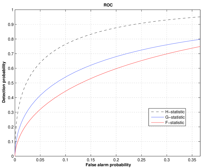
In Fig. 1 we have plotted the receiver operating characteristics (ROC) for the three statistics ${\mathcal{H}}$, ${\mathcal{G}}$, and ${\mathcal{F}}$ considered in the present section.

Figure 1: Receiver operating characteristic (ROC) for the statistics ${\mathcal{H}}$, ${\mathcal{G}}$, and ${\mathcal{F}}$ for the optimal signal-to-noise ratio $\rho=2$.

III The Fisher matrix

Using the Fisher matrix we can assess the accuracy of the parameter estimators. We have two theorems that can loosely be stated as follows.

Theorem 1 (Cramèr-Rao bound)

The diagonal elements of the inverse of the Fisher matrix are lower bounds on the variances of unbiased estimators of the parameters.

Theorem 2

Asymptotically (i.e. when the SNR tends to infinity) the ML estimators are unbiased and their covariance matrix is equal to the inverse of the Fisher matrix.

For an almost monochromatic signal $s=s(t;\boldsymbol{\theta})$, which depends on the parameters $\boldsymbol{\theta}=(\theta_{1},\ldots,\boldsymbol{\theta}_{m})$, the elements of the Fisher matrix $\Gamma$ can be approximately calculated from the formula

$$\Gamma_{{\theta_{i}}{\theta_{j}}}\cong\frac{2T_{\text{o}}}{S_{0}}{\left\langle\frac{\partial s}{\partial\theta_{i}}\frac{\partial s}{\partial\theta_{j}}\right\rangle},\quad i,j=1,\ldots,m.$$ (26)

In the case when only the parameters $h_{0}$ and $\phi_{0}$ are unknown (${\mathcal{G}}$-statistic search), the Fisher matrix can be computed easily from Eqs. (6) and (26). It is diagonal and the standard deviations of the parameters defined as the square roots of the diagonal elements of the inverse of the Fisher matrix read:

$$\frac{\sigma_{h_{0}}}{h_{0}}=\frac{1}{\rho},\quad\sigma_{\phi_{0}}=\frac{1}{\rho},$$ (27)

where $\rho$ is the optimal SNR [given in Eq. (15)].

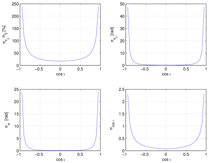
Figure 2: Dependence of standard deviations (calculated from the Fisher matrix) of the parameters $h_{0}$, $\phi_{0}$, $\psi$, and $\cos\iota$ on the cosine of the inclination angle $\iota$. We have taken $\phi_{0}=4.03$ and $\psi=-0.22$ (values of other parameters needed to perform the computation of the Fisher matrix are listed in the text of Sec. 3).

When all the four amplitude parameters $h_{0}$, $\phi_{0}$, $\psi$, and $\iota$ are unknown (${\mathcal{F}}$-statistic search), the Fisher matrix can be computed by means of formulas given in Appendix B. In this case it is not diagonal, indicating that the amplitude parameters are correlated. The quantities $\sigma_{h_{0}}/h_{0}$, $\sigma_{\phi_{0}}$, $\sigma_{\psi}$, $\sigma_{\iota}$ (where the standard deviations again are defined as square roots of diagonal elements of the inverse of the Fisher matrix) have rather complicated analytical form but they possess a number of simple properties. They are inversely proportional to the overall amplitude $h_{0}$, independent on the initial phase $\phi_{0}$, and very weakly dependent on $\psi$, however there is a strong dependence on $\iota$.

In Fig. 2 we have shown the dependence of the standard deviations on the cosine of the inclination angle $\iota$. The time averages from Eqs. (11) (needed to compute the Fisher matrix) were computed here for the location of the Virgo detector Virgo08 and for a randomly chosen position of the source in the sky. We have also taken $h_{0}=6.0948\times 10^{-2}$, $T_{\text{o}}=441610$ s, and $S_{0}=2$ Hz^-1, which corresponds to the SNR $\rho\cong 28.64\sqrt{2N}$ [see Eq. (15)]. The same time averages and the values of $T_{\text{o}}$, $h_{0}$, $S_{0}$ were used in the Monte Carlo simulations described in Sec. 4. We see in Fig. 2 that the standard deviations become singular when $\cos\iota=\pm 1$. This singularity originates from the degeneracy of the amplitude parameters for $\cos\iota=\pm 1$. In this case the amplitude parameters from Eqs. (23) become

$$A_{1}=h_{0}\cos(2\psi\pm\phi_{0}),\quad A_{2}=h_{0}\sin(2\psi\pm\phi_{0}),\quad A_{3}=\mp A_{2},\quad A_{4}=\pm A_{1}.$$ (28)

Thus only two of them are independent. Therefore the determinant of the 4-dimensional Fisher matrix is equal to zero at $\cos\iota=\pm 1$ and consequently its inverse does not exist in this case.

IV Monte Carlo simulations

We have performed two Monte Carlo simulations in order to test the performance of the ML estimators. We have compared the simulated standard deviations of the estimators with the ones obtained from the Fisher matrix. In particular we have investigated the behavior of the ML estimators near the Fisher matrix singularity at $\cos\iota=\pm 1$. In each simulation run we have generated the signal using Eq. (22), we have added it to a white Gaussian noise, and we have estimated the amplitude parameters using the ${\mathcal{F}}$-statistic. Each simulation run was repeated 1000 times for different realizations of the noise.

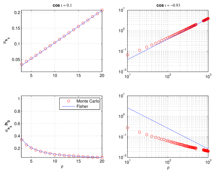
Figure 3: Mean and normalized standard deviation of the ML estimator of the amplitude $h_{0}$ as a function of the SNR. The top two panels are the means of the estimator for the two values of $\cos\iota$. The continuous line is the true value and the circles are results of the simulation for 1000 realizations of the noise. The bottom two panels are the standard deviations. The continuous line is obtained form the Fisher matrix whereas the circles are results of the simulation. We have taken $\phi_{0}=4.03$ and $\psi=-0.22$.

In the first simulation we have investigated the bias and the standard deviation of the ML estimator of the amplitude parameter $h_{0}$ as functions of the SNR for the two cases: $\cos\iota=0.1$ and $\cos\iota=-0.93$. The results are presented in Fig. 3. For the first case the ML estimator is nearly unbiased and its standard deviation is close to the one predicted by the Fisher matrix even for low SNRs. In the second case the simulation shows considerable bias of the estimator and its standard deviation lower than the one predicted by the Fisher matrix. However, Theorem 2 is satisfied in the second case. For $\cos\iota$ close to $\pm 1$ we have to go to SNR $\sim 1000$ in order for the ML estimator to be unbiased and its standard deviation close to the one given by the Fisher matrix.

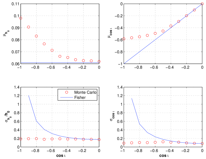
Figure 4: Means and normalized standard deviations of the ML estimators of $h_{0}$ and $\cos\iota$ as functions of $\cos\iota$. The top two panels are the means of the estimators. The continuous lines are the true values and the circles are results of the simulation for 1000 realizations of the noise. The bottom two panels are the standard deviations. The continuous lines are obtained form the Fisher matrix whereas the circles are results of the simulation. We have assumed $\phi_{0}=4.03$, $\psi=-0.22$, and $\rho=15.6$. Plots for $0\leq\cos\iota\leq+1$ (not shown here) are mirror images of the plots for $-1\leq\cos\iota\leq 0$.

In the second simulation, illustrated in Fig. 4, we have investigated the bias and the standard deviation of the ML estimators of the amplitude parameters $h_{0}$ and $\cos\iota$ as functions of $\cos\iota$ for the fixed SNR $\rho=15.6$. We find that for $|\cos\iota|<0.5$ the biases are less than 10% and the Fisher matrix overestimates the standard deviations also by less than 10%. We see that over the whole range of $\cos\iota$ the standard deviations of the parameters are roughly constant whereas the biases increases as the $|\cos\iota|$ increases. At $\cos\iota\pm 1$ the amplitude $h_{0}$ is overestimated by almost a factor of 2.

One reason why Theorem 1 does not apply here is that it holds for unbiased estimators. Also a more precise statement of Theorem 1 (see e.g. Theorem 8 in JKbook ) requires that the Fisher matrix $\Gamma$ is positive definite for all values of parameters. This last assumption is clearly not satisfied here as $\det\Gamma=0$ for $\cos\iota=\pm 1$.

Appendix A The general form of the ${\mathcal{G}}$-statistic

It is not difficult to obtain the ${\mathcal{G}}$-statistic without simplifying assumptions (10). The estimators of the amplitude parameters $A_{c}$ and $A_{s}$ are then given by

$$\hat{A}_{c}=\frac{{\left\langle h_{s}^{2}\right\rangle}{\left\langle xh_{c}\right\rangle}-{\left\langle h_{c}h_{s}\right\rangle}{\left\langle xh_{s}\right\rangle}}{{\left\langle h_{c}^{2}\right\rangle}{\left\langle h_{s}^{2}\right\rangle}-{\left\langle h_{c}h_{s}\right\rangle}^{2}},\quad\hat{A}_{s}=\frac{{\left\langle h_{c}^{2}\right\rangle}{\left\langle xh_{s}\right\rangle}-{\left\langle h_{c}h_{s}\right\rangle}{\left\langle xh_{c}\right\rangle}}{{\left\langle h_{c}^{2}\right\rangle}{\left\langle h_{s}^{2}\right\rangle}-{\left\langle h_{c}h_{s}\right\rangle}^{2}},$$ (29)

and the general form of the ${\mathcal{G}}$-statistic reads

$${\mathcal{G}}[x(t)]\cong\frac{T_{\text{o}}}{S_{0}}\left(\frac{{\left\langle h_{s}^{2}\right\rangle}{\left\langle xh_{c}\right\rangle}^{2}-2{\left\langle h_{c}h_{s}\right\rangle}{\left\langle xh_{c}\right\rangle}{\left\langle xh_{s}\right\rangle}+{\left\langle h_{c}^{2}\right\rangle}{\left\langle xh_{s}\right\rangle}^{2}}{{\left\langle h_{c}^{2}\right\rangle}{\left\langle h_{s}^{2}\right\rangle}-{\left\langle h_{c}h_{s}\right\rangle}^{2}}\right).$$ (30)

Appendix B Fisher matrix for amplitude parameters

Let us consider the gravitational-wave signal $s$ of the form

$$s(t;\mathbf{A})=\sum^{4}_{k=1}A_{k}\,h_{k}(t),$$ (31)

where the vector $\mathbf{A}$ collects the amplitude parameters, $\mathbf{A}:=(A_{1},A_{2},A_{3},A_{4})$, and the known functions $h_{k}$ ($k=1,\dots,4$) are given in Eqs. (9). We further assume, as in Sec. 2, that the noise spectral density is constant (and equal to $S_{0}$) over the bandwidth of the signal and that the approximations (10) are valid. Then the Fisher matrix for the signal’s parameters $\mathbf{A}$ reads

$$\Gamma(\mathbf{A})\cong\frac{T_{\text{o}}}{S_{0}}\begin{pmatrix}{\left\langle a^{2}\right\rangle}&{\left\langle ab\right\rangle}&0&0\\[4.30554pt] {\left\langle ab\right\rangle}&{\left\langle b^{2}\right\rangle}&0&0\\[4.30554pt] 0&0&{\left\langle a^{2}\right\rangle}&{\left\langle ab\right\rangle}\\[4.30554pt] 0&0&{\left\langle ab\right\rangle}&{\left\langle b^{2}\right\rangle}\end{pmatrix},$$ (32)

and its inverse is qual to

$$\Gamma(\mathbf{A})^{-1}\cong\frac{S_{0}}{T_{\text{o}}\big{(}{\left\langle a^{2}\right\rangle}{\left\langle b^{2}\right\rangle}-{\left\langle ab\right\rangle}^{2}\big{)}}\begin{pmatrix}{\left\langle b^{2}\right\rangle}&-{\left\langle ab\right\rangle}&0&0\\[4.30554pt] -{\left\langle ab\right\rangle}&{\left\langle a^{2}\right\rangle}&0&0\\[4.30554pt] 0&0&{\left\langle b^{2}\right\rangle}&-{\left\langle ab\right\rangle}\\[4.30554pt] 0&0&-{\left\langle ab\right\rangle}&{\left\langle a^{2}\right\rangle}\end{pmatrix}.$$ (33)

Let us introduce new set of parameters $\boldsymbol{\theta}:=(h_{0},\phi_{0},\psi,\iota)$. Then the Fisher matrix $\Gamma(\boldsymbol{\theta})$ for these parameters can be computed as ($\mathsf{T}$ denotes here matrix transposition)

$$\Gamma(\boldsymbol{\theta})=J^{\mathsf{T}}\cdot\Gamma(\mathbf{A})\cdot J,$$ (34)

where the Jacobi $4\times 4$ matrix $J$ has elements $\partial A_{i}/\partial\theta_{j}$ ($i,j,=1,\ldots,4$), which can be computed by means of Eqs. (23).

References

• (1) B. Abbott et al. (LIGO Scientific Collaboration), Phys. Rev. D 69, 082004 (2004).
• (2) B. Abbott et al. (LIGO Scientific Collaboration), Phys. Rev. Lett. 94, 181103 (2005).
• (3) B. Abbott et al. (LIGO Scientific Collaboration), Phys. Rev. D 76, 042001 (2007).
• (4) B. Abbott et al. (LIGO Scientific Collaboration), Astrophys. J. Lett. 683, L45 (2008).
• (5) B. P.  Abbott et al. (LIGO Scientific Collaboration and Virgo Collaboration), Astrophys. J. 713, 671 (2010).
• (6) P. Jaranowski, A. Królak, and B. F. Schutz, Phys. Rev. D 58, 063001 (1998).
• (7) C.-Y. Ng and W. Romani, Astrophys. J. 601, 479 (2004).
• (8) C.-Y. Ng and W. Romani, Astrophys. J. 673, 411 (2008).
• (9) A. D. Whalen, Detection of Signals in Noise (Academic Press, 1971).
• (10) P. Jaranowski and A. Królak, Analysis of Gravitational-Wave Data (Cambridge University Press, Cambridge, 2009).
• (11) R. Prix and B. Krishnan, Class. Quantum Grav. 26, 204013 (2009).
• (12) F. Acernese et al., Class. Quantum Grav. 25, 114045 (2008).