Figures of merit for present and future dark energy probes
Abstract
We compare current and forecasted constraints on dynamical dark energy models from Type Ia supernovae and the cosmic microwave background using figures of merit based on the volume of the allowed dark energy parameter space. For a two-parameter dark energy equation of state that varies linearly with the scale factor, and assuming a flat universe, the area of the error ellipse can be reduced by a factor of relative to current constraints by future space-based supernova data and CMB measurements from the Planck satellite. If the dark energy equation of state is described by a more general basis of principal components, the expected improvement in volume-based figures of merit is much greater. While the forecasted precision for any single parameter is only a factor of 2–5 smaller than current uncertainties, the constraints on dark energy models bounded by improve for approximately 6 independent dark energy parameters resulting in a reduction of the total allowed volume of principal component parameter space by a factor of . Typical quintessence models can be adequately described by just 2–3 of these parameters even given the precision of future data, leading to a more modest but still significant improvement. In addition to advances in supernova and CMB data, percent-level measurement of absolute distance and/or the expansion rate is required to ensure that dark energy constraints remain robust to variations in spatial curvature.
I Introduction
In the absence of physically compelling models for dark energy, figures of merit (FoMs) are a useful tool that encapsulate the constraining power of cosmological data. FoMs combine various constraints on the expansion history of the universe (e.g. the distance-redshift relation) in a single number, or at most a handful of numbers, which serve as simple and quantifiable metrics by which to evaluate current and proposed experiments DETF ; Albrecht_Bernstein ; FoMSWG . The simplest schemes adopt fixed functional forms for the evolution of the dark energy equation of state and define the FoM as the inverse of the allowed parameter volume Huterer_Turner . One widely used version is the two dimensional – parametrization DETF but other higher dimensional versions have also been considered Huterer_Turner ; Wang_FoM ; Crittenden_Pogosian_Zhao .
Any simple parametrization of the expansion history risks biasing the FoM in favor of or against certain types of data by choosing a fixed functional form Albrecht_Bernstein . To avoid this problem, one can use more complicated schemes that parametrize the whole functional freedom in the dark energy equation of state evolution and separate the expansion history and growth of structure information. For example, uncorrelated modes of piecewise-constant discretizations of the equation of state that are local in redshift Hu_PC ; Huterer_Cooray ; Wang_Tegmark_2005 ; Shapiro_Turner ; Dick ; Suletal07 ; Zhao_Huterer_Zhang ; Zhao_Zhang:2009 ; Serra:2009 or constructed from principal components (PCs) Hu_PC ; Huterer_Starkman ; PaperI ; PaperII ; Huterer_Peiris ; Tang:2008hm ; Kitching:2009yr have been employed to characterize both current and future data. In particular, the inverse parameter volume of the PC amplitudes, defined separately for each experiment, has been advocated as a FoM FoMSWG .
Besides avoiding biasing results towards a particular functional form, a more model-independent FoM has the advantage of being able to identify improvements in dark energy constraints that might be missed by FoMs with fewer parameters. On the other hand, not all improvements in a multidimensional PC FoM reflect improvements in constraining the space of known dark energy models dePutter_Linder2 ; Barnard:2008mn . For example, stronger constraints may exclude regions of the parameter space not occupied by typical models.
In this paper, we study the FoMs defined both with the commonly-used – parametrization and with PCs based on forecasts for Type Ia supernova (SN) and cosmic microwave background (CMB) data. Previous studies of PC-based FoMs have generally relied on the Fisher matrix approximation, and the implementation and utility of these FoMs for real data has not been addressed. Here we define straightforward generalizations of PC FoMs and apply them to both actual data from current measurements and forecasts for future data. While we still construct the PCs using the Fisher matrix approach, we then treat the PC amplitudes as free parameters and constrain them using full Markov Chain Monte Carlo (MCMC) likelihood explorations with current or future data. This methodology follows that employed in previous papers where we studied generalized predictions of classes of dark energy models based on forecasts PaperI and current data PaperII . The new element here is the application of these methods to the study of dark energy FoMs.
The standard approach for constructing the principal component-based FoM is to use the PCs specific to the experiment and the cosmological probe(s) considered; see e.g. Ref. FoMSWG . However, this approach makes it difficult to directly compare PC-based FoMs for different experiments and to assess improvements in specific regions of parameter space. To facilitate such direct comparison between FoMs for current and future data, we choose instead to fix the set of PCs based on a specific projection of future data rather than computing separate PCs for future and current data.
This paper is organized as follows. In Sec. II, we describe the current and forecasted SN and CMB data sets as well as additional priors from baryon acoustic oscillations (BAO) and measurements of the Hubble constant. We also briefly review the MCMC analysis methods used to infer dark energy constraints. In Sec. III, we compare FoMs from the current and future SN and CMB constraints for both the commonly-used – model (Sec. III.1) and a more general PC-based parametrization (Sec. III.2). We summarize and discuss these results in Sec. IV.
II Methodology
In this section, we review the current data sets and assumptions about future experiments for forecasts that we use in this paper. We refer the reader to Refs. PaperI (hereafter MHH1) and PaperII (MHH2) for more details concerning the forecasts and current data sets, respectively. All forecasts in this paper assume that the data originates from a flat cosmological constant () model with present matter fraction and Hubble constant .
II.1 Current SN and CMB Data
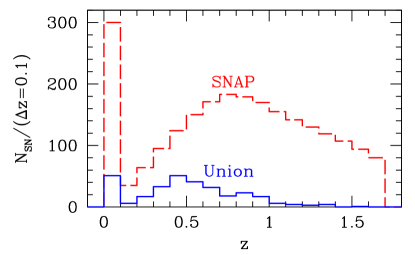
The Type Ia SN sample we use is the Union compilation SCP_Union . These SN observations measure relative distances, , over a range of redshifts spanning , with most SNe at (see Fig. 1). We include SN constraints using the likelihood code for the Union data sets Union_like , which includes estimated systematic errors in the covariance matrix SCP_Union .
For the current CMB data, we use the 5-year data release from the WMAP satellite Komatsu_2008 ; Nolta_2008 ; Dunkley_2008 employing the likelihood code available at the LAMBDA web site WMAP_like . Unlike the CMB priors used for the forecasts below, the likelihood used here contains the full information from the CMB angular power spectra, except for the small effects of gravitational lensing of the CMB that add little to current dark energy constraints from WMAP. We compute the CMB angular power spectra using the code CAMB Lewis:1999bs ; camb_url modified with the parametrized post-Friedmann (PPF) dark energy module PPF ; ppf_url to include models with general dark energy equation of state evolution where may cross .
II.2 SN and CMB Forecasts
For our SN forecasts, we take the expected redshift distribution for the SuperNova/Acceleration Probe (SNAP) KLMM_SNAP ; SNAP plus a low- sample of 300 SNe at . The SNAP magnitude errors include both statistical and systematic components:
| (1) |
where , shown in Fig. 1, is the number of SNe in each bin of width ( except for the statistical uncertainties in the low- SN bin, for which ), and is the width of the sub-bins used to smooth the distribution of SNe in redshift. We use 500 sub-bins up to . The second term on the right hand side of Eq. (1) models a systematic floor that increases linearly with up to a maximum at of mag per bin LinHut_highz .
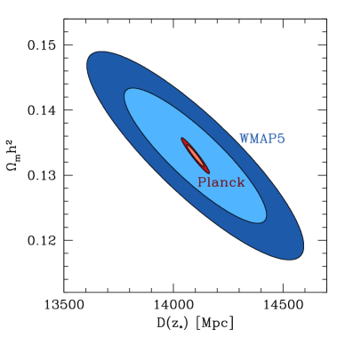
For the Planck CMB forecasts, we use a covariance matrix corresponding to the inner error ellipses in Fig. 2,
| (2) |
with parameters
| (3) |
Here is the comoving angular diameter distance to recombination.
In the Planck forecasts we ignore additional CMB information about dark energy such as the ISW effect and gravitational lensing of the CMB. Planck data are expected to obtain limits on the fraction of early dark energy of dePutter:2009kn ; Hollenstein:2009ph ; however, since these limits may depend on the modeling of early dark energy, we include in our forecasts only a conservative prior of (with fiducial value ) which approximates the current constraint from WMAP Doran .
II.3 Additional Priors
For both the current and forecasted constraints we add additional priors from recent measurements of baryon acoustic oscillations and the Hubble constant. The BAO constraint we use is based on the measurement of the correlation function of SDSS Luminous Red Galaxies (LRGs) Eisenstein , which determines the distance and expansion rate at through the combination . We implement this constraint by taking the volume average of this quantity, , over the LRG redshifts, , and comparing with the value of given in Ref. Eisenstein , (taking the scalar spectral tilt to be ). Using more recent BAO constraints, e.g. from Ref. Percival09 , has only a small effect on the current constraints with SN and CMB data PaperII .
We include the recent Hubble constant () constraint from the SHOES team SHOES , based on SN distances at that are linked to a maser-determined absolute distance using Cepheids observed in both the maser galaxy and nearby galaxies hosting Type Ia SNe. The SHOES measurement determines the absolute distance to a mean SN redshift of , which effectively corresponds to a constraint on for models with relatively smooth dark energy evolution in the recent past (cf. HubTrans ) such that . We implement this constraint as a measurement of km s-1 Mpc-1).
II.4 MCMC Methodology
Given the current or forecasted data, we use MCMC likelihood analysis (e.g. see Christensen:2001gj ; Kosowsky:2002zt ; Dunetal05 ) to determine dark energy parameter constraints and figures of merit for both the simple – models and general PC parametrization. From the likelihood of the data given each proposed parameter set , Bayes’ Theorem tells us the posterior probability distribution of the parameter set given the data
| (4) |
where is the prior probability density. The MCMC algorithm generates random draws from the posterior distribution. We test convergence of the samples to a stationary distribution that approximates by applying a conservative Gelman-Rubin criterion gelman/rubin of across a minimum of four chains for each model class. We use the code CosmoMC Lewis:2002ah ; cosmomc_url for the analysis of current data and an independent MCMC code for forecasts.
III Figure of Merit Comparisons
III.1 – Figure of Merit
We first consider the two-parameter model for the dark energy equation of state Linder_wa ; Chevallier_Polarski
| (5) |
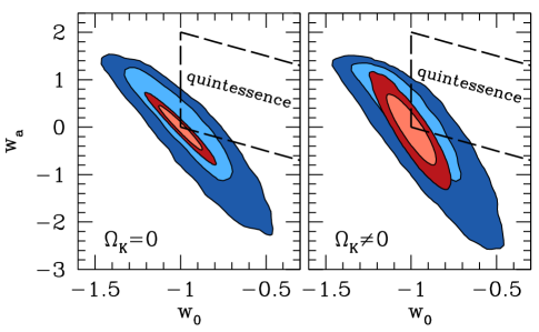
The FoM for this model defined by the Dark Energy Task Force DETF ; Huterer_Turner is the inverse of the area of the 95% CL region in the – plane. Figure 3 shows these regions for the current and forecasted data with and without marginalization of spatial curvature .
For a Gaussian error distribution, is proportional to the square root of the determinant of the 2D covariance matrix for and . Since the constant of proportionality used in practice for the FoM varies widely in the literature (e.g., see Bassett:2009uv ), we simply define
| (6) | |||||
The approximate equality between the two lines in Eq. (6) becomes exact for a Gaussian posterior distribution. Although the posterior in and is not perfectly Gaussian, the FoM computed using in Eq. (6) remains a good approximation to the area-based FoM. The difference between the two is in the worst case (current data with ) and in the other cases. Values of the version of are given in Table 1. The FoMs for current data are consistent with those found in previous studies of – constraints from similar data sets (e.g., Davetal07 ; Wright2007 ; Wang_FoM ; Mantz ).
| Data | ||||
|---|---|---|---|---|
| SNAP+Planck | 160 | 46 | 53000 | 19000 |
| Union+WMAP | 15 | 11 | 370 | 260 |
| ratio | 11 | 4.3 | 140 | 73 |
While analyses of – models typically allow to cross , it is useful to also consider a more restricted class of models that satisfy the quintessence bound in light of the PC description below. Imposing this quintessence prior greatly restricts the allowed parameter space as shown in Fig. 3. Assuming a flat (nonflat) universe, the FoM is a factor of (6.5) larger than without the quintessence prior for current data, and a factor of (9) larger for forecasts. Thus the addition of the quintessence prior increases the ratio of future to current values by about 60% (35%) relative to the ratios in Table 1. Note that the effect of the quintessence prior on the FoM for forecasts depends on the choice of the true model from which the data is drawn; for example, had we chosen fiducial and values that lie as far within the quintessence prior boundaries as the current data allow, the forecasted area allowed within the priors would be greater and the improvement in the FoM relative to current constraints would be smaller.
Even in this case where the posterior distribution with the quintessence prior is far from Gaussian, still approximates the area-based FoM through Eq. (6) reasonably well. Although values of the FoM are smaller by 35–40% than the area FoM, the ratio of future to current FoM values is nearly unchanged. We shall see that this type of agreement for quintessence models carries over to to the more general PC-based FoM in the next section.
| Union+WMAP | SNAP+Planck | ||||
|---|---|---|---|---|---|
| PC | |||||
| 1 | 0.375 | 0.061 | 0.041 | 0.011 | 0.008 |
| 2 | 0.421 | 0.087 | 0.132 | 0.037 | |
| 3 | 0.428 | 0.165 | 0.203 | 0.011 | 0.086 |
| 4 | 0.411 | 0.206 | 0.278 | 0.141 | |
| 5 | 0.450 | 0.184 | 0.278 | 0.206 | |
| 6 | 0.452 | 0.394 | 0.053 | 0.284 | |
| 7 | 0.425 | 0.360 | 0.117 | 0.343 | |
| 8 | 0.454 | 0.436 | 0.043 | 0.374 | |
| 9 | 0.461 | 0.438 | 0.418 | ||
| 10 | 0.463 | 0.026 | 0.448 | 0.424 | |
III.2 Principal Component Figure of Merit
We generalize the dark energy parametrization to allow arbitrary variations of the equation of state at with a basis of principal components (PCs) Hu_PC ; Huterer_Starkman . Details of the PC construction can be found in MHH1; here we highlight the points of special relevance for the FoM.
We construct the PCs based on the SN and CMB forecasts from Sec. II.2. The PCs are a set of orthogonal functions ordered by the precision with which they can be measured by the future SN and CMB data. Specifically, the principal component functions are eigenvectors of the SNAP+Planck covariance matrix in the space of piecewise constant values of the equation of state in redshift bins, . The principal components form a basis in which an arbitrary function may be expressed as
| (7) |
where are the PC amplitudes, is the number of redshift bins of width , and . We choose the maximum redshift for variations in to be , matching the largest redshift for the SNAP supernova data. The impact of dark energy evolution at higher redshifts is expected to be small, but perhaps non-negligible; to account for this possibility, we parametrize the equation of state at by a constant, . Likewise, we consider models with spatial curvature, . Note that and are not allowed to vary from their fiducial values of and , respectively, in the Fisher analysis used to construct the PCs.
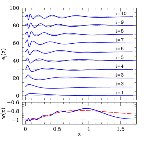
Since the highest-variance PCs correspond to modes of to which even future data are insensitive, we truncate the sum in Eq. (7) by replacing with . As shown in MHH1, the 10 lowest-variance PCs () form a basis which, for the classes of models we consider here, is sufficiently complete for the forecasts. Therefore, 10 PCs more than suffice for the current data as well. This set of basis functions is displayed in Fig. 4.
We impose priors on the PC amplitudes corresponding to the range of allowed for scalar field quintessence, following MHH1. Our conservative implementation excludes only parameter values that must violate these bounds even when considering possible compensation from the omitted higher-variance PCs (e.g. see the lower panel of Fig. 4 at ). This approach yields top hat priors of width
| (8) |
which follows from Eq. (A10) in MHH1.
In analogy to the – FoM in the previous section, we base the FoM for dark energy PCs on the determinant of the covariance matrix of for the lowest-variance PCs, . Even without informative data, this determinant is finite:
| (9) |
where the individual factors of (listed in Table 2) are the rms values of the corresponding top hat priors. These priors impact the FoM in a manner similar to those imposed in Ref. FoMSWG , where a Gaussian prior is adopted that requires the rms variation of for each PC mode, averaged over scale factor, to be no more than unity. However, our priors are slightly stronger since we use the quintessence bounds to impose a top hat prior on at all redshifts. In order that the FoM values do not reflect information that comes exclusively from the quintessence prior, we follow the convention in Ref. FoMSWG and renormalize the statistic to obtain
| (10) |
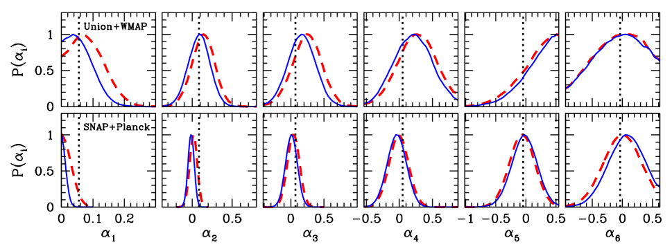
Table 2 shows the mean and rms of each of the 10 PCs from MCMC likelihood analysis using the current data and forecasts. Note that for components 6–10 in the current data the rms is dominated by the prior, and likewise for 7–10 in the forecast. Figure 5 shows the one-dimensional posterior probability distributions of the first 6 PCs where the information from the data resides.
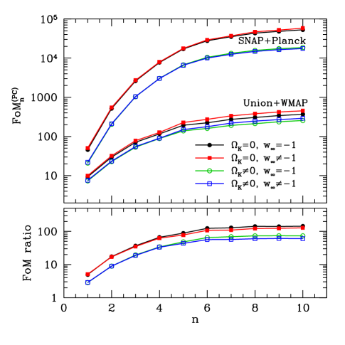
Figure 6 (upper panel) shows the FoM for the current data and forecasts. Note that for both data sets the FoM starts to saturate around the 6th PC as expected. The lower panel shows the ratio of FoMs of future and current data. Once again the saturation point is around the 6th PC with the total level of improvement varying from a factor of to depending mainly on whether spatial curvature is included.
This dependence of the FoM improvement on curvature is mainly due to a degeneracy between and the first PC which reduces the FoM when marginalizing over , particularly for the forecasts. This degeneracy is largely a consequence of our choice not to marginalize over when constructing the PCs, but the leading degeneracy between dark energy and curvature is included in the first PC. There is a related difference between the flat and nonflat cases in the – contours in Fig. 3 and in Table 1.
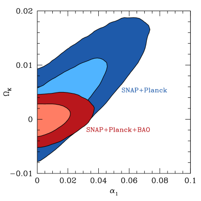
Current BAO and measurements (Sec. II.3) constrain enough that current SN+CMB PC uncertainties are affected little by curvature, but for the SN+CMB forecasts we need measurements of an absolute distance scale to achieve a FoM improvement comparable to that in the flat case. Figure 7 shows an example of breaking the – degeneracy using a 1% measurement at – as might be achieved from a future BAO experiment. As shown in Fig. 7 of MHH1, the shift in absolute distance corresponding to the curvature degeneracy is largely independent of redshift and its elimination could also be achieved with comparable measurements at from improved Hubble constant probes or from high-redshift BAO.
The small gap in ratios in Fig. 6 between models with and without early dark energy is driven by the current constraint on the 5th PC; as shown in Fig. 5, is not centered on zero and the distribution is cut off by the prior. Including early dark energy shifts this distribution further outside the prior, reducing the PC volume (and increasing the FoM) for current data. Forecasts for PCs are basically unaffected by early dark energy (see Fig. 6), so the overall effect of early dark energy is a slightly smaller FoM ratio when the 5th PC is included. This particular feature is not generic in the sense that it would not necessarily show up for other choices of data sets or dark energy parametrizations, but similar effects could appear in other analyses where the dark energy priors play an important role.
Since we are using the PCs constructed assuming the forecasted data rather than the current data, we could in principle have strong covariances between the PC amplitudes that would be hidden in Fig. 5. Likewise, we could have substantial differences between and definitions of the PC FoM involving ratios of Albrecht_Bernstein ; FoMSWG . In practice, however, the covariances between PC amplitudes remain small in all cases. Even for current data, the difference between and is for flat quintessence models and for nonflat models. The effect of covariances on the forecast FoM values is even smaller. Thus the 1D distributions in Fig. 5 accurately depict the current and future constraints on PC amplitudes.
A separate question is whether the use of gives misleading results due to non-Gaussianity of the PC posterior distributions (for example, due to distributions being cut off by the quintessence prior). To test the significance of such effects, we consider an alternate FoM analogous to the area-based FoM for – models,
| (11) |
where is the parameter subset consisting of the first PC amplitudes. The motivation of this form is that the allowed volume in parameter space is proportional to the inverse of the average number density of MCMC samples. The number density is proportional to , and the averaging over the posterior probability gives another factor of . The normalization of Eq. (11) is chosen so that for an D Gaussian posterior with covariance , .
For the 4–5 lowest-variance PCs, we find good agreement between and with differences of no more than . Using the FoM increases the ratio of future to current FoM values by 10–15%. For , accurate computation of the integral in Eq. (11) becomes more difficult due to the sparsity of MCMC samples.
Improvements in do not necessarily represent significant improvements in the ability to limit the parameter space of known dark energy models, especially for the higher PCs dePutter_Linder2 ; Barnard:2008mn . In order to address such issues, one can project the predictions of a model for onto the PC space and examine whether the predictions lie in the volume excluded by forecasted constraints. As an illustrative example, we consider a quintessence model with the potential
| (12) |
This model provides examples in the thawing class Caldwell_Linder for and can also mimic the low redshift behavior of Albrecht-Skordis models with oscillations around an offset minimum AlbSko00 . We consider an example where eV and with , and Hubble-drag frozen initial conditions ; the equation of state for this model is shown in the lower panel of Fig. 4. These parameters are chosen to be allowed by the current data but testable with future data.
Figure 5 compares the predictions for this model with the data constraints. Note that even for the future data only the first two PCs are stimulated at a level that the data can constrain. Thus for these types of models FoM is more representative of the parameter volume improvements than higher-dimensional FoMs. Taking into account the quintessence prior, the improvement from current to future data in this case is comparable to that implied by the – FoM.
More generally, studies have found that up to 3 PCs are useful for distinguishing amongst different commonly-used quintessence models with data sets comparable to our future forecasts Barnard:2008mn . On the other hand, these studies do not preclude the possibility that FoM improvements in the higher components can distinguish between other yet to be investigated classes of models.
IV Discussion
We have compared current and forecasted figures of merit (FoMs) for dark energy using both a simple – description of the equation of state, and a more complicated but more complete principal component (PC) parametrization. By consistently using a fixed set of PCs based on future data, and by generalizing the FoM definition to include possible parameter covariance, we showed how PC FoMs can be applied to likelihood analyses of both existing data sets and forecasts.
We have also shown that the covariance-based FoMs accurately represent relative changes in the parameter volume, even in the presence of strongly non-Gaussian posterior distributions such as those caused by imposing top hat priors. Traditional variance-based PC FoMs are consistent with those that include the full covariance for the cases we have tested, but we do not expect such agreement to hold in general. For example, if our PC eigenfunctions from SN and CMB data are applied to qualitatively different data, e.g. weak lensing or BAO, the FoMs that account for the parameter covariances should be employed.
For the – FoM, future space-based supernova data and CMB measurements from the Planck satellite can improve on current measurements by a factor of . For the PC FoM, the expected improvement is much greater still. While the forecasted precision for any single principal component is only a factor of 2–5 smaller than current uncertainties, the constraints on general quintessence models bounded by improve for approximately 6 components resulting in a reduction of the total allowed volume of dark energy parameter space by a factor of –. The FoM improvement depends mainly on whether or not variations in spatial curvature are allowed, with the maximum ratio of requiring either fixing the curvature with a theoretical prior () or combining future SN and CMB data with a measurement of absolute distance and/or the expansion rate with at least accuracy.
Although improvements from future SN and CMB data extend to 6 components of , many commonly-considered quintessence models are adequately described by the first three PCs for which the allowed volume only decreases by a factor of – relative to current measurements. While figures of merit provide a convenient model-independent metric to evaluate experiments, they must be interpreted with caution when science goals include discriminating amongst specific dark energy models.
Acknowledgments: MJM was supported by CCAPP at Ohio State; DH by the DOE OJI grant under contract DE-FG02-95ER40899, NSF under contract AST-0807564, and NASA under contract NNX09AC89G; WH by the KICP under NSF contract PHY-0114422, DOE contract DE-FG02-90ER-40560 and the Packard Foundation.
References
- (1) A. Albrecht et al., arXiv:astro-ph/0609591.
- (2) A. J. Albrecht and G. Bernstein, Phys. Rev. D75, 103003 (2007), [arXiv:astro-ph/0608269].
- (3) A. J. Albrecht et al., arXiv:0901.0721.
- (4) D. Huterer and M. S. Turner, Phys. Rev. D64, 123527 (2001), [arXiv:astro-ph/0012510].
- (5) Y. Wang, Phys. Rev. D77, 123525 (2008), [arXiv:0803.4295].
- (6) R. G. Crittenden, L. Pogosian and G.-B. Zhao, JCAP 0912, 025 (2009), [arXiv:astro-ph/0510293].
- (7) W. Hu, Phys. Rev. D66, 083515 (2002), [arXiv:astro-ph/0208093].
- (8) D. Huterer and A. Cooray, Phys. Rev. D71, 023506 (2005), [arXiv:astro-ph/0404062].
- (9) Y. Wang and M. Tegmark, Phys. Rev. D71, 103513 (2005), [arXiv:astro-ph/0501351].
- (10) C. Shapiro and M. S. Turner, Astrophys. J. 649, 563 (2006), [arXiv:astro-ph/0512586].
- (11) J. Dick, L. Knox and M. Chu, JCAP 0607, 001 (2006), [arXiv:astro-ph/0603247].
- (12) D. Sarkar et al., Phys. Rev. Lett. 100, 241302 (2008), [arXiv:0709.1150].
- (13) G.-B. Zhao, D. Huterer and X. Zhang, Phys. Rev. D77, 121302 (2008), [arXiv:0712.2277].
- (14) G.-B. Zhao and X.-m. Zhang, Phys. Rev. D81, 043518 (2010), [arXiv:0908.1568].
- (15) P. Serra et al., Phys. Rev. D80, 121302 (2009), [arXiv:0908.3186].
- (16) D. Huterer and G. Starkman, Phys. Rev. Lett. 90, 031301 (2003), [arXiv:astro-ph/0207517].
- (17) M. J. Mortonson, W. Hu and D. Huterer, Phys. Rev. D79, 023004 (2009), [arXiv:0810.1744], (MHH1).
- (18) M. J. Mortonson, W. Hu and D. Huterer, Phys. Rev. D81, 063007 (2010), [arXiv:0912.3816], (MHH2).
- (19) D. Huterer and H. V. Peiris, Phys. Rev. D75, 083503 (2007), [arXiv:astro-ph/0610427].
- (20) J. Tang, F. B. Abdalla and J. Weller, arXiv:0807.3140.
- (21) T. D. Kitching and A. Amara, arXiv:0905.3383.
- (22) R. de Putter and E. V. Linder, arXiv:0812.1794.
- (23) M. Barnard, A. Abrahamse, A. J. Albrecht, B. Bozek and M. Yashar, Phys. Rev. D78, 043528 (2008), [arXiv:0804.0413].
- (24) M. Kowalski et al., Astrophys. J. 686, 749 (2008), [arXiv:0804.4142].
- (25) http://supernova.lbl.gov/Union/.
- (26) E. Komatsu et al., Astrophys. J. Suppl. 180, 330 (2009), [arXiv:0803.0547].
- (27) M. R. Nolta et al., Astrophys. J. Suppl. 180, 296 (2009), [arXiv:0803.0593].
- (28) J. Dunkley et al., Astrophys. J. Suppl. 180, 306 (2009), [arXiv:0803.0586].
- (29) http://lambda.gsfc.nasa.gov/.
- (30) A. Lewis, A. Challinor and A. Lasenby, Astrophys. J. 538, 473 (2000), [arXiv:astro-ph/9911177].
- (31) http://camb.info/.
- (32) W. Fang, W. Hu and A. Lewis, Phys. Rev. D78, 087303 (2008), [arXiv:0808.3125].
- (33) http://camb.info/ppf/.
- (34) A. G. Kim, E. V. Linder, R. Miquel and N. Mostek, Mon. Not. R. Astron. Soc. 347, 909 (2004), [arXiv:astro-ph/0304509].
- (35) G. Aldering et al., arXiv:astro-ph/0405232.
- (36) E. V. Linder and D. Huterer, Phys. Rev. D67, 081303 (2003), [arXiv:astro-ph/0208138].
- (37) R. de Putter, O. Zahn and E. V. Linder, Phys. Rev. D79, 065033 (2009), [arXiv:0901.0916].
- (38) L. Hollenstein, D. Sapone, R. Crittenden and B. M. Schaefer, JCAP 0904, 012 (2009), [arXiv:0902.1494].
- (39) M. Doran, G. Robbers and C. Wetterich, Phys. Rev. D75, 023003 (2007), [arXiv:astro-ph/0609814].
- (40) D. J. Eisenstein et al., Astrophys. J. 633, 560 (2005), [arXiv:astro-ph/0501171].
- (41) W. J. Percival et al., Mon. Not. Roy. Astron. Soc. 401, 2148 (2010), [arXiv:0907.1660].
- (42) A. G. Riess et al., Astrophys. J. 699, 539 (2009), [arXiv:0905.0695].
- (43) M. Mortonson, W. Hu and D. Huterer, Phys. Rev. D80, 067301 (2009), [arXiv:0908.1408].
- (44) N. Christensen, R. Meyer, L. Knox and B. Luey, Class. Quant. Grav. 18, 2677 (2001), [arXiv:astro-ph/0103134].
- (45) A. Kosowsky, M. Milosavljevic and R. Jimenez, Phys. Rev. D66, 063007 (2002), [arXiv:astro-ph/0206014].
- (46) J. Dunkley, M. Bucher, P. G. Ferreira, K. Moodley and C. Skordis, Mon. Not. R. Astron. Soc. 356, 925 (2005), [arXiv:astro-ph/0405462].
- (47) A. Gelman and D. Rubin, Statistical Science 7, 452 (1992).
- (48) A. Lewis and S. Bridle, Phys. Rev. D66, 103511 (2002), [arXiv:astro-ph/0205436].
- (49) http://cosmologist.info/cosmomc/.
- (50) E. V. Linder, Phys. Rev. Lett. 90, 091301 (2003), [arXiv:astro-ph/0208512].
- (51) M. Chevallier and D. Polarski, Int. J. Mod. Phys. D10, 213 (2001), [arXiv:gr-qc/0009008].
- (52) B. A. Bassett, Y. Fantaye, R. Hlozek and J. Kotze, arXiv:0906.0993.
- (53) T. M. Davis et al., Astrophys. J. 666, 716 (2007), [arXiv:astro-ph/0701510].
- (54) E. L. Wright, Astrophys. J. 664, 633 (2007), [arXiv:astro-ph/0701584].
- (55) A. Mantz, S. W. Allen, D. Rapetti and H. Ebeling, arXiv:0909.3098.
- (56) R. R. Caldwell and E. V. Linder, Phys. Rev. Lett. 95, 141301 (2005), [arXiv:astro-ph/0505494].
- (57) A. Albrecht and C. Skordis, Phys. Rev. Lett. 84, 2076 (2000), [arXiv:astro-ph/9908085].