Cosmology in One Dimension: Fractal Geometry, Power Spectra and Correlation

Abstract

Concentrations of matter, such as galaxies and galactic clusters, originated as very small density fluctuations in the early universe. The existence of galaxy clusters and super-clusters suggests that a natural scale for the matter distribution may not exist. A point of controversy is whether the distribution is fractal and, if so, over what range of scales. One-dimensional models demonstrate that the important dynamics for cluster formation occur in the position-velocity plane. Here the development of scaling behavior and multifractal geometry is investigated for a family of one-dimensional models for three different, scale-free, initial conditions. The methodology employed includes: 1) The derivation of explicit solutions for the gravitational potential and field for a one-dimensional system with periodic boundary conditions (Ewald sums for one dimension); 2) The development of a procedure for obtaining scale-free initial conditions for the growing mode in phase space for an arbitrary power-law index; 3) The evaluation of power spectra, correlation functions, and generalized fractal dimensions at different stages of the system evolution. It is shown that a simple analytic representation of the power spectra captures the main features of the evolution, including the correct time dependence of the crossover from the linear to nonlinear regime and the transition from regular to fractal geometry. A possible physical mechanism for understanding the self-similar evolution is introduced. It is shown that hierarchical cluster formation depends both on the model and the initial power spectrum. Under special circumstances a simple relation between the power spectrum, correlation function, and correlation dimension in the highly nonlinear regime is confirmed.

1 Introduction

The observation that visible matter in the universe shows structure on a huge range of scales, from galaxies, to clusters, to super-clusters, to voids [1], has led Mandelbrot, Pietronero and others to conjecture that the structure of the universe may be fractal [2]. Support for this controversial conjecture is provided by the fact that the inter-galactic, two-body correlation function decays as a power-law [3]. If the geometry of the universe was truly fractal on all scales, then the basic principle of cosmology, that the universe is homogeneous and isotropic on large scales, would be violated. While current observations support the existence of an upper bound for the size of the largest structures, the issue is not completely closed [4, 5]. Typically, in nature, observable fractal behavior is usually restricted to a finite scale range [6]. Regardless of whether such a bound exists, it is still important to understand how the appearance of fractal geometry develops from the underlying dynamics.

The remarkable uniformity of the temperature distribution of the cosmic background radiation CMB is a consequence of the nearly uniform energy distribution at recombination [7]. Over time, the small (order $10^{-4}$) density fluctuations developed into the structures we see today. Measurements and theory suggest that, following inflation, the density fluctuations were Gaussian random variables with an approximate power-law spectral density. They were subsequently modulated by baryonic acoustic oscillation before recombination [3]. The commencement of structure formation in the dark matter component actually preceded recombination. These circumstances provide a natural scenario for the initial conditions of any dynamical study. With current technology astronomers can observe bright objects in the distant past. However, they cannot directly observe dynamical processes that take giga-years to unfold. As a consequence, computer simulation plays an especially prominent role in astrophysics, and has been employed to investigate complex behavior ranging from galaxy collisions and mergers to structure formation[8]. Although progress has been substantial, the ability of three-dimensional simulations with on the order of $10^{9}$ particles to resolve fractal scaling laws is still hampered by limited resolution and approximations in the underlying dynamics. In contrast, simulations with one-dimensional models can incorporate up to $10^{6}$ particles without compromising the two-body gravitational interaction. Thus, although they are less realistic “toy” models, they have the potential to yield insights into clustering with current computers. In addition, since theory suggests that the first collapsed objects were highly flattened “pancakes”, they may yet provide contact with the real universe [1, 9].

Rouet and Feix were the first to recognize the potential for using one-dimensional models to investigate clustering in a matter-dominated cosmological setting [10, 11]. Since there is no curvature in one dimension, general relativity does not provide a unique path for obtaining the correct laws of motion. Nonetheless, they showed how the transformation to co-moving coordinates could be accomplished in a completely self-consistent formulation which we refer to as the RF (Rouet-Feix) model. Starting with a spatially uniform initial distribution, they demonstrated that, as time evolved, hierarchical clustering occurs. Thus the one-dimensional evolution is similar to what is believed to have occurred in the universe following recombination. Rouet, Feix and Jamin computed the box counting dimension for the distribution of matter in the one-dimensional configuration and $\mu$ (position, velocity) space. They obtained a result of about 0.6 for the configuration space, strongly suggesting a fractal geometry. Since their seminal work, another similar model was proposed by Fanelli and Aurell, referred to simply as the quintic or Q model [12]. As we will see, the Q model sacrifices internal consistency in order to maintain the correct coefficient of the average cosmological density.

A different approach employing a one-dimensional model to explore matter-dominated cosmology was taken by Gouda and co-workers. Yano and Gouda employed the Zeldovich approximation [9] to investigate the evolution of the one-dimensional system[13]. When there is no cutoff in the initial spectra they showed that the evolution of the power spectra is self-similar, and established that three different scaling regimes occur, each with its own characteristic spectral index. Later Yano et al[14] studied the development of a single wave in the phase plane to investigate the effect of caustics on the evolution of the power spectra. In addition, Tatekawa and Meida used the Zeldovich approximation to study the self-similar evolution of a one-dimensional system with initial conditions selected from a Cantor set[15].

More recently Miller and Rouet extended the original work of Rouet and Feix to include an investigation of multi-fractal properties [16, 17]. They considered the fact that the clusters are actually forming in $\mu$ space. An analysis of the generalized fractal dimensions was applied to both configuration and $\mu$ space and it was shown that multifractal geometry develops in each. Miller and Rouet carried out a multifractal analysis of both the RF and Q models, as well as a Hamiltonian version. Valageas has investigated the Hamiltonian version with identical boundary conditions, and has shown the existence of a sequence of stationary and equilibrium states[18, 19]. The use of one-dimensional models has recently been extended by Sutter and Ricker to include a dark energy field in addition to dark matter [20]. They investigated how the introduction of dark energy influences the formation of Zeldovich “pancakes”, presumably the first large-scale structures to emerge in the cosmos. In a recent series of articles Gabrielli et alhave studied the one-dimensional system in the infinite particle limit [21, 22, 23, 24, 25]. A central focus of the series is the statistical properties of the force distribution obtained from sampling static distributions of particle positions from infinite perturbed lattices. In [23] a number of the issues mentioned here are discussed within this framework.

Theoretical cosmology suggests that during the period that density fluctuations remain small, evolution is linear and is dominated by a “growing mode” and the spectral distribution of the fluctuations remains a power-law [1]. However, in the simulations of Miller and Rouet described above, initial conditions were created by independently sampling the velocity of each particle from either a uniform or Gaussian distribution. In the work presented here, the initial conditions follow the cosmological picture for cold dark matter. We have performed simulations and a multi-fractal analysis of each model for a variety of initial, power-law, spectral densities. Here we describe the circumstances under which the evolution follows the accepted pattern of self-similar, hierarchical clustering. We show how the evolution of the spectral density and correlation function depend on both the model and the initial power-law index. We find that, for sufficiently large samples, the analytic relation between correlation dimension, correlation function, and spectral density is obeyed.

In the following we first explain the mathematical formulation of the different models in section 2. In particular, we show how to construct the exact gravitational potential and field for a one-dimensional, periodic system, i.e., Ewald sums for one dimension. In Section 3 we describe how simulations are performed and show how to create scale-free initial conditions for the growing mode in phase space for an arbitrary initial scaling index. We also present typical results for the Q model in the highly nonlinear region, including the calculation of power spectra and the two-body correlation function. In addition a simple analytic representation of the power spectra is introduced that captures the main features of the evolution, including the correct time dependence of the crossover from the linear to nonlinear regime and the transition from regular to fractal geometry. In Section 4 we introduce techniques for measuring generalized fractal dimensions and apply them to the Q model. In addition we give a comparison of results for related models and different initial power spectra and demonstrate that the power spectra, correlation function, and correlation dimension are interrelated in the nonlinear regime. To provide a physical basis for the observed behavior we introduce the mechanism of hierarchical virialization. Finally, in the last section, we present general conclusions that can be drawn from this investigation and provide a discussion of some open questions that still need to be addressed.

2 One-Dimensional Systems

Although dynamics in the universe is governed by the general theory of relativity, in a sufficiently small sample Newtonian dynamics provides an adequate working model [26]. In order to study structure formation, cosmologists focus on a segment of the universe $\Omega$ that is small enough that a Newtonian description is adequate, but much larger than the two-body correlation length [8]. They represent the location of the mass points of N-body simulations in comoving coordinates that follow the Hubble flow, so the average density remains constant. They ascribe a cubical shape to the sample and assert periodic boundary conditions to obtain a closed dynamical system that mimics a segment of the real universe [27]. This conserves mass and insures the continuity and smoothness of the gravitational potential and field at the boundaries. A potential problem is that, on the average, the universe is isotropic but the symmetry imposed by the cubical boundary conditions is not. For a large enough cube, this problem can be avoided for a finite time. In tree models Ewald sums are typically employed to compute the gravitational force from the infinite number of system “copies” [28] while in grid models the periodic boundary conditions are built into the potential [29].

A one-dimensional gravitational system corresponds to a set of parallel mass sheets moving in the direction perpendicular to their surface. In the seminal work of Rouet and Feix, they assumed a universe with spherical symmetry about a point. The elements of their universe were then concentric, spherical, irrotational mass shells. Far from the symmetry center, the radius of curvature is large and, locally, the shells are approximately planar and parallel. By choosing such a segment, they obtained a stratified system of comoving, planar, mass sheets for their model. However, if the object is to construct a consistent, one-dimensional, gravitational model that embraces an expanding background, it is not necessary to assume any special symmetry. One can just start with one dimension and assert a uniform expansion factor that also applies to the parallel dimensions of the mass planes. If gravity is the only force acting, then internal consistency forces the $t^{2/3}$ time dependence associated with the expansion factor of the Einstein de-Sitter, or matter-dominated, universe. However, the coefficient of the time-dependent mean density differs from the regular, three-dimensional model. To avoid this mild conundrum Fanelli and Aurell took a different approach. They first transformed to comoving coordinates in homogenous and isotropic three-space and then inserted a system of planes. Because the negative background density induced by the transformation to comoving coordinates doesn’t cancel with the average density associated with the mass sheets, an additional correction has to be included [17]. Here we will follow this approach.

Consider such a bounded region $\Omega$. We are interested in the evolution of density fluctuations following the time of recombination, so that electromagnetic forces can be ignored and Newtonian dynamics provides an adequate representation of the motion in a finite region [26]. Then, in a (3+1)–dimensional universe, the Newtonian equations governing a mass point are simply

$$\frac{d\mathbf{r}}{dt}=\mathbf{v,\qquad}\frac{d\mathbf{v}}{dt}=\mathbf{E}_{g}\mathbf{(r,}t\mathbf{)}$$ (1)

where, here, $\mathbf{E}_{g}\mathbf{(r,}t\mathbf{)\ }$ is the gravitational field. To follow the motion in a frame of reference where the average density remains constant, i.e. the comoving frame, we introduce the scale factor $A(t)$ for a matter-dominated universe [1] and transform to a new space coordinate which scales the distance according to $A(t)$. Writing $\mathbf{r}=A(t)\mathbf{x}$ we obtain

$$\frac{d^{2}\mathbf{x}}{dt^{2}}+\frac{2}{A}\frac{dA}{dt}\frac{d\mathbf{x}}{dt}+\frac{1}{A}\frac{d^{2}A}{dt^{2}}\mathbf{x=}\frac{1}{A^{3}}\mathbf{E}_{g}(\mathbf{x},t)$$ (2)

where, in the above, we have taken advantage of the inverse square dependence of the gravitational field to write $\mathbf{E}_{g}(\mathbf{x},t)=\frac{1}{A^{2}}\mathbf{E}_{g}\mathbf{(r},t)$ where the functional dependence is preserved. In a matter-dominated (Einstein-de Sitter) universe we find that

$$A(t)=\left(\frac{t}{t_{0}}\right)^{\frac{2}{3}},\qquad\rho_{b}(t)=\left(6\pi Gt^{2}\right)^{-1}$$ (3)

where $t_{0}$ is some arbitrary initial time corresponding, say, to the epoch of recombination, $G$ is the universal gravitational constant, and $\rho_{b}(t)$ is the average, uniform, density frequently referred to as the background density. The justification for equation (3) comes from the Robertson-Walker metric and the Friedman equation [1]. However, these results can also be obtained directly from equation (2) by noting that if the density is uniform so that all matter is moving with the Hubble flow, the first two terms in equation (2) vanish whereas the third term (times $A$) must be equated to the gravitational field resulting from the uniformly distributed mass contained within a sphere of radius $A\left|\mathbf{x}\right|$ which is simply the right-hand side of equation (2). Then the third term of equation (2) is the contribution arising by subtracting the field due to the background density from the uniform sphere [1]. Noting that $A^{3}\rho_{b}(t)=\rho_{b}(t_{0})$ forces the result. Alternatively, also for the case of uniform density, taking the divergence of each side of equation (2) and asserting the Poisson equation forces the same result. Thus the Friedman scaling is consistent with the coupling of a uniform Hubble flow with Newtonian dynamics [1].

In standard three-dimensional cosmological simulations it is common, but not ubiquitous, to employ conformal time, i.e to use A(t) as the measure of progress [29]. Here, for computational purposes, we will see that it is useful to obtain autonomous equations of motion with coefficients that do not depend explicitly on the time. This can be effectively accomplished [10, 11] by transforming the time coordinate according to

$$dt=B(t)d\tau,\qquad B(t)=\frac{t}{t_{0}}$$ (4)

yielding the autonomous equations

$$\frac{d^{2}\mathbf{x}}{d\tau^{2}}+\frac{1}{3t_{0}}\frac{d\mathbf{x}}{d\tau}-\frac{2}{9t_{0}^{2}}\mathbf{x=E}_{g}(\mathbf{x}).$$ (5)

These can be further simplified by choosing the inverse Jeans’ frequency $T_{J}$ for the unit of time [30]

$$T_{J}=\omega_{J}^{-1}=(4\pi G\rho)^{-1/2}=\sqrt{\frac{3}{2}}t_{o}$$ (6)

yielding

$$\frac{d^{2}\mathbf{x}}{d\tau^{2}}+\frac{1}{\sqrt{6}}\frac{d\mathbf{x}}{d\tau}-\frac{1}{3}\mathbf{x=E}_{g}(\mathbf{x)}$$ (7)

where we used the fact that $3t_{0}^{2}/2=1$ in the adopted time units and $\tau$ is now expressed in the new units. Thus equation (5) corresponds to a dissipative dynamical system in the comoving frame with friction constant $1/\sqrt{6}$ and with forces arising from fluctuations in the local density with respect to a uniform, three-dimensional, isotropic, neutralizing background.

We now imagine that the actual source of the density fluctuations is a system of parallel mass sheets with a neutralizing background, similar to a single-component plasma [31, 32]. For the special case of the stratified mass distribution induced by the one-dimensional system, the local particle density at time $t$ is given by

$$\rho(x,t)=\sum m_{j}(t)\delta(x-x_{j})$$ (8)

where $m_{j}(t)$ is the mass per unit area of the $j^{th}$ sheet and, from symmetry, the gravitational field only has a component in the $x$ direction. To avoid confusion, we will just refer to this as the mass. From Gauss’ law we know that the field due to a single mass sheet is constant. Then, for an isolated system with a finite number of particles and no background, the field experienced by one of the sheets is proportional to the difference between the mass on each side [33]. To obtain equations of motion, if we just take the component of equation (7) in the $x$ direction we see that a problem arises. The third term corresponds to the field from a sphere of constant density, but we now have a slab geometry so this term needs to be multiplied by a factor of three to maintain mass neutrality [17].

Following the three dimensional example, we will also assume periodic boundary conditions to approximate the actual behavior in a finite slab of our model one-dimensional universe for a finite time. The size of the system will be determined by the length of elapsed time we require to evolve the system before the presence of boundaries play a significant role. To accomplish this we need to determine the gravitational field induced by a single particle in the periodic system. Assume that the width, and hence the spatial period, of our system in the comoving frame is $2L,$ so we may choose the position $x_{1}$ of our particle of mass $m_{1}$ in $[-L,\>L)$ with the points at $L$ and $-L$ identified. For periodic boundary conditions the potential can only be defined for a mass-neutral system [29, 27, 28] where the source of the potential and field is the difference between the local density and its average over one period. Since our particle carries with it the negative background density $-m_{1}/2L$, the potential it induces, $\phi_{1}(x)$, satisfies the following Poisson equation

$$\frac{\partial^{2}\phi_{1}(x)}{\partial x^{2}}=4\pi m_{1}G[\delta(x-x_{1})-\frac{1}{2L}]$$ (9)

with the general solution

$$\phi_{1}(x)=2\pi m_{1}G[\left|x-x_{1}\right|-\frac{1}{2L}(x-x_{1})^{2}+b(x-x_{1})+c]$$ (10)

where $b$ and $c$ are constants.

The periodicity requirement, $\phi_{1}(L)=\phi_{1}(-L)$, forces $b=0$. In addition, to guarantee that as $L\rightarrow\infty$ the potential approaches that of the isolated system, we choose the arbitrary additive constant $c=0$, yielding for the final form of the potential

$$\phi_{1}(x)=2\pi m_{1}G[\left|x-x_{1}\right|-\frac{1}{2L}(x-x_{1})^{2}].$$ (11)

We immediately obtain the gravitational field $E_{1}$ induced by a single particle in the periodic system:

$$E_{1}(x)=-\frac{\partial\phi_{1}(x)}{\partial x}=2\pi m_{1}G\left[\frac{1}{L}(x-x_{1})+\Theta(x_{1}-x)-\Theta(x-x_{1})\right]$$ (12)

where $\Theta(x)$ is the usual step function and, for consistency, we assign $\Theta(0)=\frac{1}{2}.$ Note that we could have obtained the result from symmetry as well. Periodic boundary conditions in one dimension restrict the motion to the one-torus or circle. Since there is no preferred direction on the circle, the spatially averaged field must vanish. Thus symmetry alone guarantees that $b=0$. The results for the potential and field, equations (11,12) can also be obtained by employing a screening function to directly sum over the periodic system images, or replicas [34], and are effectively Ewald sums for one dimension. Unlike their three-dimensional analogs [28, 35], they have a simple closed-form expression.

Let us assume that the primitive cell of our periodic system contains $2N$ particles (sheets) confined within a slab with width $2L$, i.e. $-L\leq x<L$. For the special case of equal masses $m_{j}(t)=m(t)$, by direct summation the correct form of the gravitational field occurring at the location of particle $i$ in comoving coordinates is then

$$E_{g}(x_{i})=2\pi m(t_{0})G[\frac{2N}{L}(x_{i}-x_{c})+N_{R,i}-N_{L,i}]$$ (13)

since we already implicitly accounted for the fact that $m_{j}(t)=m(t_{0})/A^{2}$ in equation (5). In equation (13) $N_{R,i}$ ($N_{L,i}$) is the number of sheets on the right (left) of particle $i$ and $x_{c}(t)$ is the system center of mass in $[-L,\>L)$. The field is further simplified by establishing the connection between $m(t_{0})$ and the background density at the initial time, $\rho_{b}(t_{0}).$ Then

$$\rho_{b}(t_{0})=\left(6\pi Gt_{0}^{2}\right)^{-1}=\left(\frac{N}{L}\right)m(t_{0}),$$ (14)

and we may express the field by

$$E_{g}(x_{i})=\frac{1}{3t_{0}^{2}}\left(\frac{L}{N}\right)[\frac{2N}{L}(x_{i}-x_{c})+N_{R,i}-N_{L,i}].$$ (15)

The equations of motion for a particle in the system now read

$$\frac{d^{2}x_{i}}{d\tau^{2}}+\frac{1}{\sqrt{6}}\frac{dx_{i}}{d\tau}\mathbf{=}\left(\frac{1}{2}\right)[2(x_{i}-x_{c}(\tau))+N_{R,i}-N_{L,i}].$$ (16)

where we have taken account of the adopted unit of time (see equation (6)) and chosen the mean inter-particle spacing $L/N$ for the unit of length.

The description is completed by noting that, since the system satisfies periodic boundary conditions on the interval $[-L,\>L)$, when a particle leaves the primitive cell defined by $-L\leq x<L$ on the right (left), it re-enters at the left (right) hand boundary with the identical velocity. Note that from equation (13) there is no change in the field experienced by other particles during such a boundary crossing. This is a necessary condition for the one-torus geometry, since there is nothing special about this point. Other consequences of the torus geometry are discussed in [34]. In our simulations we made the further assumption of symmetry about the origin: For each particle with $0<x<L$ with velocity $v$, there is a twin located at $-x$ with velocity $-v$. With this stipulation, $x_{c}=0$ in equation (16) and the periodic boundary conditions are equivalent to an $N$-particle system with reflecting boundary conditions at $x=0,\,L$. For the times of interest, we demonstrated in [34] that the behavior of the system is nearly identical for each type of boundary. Note that, without the symmetry requirement, if one arbitrarily sets $x_{c}=0$ the torus geometry is violated.

As we mentioned earlier, by embedding the stratified system into a region of three-dimensional Euclidean space we are changing the local symmetry, so we have to adjust the local background density. In concept it is similar to the well-known Zeldovich approximation that is used to investigate the formation of the first matter concentrations that are believed to have a “pancake” geometry [1]. In their investigation of the structure of Zeldovich pancakes Aurell et alhave shown that the models are closely related [36]. In [23] it is argued that they are equivalent. Notice that this hybrid model mixes two different symmetries, the isotropic 3+1 dimensional system that cosmologists model with a periodic cube, and the planar geometry that is represented by a slab. Since the mass concentration in the idealized planes stretches to infinity in two directions it cannot represent the physical universe. The slab geometry can only represent cosmological evolution for a short time before the influence of the other dimensions (terms in the strain tensor) become important [1]. In contrast, the RF model is obtained from the reverse sequence where one first restricts the geometry to 1+1 dimensions and then introduces the transformation to the comoving frame. In this approach the derivation is more straightforward; it is not necessary to make the adjustment in the coefficient of $x_{i}$ as we did here to obtain the correct background contribution [10, 11, 16]. This is quickly seen by noting that the divergence of $\mathbf{x}$ is three times greater than the divergence of $x\boldsymbol{\hat{x}}$ which one would obtain by directly starting with the one-dimensional model. As a consequence, in the RF model, the coefficient of the first derivative term (the friction constant) in equation (16) is $1/\sqrt{2}$ instead of $1/\sqrt{6}$. In every other respect the models are identical. This simply illustrates that, since there is no curvature in a (1+1)-dimensional universe, there is a degree of arbitrariness in choosing the final model. It cannot be obtained solely from general relativity. For a discussion of this point, see Mann et al[37]. A Hamiltonian version can also be considered by setting the friction constant equal to zero. In their earlier work, using the linearized Vlasov-Poisson equations, Rouet and Feix carried out a stability analysis of the model without friction. They determined that the system followed the expected behavior, i.e., when the system size is greater than the Jeans’ length, instability occurs and clustering becomes possible [10, 11]. Of course, when the friction term is not present, both the Q and RF models are identical. Then, with the assumption that the friction term will not have a large influence on short-time linear stability, the analysis of the Hamiltonian version applies equally to both versions.

3 Simulations and Initial Conditions

An appeal of these one-dimensional gravitational systems is their ease of simulation. In each of the one-dimensional Newtonian models considered here (Q, RF and Hamiltonian), it is possible to analytically integrate the motion of the individual particles between crossings. Then the temporal evolution of the system can be obtained by following the successive crossings of the individual, adjacent, particle trajectories. In particular, for the Q model, if we let $y_{i}=x_{i+1}-x_{i}$, where we have ordered the particle labels from left to right, then we find that the differential equation for each $y_{i}$ is the same, namely

$$\frac{d^{2}y_{i}}{d\tau^{2}}+\frac{1}{\sqrt{6}}\frac{dy_{i}}{d\tau}-y_{i}=-1$$ (17)

The general solution of the homogeneous version of equation (17) is a sum of exponentials. By including the particular solution of the inhomogeneous equation (simply a constant) we obtain a fifth order algebraic equation in $u=\exp(\tau/\sqrt{6})$ for the successive crossings, defined by $y_{j}(\tau)=0$ ; hence the name Q, or quintic, model. These can be determined numerically in terms of the initial conditions by analytically bounding the roots and employing a numerical root-finding method. Note that for the RF model a cubic equation is obtained so the crossing times can be found analytically [10, 11, 16]. A sophisticated, event-driven algorithm was designed to execute the simulations. Using the Newton-Raphson method, the algorithm computes all possible crossings of adjacent pairs of particles with double-precision accuracy. Since, between crossings, the general solution of the dynamical equations is known analytically, once a crossing time is established, the position and velocity of each particle can be determined with the accuracy of the computer. Two important features of the algorithm are that it only updates the positions and velocities of a pair of particles when they actually cross, and it maintains the correct ordering of each particle’s position on the line. In contrast with typical N-body simulations, it is not necessary to introduce a discreteness length or time step. Using the algorithm we are able to carry out runs for significant cosmological times with large numbers of particles. In particular, it is possible to simulate a system until all of the mass is concentrated in just a few clusters. Depending on the initial conditions, this typically occurs on the order of 15-20 dimensionless time units into the simulation. Since, at this stage, the influence of the boundary conditions can no longer be ignored, there is no advantage in continuing the runs any further.

In cosmology, a consequence of inflation is that primordial density fluctuations are independent Gaussian random variables with a scale-free, power-law, spectral power distribution $P(k)\sim k^{n}$ [1]. Analysis of the WMAP measurements of the angular distribution of the CMB [7] yields a value for $n_{s}$ very close to unity, the Harrison-Zeldovich value. In this study we have investigated the dynamics of all three models with three different initial power spectra with indices, $n=0,\,1,\,2$. To construct the initial conditions we assume that the system is nearly uniform. If we use an ordered labeling of the $N$ particles, then the equilibrium positions are simply $x_{j0}=\frac{L}{N}(j-\frac{1}{2})$ for $j=1,...,N.$ Initially the system is in the linear regime and no crossings have occurred so the particles are assumed to be very close to their equilibrium points. Then, from equation (13) it is straightforward to show that the gravitational field on particle $j$ with position $x_{j}$ arising from the initial density fluctuation is, in our units, simply $\delta E(x_{j})=x_{j}-x_{j0}\equiv z_{j}$. Represent the local density fluctuation $\delta\rho(x)$ as a Fourier series with coefficients $\delta\rho_{k}$. Then, from the Poisson equation,

$$\delta E(x_{j})=-4\pi G\sum_{k}\frac{1}{ik}\delta\rho_{k}(e^{ikx_{j}}-1)$$

where we note that, at the origin, $\delta E$ vanishes and there is no contribution from $k=0$. Taking the Fourier coefficients as Gaussian random variables with a power-law power spectrum $\left|\delta\rho_{k}\right|^{2}$ of index $n$, we have $\delta\rho_{k}\sim k^{n/2}e^{i\theta_{k}}$ where the random phases $\theta_{k}$ are uniformly distributed on $\left[0,\,2\pi\right]$ and $\theta_{-k}$=$-\theta_{k}$ to insure $\delta\rho$ is real. Combining the above we obtain

$$z_{j}=x_{j}-x_{j0}=C\sum_{k>0}k^{n/2-1}[sin(kx_{j0}+\theta_{k})-sin(\theta_{k})],\quad\>k=\upsilon\pi/N,\>\upsilon=1,...,N$$

for the initial displacements of the particles from equilibrium. The sum is cut off when the wavelength is smaller than the mean inter-particle spacing. The constant of proportionality $C$ was chosen just small enough to prevent any crossings of the ordered positions. In the linear regime, from equation (16), the evolution of each particle is governed by

$$\frac{d^{2}z_{i}}{d\tau^{2}}+\frac{1}{\sqrt{6}}\frac{dz_{i}}{d\tau}=\delta E(x_{j})=z_{j}$$ (18)

with general solution

$$z_{j}(\tau)=a\exp\left(\frac{2}{\sqrt{6}}\tau\right)+b\exp\left(-\frac{3}{\sqrt{6}}\tau\right).$$

Following standard practice, we include only the contribution from the growing mode. This fixes the initial velocity of particle $j$ as $\frac{2}{\sqrt{6}}z_{j}$ and completes the assignment of the initial condition of the N-body system. For an alternative approach for indices $n=0,1,2$ see [21].

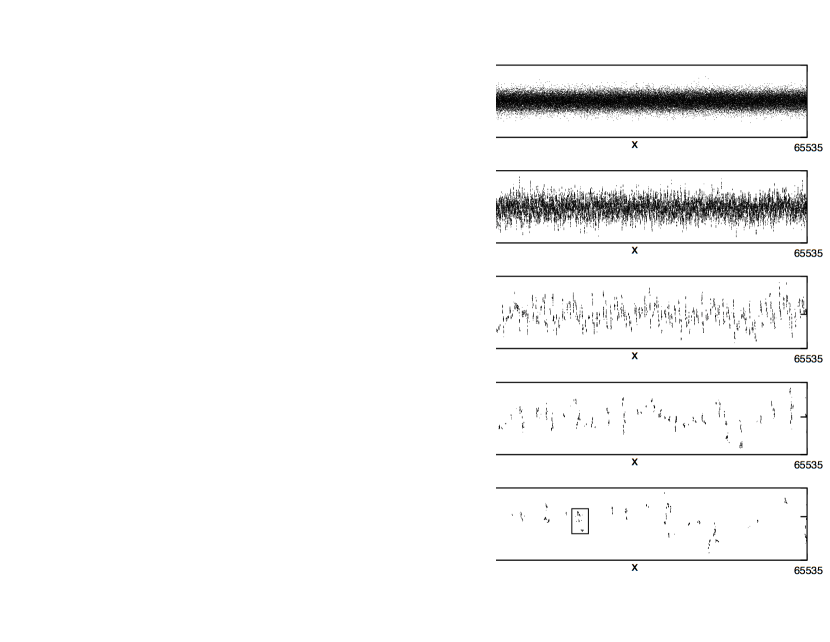
In figure 1 we present a visualization of a typical run with $2^{16}$ particles. The system consists of the Q model with an initial spectral index of $n=2$. Initially the velocity spread is small, within (-1, 1) in the dimensionless units employed here, and the system contains on the order of $10^{5}$ Jeans’ lengths. Of course, since the initial state does not represent thermal equilibrium, the Jeans’ length lacks predictive certainty, but strongly suggests that instability will ensue. Following the original work of Rouet et al[10, 11], we present a sequence of snapshots at integer values of the dimensionless scaled time through $\tau=18$. In the left column we present a histogram of the particle positions at increasing time frames, while on the right we display the corresponding particle locations in $\mu$ space. It is clear from the panels that hierarchical clustering is occurring, i.e., small clusters are joining together to form larger ones, so the clustering mechanism is “bottom-up”[1]. The first clusters seem to appear at about $\tau=8$ and there are many, while by $\tau=18$ there are only on the order of a dozen clusters. In larger simulations in the $\mu$ space we observe that, between the clusters, matter is distributed along linear paths [17]. As time progresses the size of the linear segments bridging the clusters increases. The behavior of these under-dense regions is governed by the stretching in $\mu$ space predicted analytically by Vlasov theory [16, 17]. Qualitatively similar histories are obtained for the RF model but the clustering occurs more slowly. However, there are some subtle differences. In figures 2 we zoom in and show magnified inserts from the mass distribution in $\mu$ space at time $\tau=18$. The hierarchical structure observed in these models suggests the existence of fractal geometry, but careful analysis is required to determine if this is correct.

Figure 1: Evolution in configuration and $\mu$ space for the quintic model with $2^{16}$ particles from $\tau=0$ to $\tau=18$. The initial distribution is such that the density power spectrum has a power-law of index $n=2$ (see Figure 3).

(a)

(a)

(b)

(b)

(c)

(c)

Figure 2: Consecutive expansions (zooms) in the $\mu$ space panels. Panel (a) shows the region selected by a rectangle in the $\mu$ space panels at $\tau=18$ of figure 1. Panel (b) is the region selected by a rectangle in panel (a) and so on. These representations have the appearance of a random fractal which suggests self-similarity.

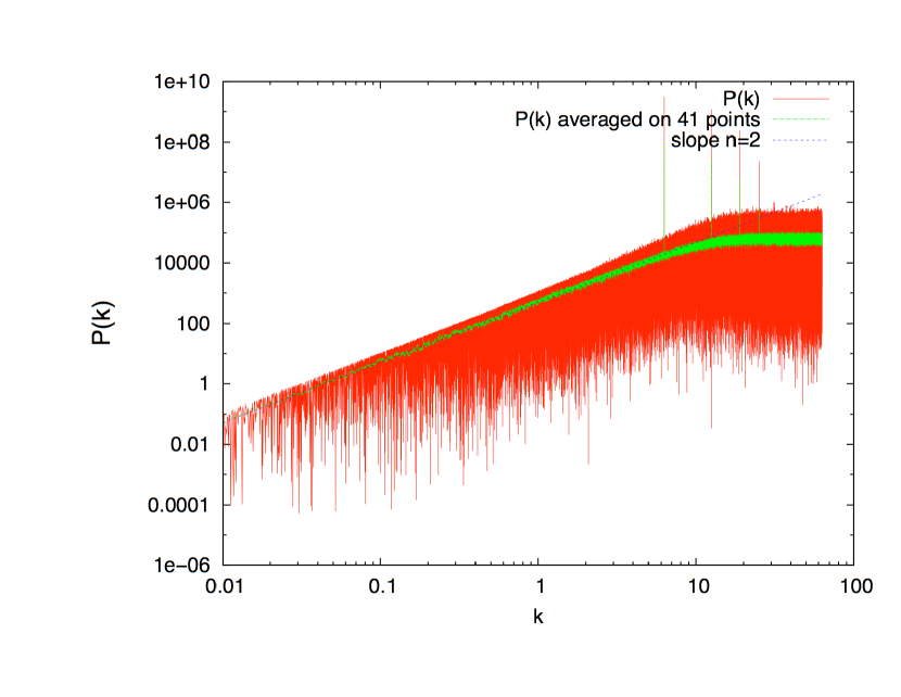
In figure 3 we show the power spectra of the initial density fluctuations $\left|\delta\rho_{k}\right|^{2}$. Although the data are noisy, by averaging over a group of neighboring points it is easy to extract the slope with good accuracy. Note that the graph conforms with the construction of the initial state described above. This confirms the validity of the initialization procedure. Note also that on small scales $(k>10)$ the slope flattens to $0$ showing that, for wavelengths less than the inter-particle spacing, the power spectra is simply a white noise as anticipated.

Figure 3: The Power spectrum of the initial density fluctuations for the quintic model. Particles have been distributed so that the power spectrum presents a power-law of index $n=2$.

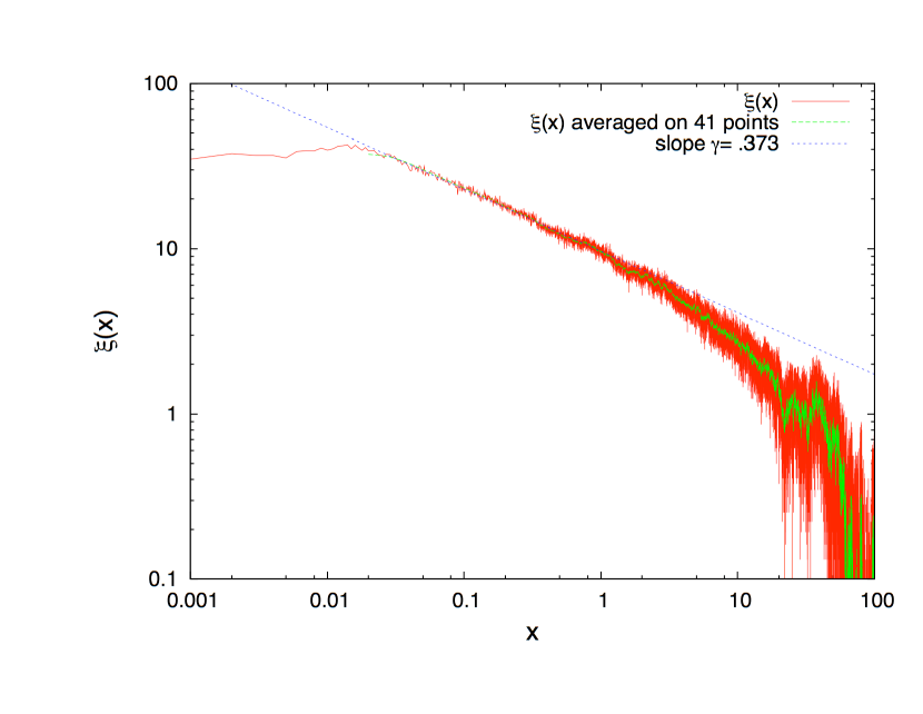
Historically, power-law behavior in the tail of the density-density correlation function has been taken as the most important signature of self-similar behavior of the distribution of galaxy positions [3, 38]. Even at $\tau=18$ we can see from the snapshots that the clusters are well developed, but still much smaller than the system size. Then it is safe to assume that boundary conditions do not yet play a significant role. In figure 4 we provide a log-log plot of the correlation function $\xi(r)$ at $\tau=13$ defined by

$$\xi(r)=\left\langle\delta\rho(x+r)\delta\rho(x)\right\rangle$$

$$\sim\frac{1}{\Delta}\int_{r}^{r+\Delta}\left[\sum_{i,j,i\neq j}\delta(r^{\prime}-(x_{i}-x_{j}))-\frac{N\left(N-1\right)}{2L^{2}}\right]dr^{\prime}$$ (19)

where particles $i$ and $j$ are such that $L/4<x_{i}<3L/4$ to avoid boundary effects, and $\Delta$ is the bin size. We observe three distinct regions in figure 4. First there is a relatively flat region at small scales. It is followed by a scaling region from about $0.02<r<2.0$, a range of about 2 decades, where $\xi(r)\propto r^{-\gamma}$, which finally deteriorates into noise. This is similar to cosmological studies which also exhibit the intra-cluster structure at small scales, and the inter-cluster scaling seen here. In addition, in the real cosmological setting, there is a peak due to baryonic acoustic oscillations [3]. The appearance of noise at larger scales occurs because the correlation function is decreasing while the noise is relatively constant. In a log-log plot, as $r$ is increased, at some point the noise becomes as large as the mean so large fluctuations appear in the data. Expressed differently, in a log-log plot of the correlation function, the apparent noise is effectively magnified with increasing $r$ until it dominates the mean. A straightforward linearization shows that the effective amplitude of the noise in $\ln C$ grows as $\exp(\gamma\ln r)$ while it is still relatively small. In principle it should be possible to reduce the noise by taking an ensemble average of $\xi(r)$ over many runs, and then computing the slope of $\ln\left\langle\xi(r)\right\rangle$. However, since we already employ $2^{16}$ particles, and the effective noise is growing exponentially with increasing $r$, this may only slightly extend the apparently noise-free region. By computing the slope $\gamma$ of the log-log plot in figure 4 we are able to obtain an estimate of the correlation dimension $D_{2}=1-\gamma$ for a one-dimensional system [39]. We find that $\gamma=0.373$ for a scaling region of about two decades in $l$. This suggests that the correlation dimension is approximately 0.63, which is in agreement within the standard numerical error with the multifractal analysis described below in some detail (see table 1).

Figure 4: The correlation function at $\tau=13$ for the quintic model. It exhibits a scaling region in $r$ from about 0.02 to about 2, a range of about 2 decades with a scaling exponent $\gamma=.373$.

Table 1: Exponent values for the three different models. For pure power law behavior $D_{2}=1-\gamma=-n$. For each system, $N=65535$ and, initially, $n=2$.

• Model	Time $T$	$\gamma$	$n$	$D_{2}$
  Q	$13$	.373	-.672	.623
  	$16$	.349	-.637	.628
  RF	$13$	.552	-.490	.478
  	$16$	.547	-.496	.500
  H	$13$	.173	-1.048	.862
  	$16$	.163	-.880	.853

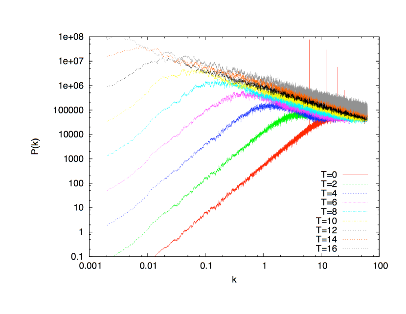
We have followed the evolution of the power spectra of the density fluctuations in these systems. In figure 5 we display log-log plots of $P(k)$ for a sequence of times. We see from the plot that two scaling regimes are present. For small $k$, i.e. on large scales, the system appears to retain the same dependence on $k$ as in the initial state and the linear regime. In contrast, using the same averaging method as earlier, we find that a second power law dependence develops at large $k$. At $\tau=13$ , for $k$ less than $.02$ to more than 50, i.e. over a range greater than three decades, this power-law behavior is clearly exhibited. As time progresses the division between the two regimes moves to the left so the shape is preserved and the process is self-similar. Between the two scaling regions is a transition region centered at, say, $k=k_{c}(\tau)$ which we define below. By $\tau=16$ there is no longer any trace of the linear regime. The behavior for $k<k_{c}$ is a remnant of the inter-cluster regions where the particles have not yet crossed. From Eq. (18) and the following discussion we see that the initial amplitude of deviations from the particle equilibrium positions in the growing mode is increasing as $\exp(2\tau/\sqrt{6})$ resulting in the corresponding power spectra in the linear region to increase as $\exp(4\tau/\sqrt{6})$. Analysis of the plots in Fig. (5) confirm this nicely. This amplification corresponds to the “stretching” in the low density regions of $\mu$ space predicted by Vlasov theory [16, 17]. It is well known, and discussed from a fluid picture elsewhere in the literature [1, 40, 25].

Notice that in Fig. (5), as a rough approximation, the power spectra in the nonlinear region has the form $P_{nl}(k)=Bk^{n}$ where $B$ is approximately constant and $n\simeq-.65$. Therefore, in both the linear and nonlinear regimes, the power spectra are well characterized. We can use this rough picture to extract useful information about the system evolution. According to the above, for the linear region we can write $P_{l}(k)=A\,\exp(\tau/\tau_{l})\,k^{n_{l}}\mbox{ }$where here $n_{l}=2$, for the quintic model $\tau_{l}=\sqrt{6}$/4, and $A$ is a constant. Equating $P_{l}(k_{c})=P_{nl}(k_{c})$ at the transition we find

$$k{}_{c}(\tau)=\left[\frac{B}{A}\right]^{\frac{1}{n_{l}-n}}\exp(-\tau/\tau_{l}(n_{l}-n)).$$ (20)

In practice, Eq.(20) describes the transition, defined as the intersection of the two power laws, remarkably well. Within the context of this model, $2\pi/k_{c}$ represents the size of the largest clusters at that epoch. If we further assume that the intra-cluster particle density remains roughly constant, then we also see that the number of clusters deceases approximately as $\exp(-\tau/\tau_{m})$ where $\tau_{m}=\tau_{l}(n_{l}-n)$ can be taken as a measure of the mean time between mergers.

We can also obtain insight into the fractal nature of the distribution of particles in configuration space from this simple model. From the Weiner-Khinchine Theorem [41], the correlation function $\xi(r)$ can be obtained from the Fourier transform of P(k):

$$\xi(r)=\frac{1}{2\pi}\int dk\,P(k)\,cos(kr).$$ (21)

Combining the contributions on either side of $k_{c}$ we obtain after a little algebra

$$\xi(r)=\frac{1}{2\pi}Bk_{c}^{1+n}\left\{\int_{0}^{1}du\,u^{2}cos(rk_{c}u)+\int_{1}^{\infty}du\,u^{n}\,cos(rk_{c}u)\right\}.$$ (22)

The correlation dimension is arguably the most robust of the class of generalized fractal dimensions (see below). We can obtain the correlation dimension by examining the average distribution of particles $C(R)$ in a ball of radius $R$ around a given particle [42, 39],

$$C(R) = \rho\int_{-R}^{R}dr(1+\xi(r))$$ (23)

$$=2\rho\left\{R+\frac{1}{2\pi}Bk_{c}^{n}\left[\int_{0}^{1}du\,u\,sin(Rk_{c}u)+\int_{1}^{\infty}du\,u^{n-1}\,sin(Rk_{c}u)\right]\right\}.$$ (24)

The correlation dimension is given by

$$D_{2}=\lim_{R\rightarrow 0}\frac{\ln C}{\ln R}=\lim_{R\rightarrow 0}\frac{1}{\ln R}\ln\left[R+\frac{B}{2\pi}\left(a_{l}k_{c}^{n+1}R+a_{nl}R^{-n}\right)\right]$$ (25)

where, in the above, $\rho$ is the average density, the second integral was expressed in terms of the incomplete Gamma function, only the lowest order contributions to $C(R)$ were included and $a_{l}$ and $a_{nl}$ are constants of order unity. We see that when $\tau\ll\tau_{m}/(n+1)$, i.e. early in the evolution, the linear term dominates and we anticipate that numerical analysis of the simulations will yield $D_{2}\simeq 1$ while, for late times, the last term, contributed by the nonlinear regime, is dominant and $D_{2}\simeq-n.$

Careful observation of the clusters in the phase plane suggests a possible mechanism for the hierarchical, bottom-up cluster formation. The large amplitude on small scales initiates a large collection of small clusters. Perhaps they are seeded on the caustics studied by Yano and Gouda[14]. Once these clusters virialize, they “freeze out” of the expansion and become the new “particles” for the next epoch of larger clusters [1]. In turn, these cluster “particles” virialize and merge and the process continually repeats until boundary effects interfere. At large scales $P(k)$ continues to increase as a result of the exponential growth in the remnants of the growing mode. On the other hand, at smaller scales, the freezing out of the clusters blocks the steady increase of $P(k)$. Thus virialization on successively larger scales determines the shape of the power spectra and qualitatively explains the observed results of the simulations. Since it is a renormalization process, the evolution is self-similar. Of course, it is a continuous process. The fact that larger “sub-clusters” become the particles for the next stage of virialization causes the clusters to grow in real space. In their study, Yano and Gouda [13] found three scaling ranges, the linear regime for large scales, a small intermediate range with an index of $-1$, and the third region which they deemed multi-caustic. They hypothesize that the power-law behavior is induced by the generation of caustics following the first crossings. The small regime, with $n=-1$, is associated with the period of single crossings. In our simulations we see hints of the intermediate regime in the transition regions of Fig. (5). In addition the index values we obtained for the behavior on small scales approximately correspond to theirs. Since Gabrielli et alhave argued that the Q model and the Zeldovich approximation are equivalent [23], this isn’t surprising. Additional discussion of the transition from the linear to nonlinear regime can be found in [40].

Figure 5: Plots of the Power spectrum at $\tau=0,2,4,6,8,10,12,14,16$ for the quintic model. Two scaling regions are observed separated by the transition from linear to nonlinear behavior.

4 Fractal Measures

It is natural to assume that the apparently self-similar structure that develops in the phase plane (see figure 1) as time evolves develops fractal geometry, but we will see that things are not so simple. In their earlier study of the RF model, Rouet, Feix and Jamin found a box counting dimension for the particle positions in $\mu$ space of about 0.75 for an initial water bag distribution (uniform on a rectangle in the phase plane) and a fractal dimension of about 0.57 in the configuration space (i.e., of the projection of the set of points in $\mu$ space on the position axis) [11]. As far as we know, Balian and Schaeffer were the first to suggest that the distribution of galaxy positions is consistent with a bifractal geometry [39]. Their idea was that the geometry of the galaxy distribution was different in the clusters and voids and, as a first approximation, this could be represented as a superposition of two independent fractals. Of course, their analysis was restricted solely to galaxy positions. Since the structures which evolve are strongly inhomogeneous, here we perform a multifractal analysis [43] of the configuration space.

The multifractal formalism shares a number of features with thermodynamics [43, 42]. To implement it we partitioned configuration space into cells of length $l$. At each time of observation in the simulation, a measure $\mu_{i}=N_{i}(t)/N$ was assigned to cell $i$, where $N_{i}(t)$ is the population of cell $i$ at time $t$ and $N$ is the total number of particles in the simulation. The generalized dimension of order $q$ is defined by [43]

$$D_{q}=\frac{1}{q-1}\lim_{l\rightarrow 0}\frac{\ln{C_{q}}}{\ln{l}},\quad C_{q}=\Sigma\mu_{i}^{q},$$ (26)

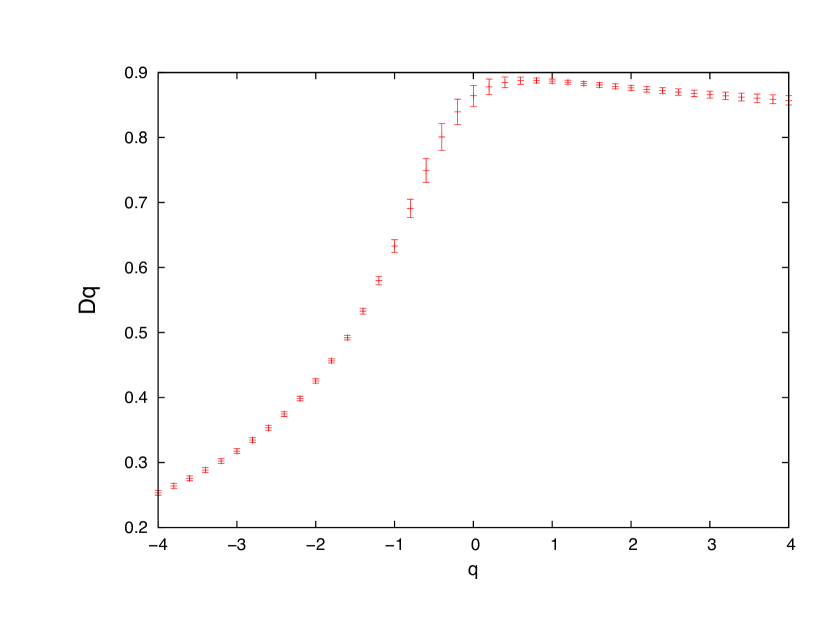
where $C_{q}(l)$ is the effective partition function [42], $D_{0}$ is the box counting dimension, $D_{1}$, obtained by taking the limit $q\rightarrow 1$, is the information dimension, and $D_{2}$ is the correlation dimension [43, 42]. As $q$ increases above $0$, the $D_{q}$ provide information on the geometry of cells with higher population, i.e. the regions of high density or clusters.

In practice, it is not possible to take the limit $l\rightarrow 0$ with a finite sample. Instead, one looks for a scaling relation over a substantial range of $\ln l$ with the expectation that a linear relation between $\ln C_{q}$ and $\ln l$ occurs, suggesting power-law dependence of $C_{q}$ on $l$. Then, in the most favorable case, the slope of the linear region should provide the correct power and, after dividing by $q-1$, the generalized dimension $D_{q}$. As a rule, or guide, if scaling can be found either from observation or computation over three decades of $l$, then we typically infer that there is good evidence of fractal structure [44]. Also of interest is the global scaling index $\tau_{q}$, where $C_{q}\sim l^{\tau_{q}}$ for small $l$. From Eq. (26 we see that $\tau_{q}$ and $f_{(}\alpha)$ are related to each other by $D_{q}(q-1)=\tau_{q}$ for $q\neq 1$ [42]. Here we present the results of our fractal analysis of the particle positions on the line (position only).

If it exists, a scaling range of $l$ is defined as the interval on which plots of $\ln C_{q}$ versus $\ln l$ are linear. Of course, for the special case of $q=1$, we plot $-\Sigma\mu_{i}\ln\mu_{i}$ vs $\ln l$ to obtain the information dimension [42]. If a scaling range can be found, $D_{q}$ is obtained by taking the appropriate derivative. It is well established by proof and example that, for a normal, homogeneous fractal, all of the generalized dimensions are equal, while for an inhomogeneous fractal, e.g., the Henon attractor, $D_{q+1}\leq D_{q}$ [43]. In the limit of small $l$, the partition function $C_{q}(l)$ can also be decomposed into a sum of contributions from regions of the inhomogeneous fractal sharing the same pointwise dimension $\alpha$,

$$C_{q}(l)=\int d\alpha\,l^{\alpha q}\rho(\alpha)\,l^{-f(\alpha)}$$ (27)

where $f\left(\alpha\right)$ is the fractal dimension of its support [43, 6, 42]. Then if, for a range of $q$, a single region is dominant, we find a simple relation between the global index $\tau_{q}$ and $\alpha$,

$$\tau_{q}=\alpha q-f(\alpha).$$ (28)

and a corresponding linear relation between $\ln C_{q}$ and $q$.

Initially the system is very cold, the $\mu$ space distribution of particles appears as a line, and the initial dimension is also about unity. In fact, initially the velocity of the particles is a perturbation. It is not large enough to allow particles to cross the entire system in a unit of time. After a while the fluctuations of force in the system destroys the approximate symmetry of the initial $\mu$ space distribution. Breaking the symmetry leads to the short-time dissipative mixing that results in the separation of the system into clusters. The behavior of the distribution of points in configuration space is similar. The initial dimension is nearly unity until clustering commences. At this time the dimensions in $\mu$ space and configuration space separate.

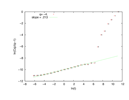
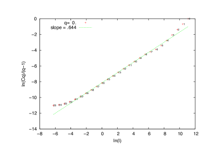
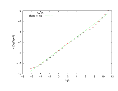
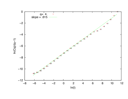
As time progresses, however, for the initial conditions discussed above, typically one dominant scaling region and a hint of a second develops. Of course this is in addition to the trivial scaling regions obtained for very small $l$, corresponding to isolated points, and to large $l$ on the order of the system size, for which the matter distribution looks smooth. The observed size of each scaling range depended on both the elapsed time into the simulation and the value of $q$. In some instances it was possible to find good scaling up to $4.7$ decades in $l$ !

In figure 6 we provide plots of $\frac{1}{q-1}\ln C_{q}$ versus $\ln l$ in configuration space for four different values of $q$ covering the range we investigated, ($-4<q<4$). To guarantee that the fractal structure was fully developed, we chose $\tau=16$ for the time of observation and the initial conditions are those given above. There was a basic consistency in the results with the largest dominant scale $-5.5<\ln l<6.5$ occurring for $q=4$ and the smallest, $-4<\ln l<4$, for $q=-4,$ i.e. from about $3.5$ to 5 decades. In all cases there was a hint of a second scaling region just beyond the primary, e.g. for $6.2<\ln l<7.6$ for the case $q=4.$ This scale corresponds to the turnover point in the power spectra. It appears to be a manifestation of the remnant of the linear region at large scales. The straight (dashed) lines that appear in the data are best curve fits obtained from linear regression for the range of the larger scaling region that is common to each of the values of $q$. Their slopes were used to compute the generalized dimensions.

(a)

(a)

(b)

(b)

(c)

(c)

(d)

(d)

Figure 6: Scaling behavior in configuration space at $\tau=16$ for the quintic model. Plots of $\frac{1}{q-1}{\ln{C_{q}}}$ versus $\ln{l}$ are provided for four values of q: a) q=-4, b) q=0. c) q=2, d) q= 4. The slopes have been determined using a linear regression from points 12 to 20.

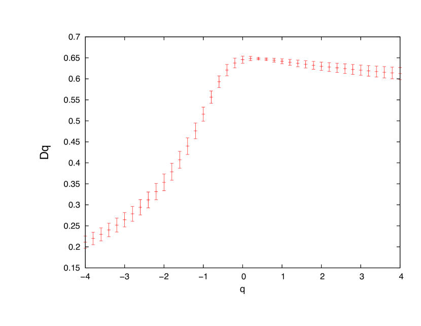
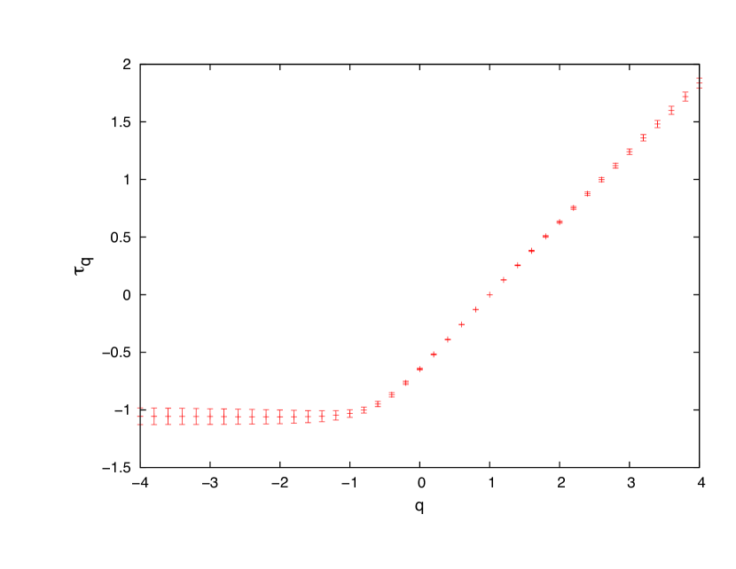
In figure 7 we illustrate the behavior of the generalized dimension $D_{q}$ for the configuration space of the quintic model at $\tau=16$ for $-4<q<4$. Although the embedding dimension is $d=1$, $D_{0}$ is about $0.65$ so the distribution is definitely fractal. For $q<0$ , the curve is an increasing function. This unphysical behavior suggests that there is simply a lack of sufficient data in the low-density regions to provide reliable dimensions. On the other hand, for $q>0$ , we see the decreasing behavior characteristic of a multifractal. In figure 8 we present a plot of $\tau_{q}$ vs $q$ constructed from the same data. Note the constant value for $q<0$. Comparison with equation (28) suggests that the pointwise dimension vanishes in the under-dense regions and that there is simply insufficient data to fix the type of geometry [42]. This is consistent with figure 7. For the case where $q>0$, the nearly linear behavior suggests that equation (28) applies here as well and yields a pointwise dimension $\alpha$ of about 0.65, and a support with Hausdorff dimension $f(\alpha)$ of about 0.7. It is not immediately obvious how to reconcile figures 7 and 8 for $q>0$ but it is interesting that both $\alpha$ and $f(\alpha)$ are very close to the value of $D_{0}$. In varying the initial conditions by selecting different random number seeds, there are slight variations in the overall picture. For $q>0$ we find $D_{q}$ consistently in the neighborhood $[0.62,\>0.65]$ but the degree of the multi-fractal nature, gauged by the negative slope in figure 7, varies somewhat. Perhaps the multifractal character suggested by the decrease of $D(q)$ with increasing $q$ is an artefact due to the increasing sparseness of denser and denser regions. However, since simulations of the RF model exhibit similar structure formation and a flat $D(q)$, this is doubtful.

Figure 7: Generalized dimension $D_{q}$ vs $q$ in configuration space for the quintic model at $\tau=16$.

Figure 8: Global scaling index $\tau_{q}$ vs. $q$ in configuration space for the quintic model at $\tau=16$.

Part of our goal is to compare how fractal geometry arises in a family of related models. So far we have presented results for the quintic, or Q, model. However we have also carried out similar studies of the Rouet-Feix (RF) model and the Hamiltonian model without friction (which can be obtained from either of the former by nullifying the first derivative contribution in equation (16)). In table 1 we compare the correlation dimension $D_{2}$ and the exponents generated by the power spectrum and correlation function for all three models at scaled times $\tau=13$ and $16$, where the clustering is highly developed. Writing $P(k)\sim k^{n}$ and $\xi(r)\sim r^{-\gamma}$, in principle there are simple relations between $D_{2}$, $n$, and $\gamma$ ; namely $D_{2}=1-\gamma=-n$. The first equality can be easily derived from the definition of correlation dimension (see e.g. [39, 42]and the discussion in the previous section), while the second is due to the Wiener-Khintchine theorem, i.e. the power spectrum is the Fourier transform of the correlation function [41]. We see from table 1 that these relations are approximately obeyed in these systems with $2^{16}$ particles. The agreement is superior for the Q and RF models. Experience has shown that, for them, as the system size is increased, so also is the agreement. While there are similarities in the fractal structure of the RF and Q models, they are not the same. For example in the quintic model the generalized fractal dimension $D_{q}$ is consistently greater than the corresponding dimension in the RF model showing that the inhomogeneity is stronger in the latter although the larger friction constant of the RF model causes clustering to commence later in the system evolution. Another difference is that plots of $D_{q}\>vs\>q$ for positive $q$ for the RF model are virtually constant, suggesting monofractal behavior. The values obtained for $n$ are consistent with those found in the simulations carried out by Yano and Gouda using the Zeldovich approximation in the “multicaustic” regime [13].

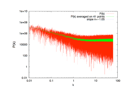
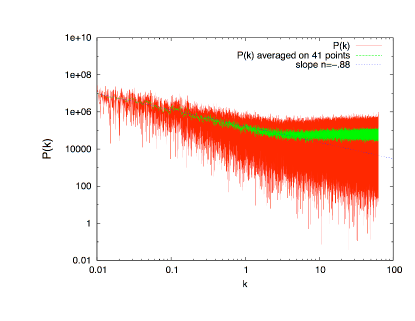
The Hamiltonian system was also investigated by Gabrielli et al[23]. Of the three models, it exhibits the most rapid cluster formation. However, in other aspects the behavior differs sharply from the dissipative systems. First, the scaling behavior is less robust. As shown in figures 9, plots of the power spectra at $T=13,\>16$ have a smaller scaling range. In addition, the fractal properties are much closer to an ordinary system. In figure 10 we see that the generalized dimensions $D_{q}\simeq 0.9$, much greater than the RF model, which presents the greatest structure with $D_{q}\simeq 0.5$. As can be seen in table 1, the connection between the exponents is weaker, no doubt due to the smaller scaling range. The relation between the exponents is only exact if the correlation function and power spectra are power-laws. Finally, if we extend the simulations beyond the time where boundary conditions can be neglected, say for $T>16$, we see a remarkable difference. For such times the matter distribution in the dissipative systems eventually collapses to just a single cluster. In contrast, as we see in figure 11, the Hamiltonian system becomes space filling. It appears to revert to the stationary state for this system introduced by Valageas [18, 19].

(a)

(a)

(b)

(b)

Figure 9: The Power spectrum for the Hamiltonian model : (a) at $\tau=13$ it exhibits a scaling region in $k$ from about 0.01 to 1, with a scaling exponent $-n=1.05$ (b) at $\tau=16$, the scaling range is [0.01;2], and $-n=0.88$.

Figure 10: Generalized dimension $D_{q}$ vs $q$ in configuration space for the Hamiltonian model at $\tau=16$.

Figure 11: Evolution in configuration and $\mu$ space for the Hamiltonian model with $2^{16}$ particles from $\tau=0$ to $\tau=20$. The initial distribution is such that the density power spectrum has a power-law of index $n=2$.

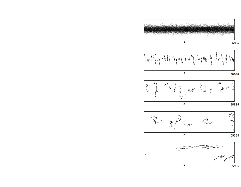
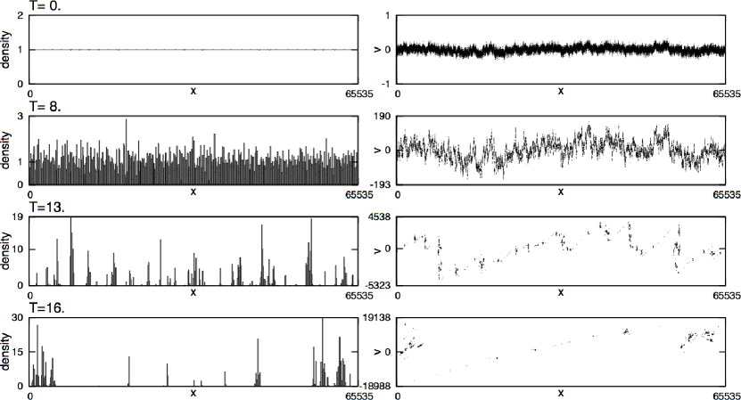
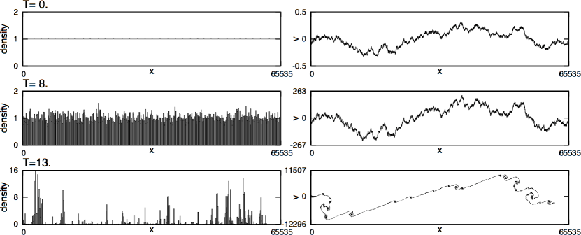
There is a sensitive dependence of the evolution on the initial conditions and, in particular, on the initial spectral index $n$. Although the cluster distributions in configuration space are similar, more information is available in the phase plane. We find that the smaller the initial index, the greater is the predominance of large clusters in the initial state, and these are very unstable. In figures 12 and 13 we show snapshots of the evolution of the Q model with $n=1$ and 0. We see from the figures that there is a strong correlation between the initial condition and the type of structure formation that develops. For the case where the initial particle distribution is white noise ($n=0$), examine the $\mu$ space snapshot at the time $\tau=13.$ Note that the system has not broken apart as we would expect from the simulations with $n=2.$ Moreover, the characteristic bottom-up behavior, where the smaller clusters combine to form larger ones as time evolves, is missing. Instead there is a single, large, connected, structure with a few small “subclusters” distributed within the pattern. Clearly hierarchical clustering is absent. Examining the snapshots for $n=1$ we see that the behavior is intermediate. Both small and large clusters are present, but the bottom-up scenario is not nearly as robust as for $n=2$. A clue for the origin of this behavior may be found in the work of Gabrielli et almentioned earlier [24, 25]. In their investigation of the statistical properties of static distributions of infinite systems that are on average uniform, they found that the variance of the force diverges if the structure factor is characterized by white noise ($n=0)$ and is marginal for $n=1$. Alternatively, the source of the behavior may arise from dynamical considerations. Energy at small scales is required to establish the presence of small clusters that can initiate a process of hierarchical virialization. For $n=0$ there is simply too much competition from large clusters and the hierarchical process is broken. Although the hierarchical process appears to start in a few locations, it doesn’t have sufficient time to develop. Long wavelengths drive the overall simulation.

Figure 12: Evolution in configuration and $\mu$ space for the quintic model with $2^{16}$ particles from $\tau=0$ to $\tau=16$. The initial distribution is such that the density power spectrum has a power-law of index $n=1$.

Figure 13: Evolution in configuration and $\mu$ space for the quintic model with $2^{16}$ particles from $\tau=0$ to $\tau=13$. The initial distribution is such that the density power spectrum has a power-law of index $n=0$.

5 Summary and Conclusions

Here and in our earlier work we have seen that hierarchical clustering is an intricate, highly choreographed dance in phase space that requires an initially cold and uniform system. The three models that were studied here differ only in the value of the friction constant, $\alpha$: $\alpha=$$\frac{1}{\surd 2,},$$\frac{1}{\surd 6,},0$ , respectively, for the RF, Q, and Hamiltonian models. The Q (Zeldovich) model has a hybrid geometry that may actually represent the local behavior of a 3+1 dimensional system for a short time, but cannot reproduce its real clustering properties in the highly nonlinear regime. Alternatively, the RF model is completely self-consistent with the transformation to comoving coordinates in 1+1 dimensions. It is useful for unambiguously studying nonlinear behavior, but has a weaker connection to the 3+1 dimensional universe. In fact, simulations of both the Q and RF models show remarkably similar behavior. The Hamiltonian model provides a contrasting dynamical system with no dissipation in the comoving coordinate system. Like the Q and RF models, it undergoes rapid hierarchical clustering for a short time span. However, unlike them, on long time scales the system becomes space filling and appears to revert to the stable stationary state investigated by Valageas [18, 19].

To mimic cosmological investigations, the initial positions were selected by sampling a power-law spectrum with random phases. The velocities were chosen to insure that the system is in the growing mode in phase space. The three models were studied with a range of initial power-law indices $n$. Qualitative behavior was observed for $n=3,4$ while extensive studies were carried out for $n=0,\>1,\>2$. Both the RF and Q models exhibited very similar behavior. For the case $n=2$, initially the systems remain fairly uniform. After some time, around $\tau=8$ for the Q model, the systems break into small clusters. As time progresses further the clusters coalesce into larger ones, supporting the well known bottom-up scenario of hierarchical cluster formation predicted for the real universe. Concurrently the variance of the velocities grows approximately exponentially. The power spectrum was monitored at various times and continued to show scale-free, power-law, behavior. In the strongly clustered epoch it turns around at small scales to a negative value supporting the observed structure of clusters of increasing size. It was shown that a simple analytic representation of the power spectra captured the main features of the evolution, including the correct time dependence of the crossover from the linear to nonlinear regime and the transition from regular to fractal geometry. The underlying mechanism for the observed behavior may be a process of “hierarchical virialization” whereby virialized clusters that have “frozen out” from the cosmic expansion become the new “particles” for the next virialization sequence. The measurements were consistent with the self-similar evolution found in the simulations of Yano and Gouda using the Zeldovich model [13].

In the well clustered regime, a multifractal analysis of the configuration space was performed. For the RF and Q models, in contrast with our earlier work with isothermal and waterbag initial conditions [16, 17], here a single dominant scaling range of the partition function $C_{q}$ was found for all values of $q$ considered. Generalized dimensions $D_{q}$ and scaling index $\tau_{q}$ were evaluated for $-4<q<4$. Robust fractal behavior was inferred for $q>0$ from the values of $D_{q}$. For the Q model the gradual decrease in $D_{q}$ for $q>0$ suggests that the system is also weakly multifractal. The RF model exhibited the greatest inhomogeneity. It appeared nearly monofractal with $D_{2}=0.5$. In addition, the two-body correlation function was constructed and also exhibited a power-law dependence on the displacement. For large samples, on the order of $10^{5}$ or more particles, the mathematical relation between the correlation dimension $D_{2}$, the spectral index $n$ and the correlation function decay exponent $\gamma$, $D_{2}=-n=1-\gamma,$ was nicely satisfied. For the Q model at $\tau=13$, $D_{2}=0.63$ over a finite scale range. For $n>2$ there was evidence of hierarchical clustering whereas for $n<2$ there was a tendency to form a few large clusters, but in the absence of self-similar, bottom-up, evolution. Like the Q and RF models, the Hamiltonian version undergoes rapid hierarchical clustering for a short time span. However, the scaling behavior was less robust, and the agreement among the exponents was weaker. In conclusion, one-dimensional models can exhibit the type of evolution characteristic of the real universe. Their evolution does reveal fractal behavior, but on a limited length scale that changes with time. It also shows that hierarchical structure formation depends sensitively on the initial conditions. Their three dimensional counterparts are useful for constraining models of the early universe.

A number of interesting questions about these models still remain. In forthcoming work we will explore the connection between symmetry and the various one-dimensional models and show how additional models analogous to the Q type can be constructed. We will also establish a connection between the increase in the variance of the velocity and virialization. While the fractal properties of the over-dense clusters appear to be well represented in the current work, the geometry of the under-dense “voids” has not been revealed. This is under investigation with a greater number of particles per cluster to improve the resolution. A complementary approach that may retain more information in the under-dense regions is provided by the numerical integration of the Vlasov equation. To finally address the conjecture of Balian and Schaeffer concerning the bifractality of the universe for this class of models, this must be completed. The approximate analytic representation of the power spectra introduced in Section (III) suggests that the low density inter-cluster regions have fractal dimension unity, but these results must be considered preliminary. A compelling issue is the connection between cosmologies in different dimensions. In an earlier work we showed that the RF model was able to crudely reproduce the time of galaxy formation in a matter-dominated universe [16]. It would be intriguing to be able to establish a more precise correspondence.

References

- [1] P. J. E. Peebles. Principles of Physical Cosmology. Princeton University Press, Princeton, NJ, 1993.
- [2] Yurij Baryshev and Pekka Teerikorpi. Discovery of Cosmic Fractals. World Scientific, Singapore, 2002.
- [3] V. J. Martinez. The large-scale structure in the universe: From power laws to acoustic peaks. Lect. Notes Phys., 665:269–289, 2009.
- [4] Paul Hunt and Subir Sarkar. Constraints on large-scale inhomogeneities from wmap5 and sdss: confrontation with recent observations. M.N.R.A.S., 401:547–588, 2010.
- [5] F. Sylos Labini, N. L. Vasilyev, and Y. V. Baryshev. Breaking the self-averaging properties of spatial galaxy fluctuations in the sloan digital sky survey – data release six. Astronomy & Astrophysics, 508:17–43, 2009.
- [6] Jens Feder. Fractals. Plenum, New York, 1988.
- [7] E. Komatsu et al. Five-year wilkinson microwave anisotropy probe (wmap) observations: Cosmological interpretation. Astrophysical Journal Supplement, 180:330–376, 2009.
- [8] V. Springiel, C. S. Frenk, and S. D. M. White. The large-scale structure of the universe. Nature, 440:1137, 2006.
- [9] S. F. Shandarin and Ya. B. Zeldovich. Reviews of Modern Physics, 61:185, 1989.
- [10] J.-L. Rouet, M. R. Feix, and M. Navet. Fractals in astronomy. In A. Heck, editor, Vistas in Astronomy 33, pages 357–370. Pergamon, 1990.
- [11] J.-L. Rouet, E. Jamin, and M. R. Feix. 1– spherically expanding universe. In A. Heck and J. M. Perdang, editors, Applying Fractals in Astronomy, pages 161–179. Springer-Verlag, Berlin, 1991.
- [12] D. Fanelli and E. Aurell. Astronomy & Astrophysics, 395:399, 2002.
- [13] Taihei Yano and Naoteru Gouda. Evolution of the power spectrum and self-similarity in the expanding one-dimensional universe. The Astrophysical Journal Supplement Series, 118:267–274, 1998.
- [14] Taihei Yano, Hiroko Koyama, Thomas Buchert, and Naoteru Gouda. Universality in the distribution of caustics in the expanding universe. The Astrophysical Journal Supplement Series, 151:185–192, 2004.
- [15] T. Tatekawa and K. Maeda. Astrophysical Journal, 547:531, 2001.
- [16] Bruce N. Miller and J. L. Rouet. Physical Review E, 65:056121, 2002.
- [17] Bruce N. Miller, Jean-Louis Rouet, and Emmanuel Le Guirriec. Fractal geometry in an expanding, one-dimensional, newtonian universe. Physical Review E, 76:036705, 2007.
- [18] P. Valageas. Thermodynamics and dynamics of a 1-d gravitational system. Astronomy and Astrophysics, 450:445 459, 2006.
- [19] P. Valageas. Relaxation of a one-dimensional gravitational system. Physical Review E, 74:016606, 2006.
- [20] P. M. Sutter and P. M. Ricker. Astrophysical Journal, 674:1, 2008.
- [21] Andrea Gabrielli. Point processes and stochastic displacement fields. Phys. Rev. E, 70:066131, 2004.
- [22] Andrea Gabrielli. Scale invariant forces in one-dimensional shuffled lattices. Physical Review E, 72:066113, 2005.
- [23] A. Gabrielli, M. Joyce, and F. Sicard. 1 - d gravity in infinite point distributions. Physical Review E, 80:041108, 2009.
- [24] A. Gabrielli and M. Joyce. Gravitational force in an infinite one-dimensional poisson distribution. Physical Review E, 81:021102, 2010.
- [25] Andrea Gabrielli, Michael Joyce, Bruno Marcos, and Francois Sicard. A dynamical classification of the range of pair interactions. arXiv:1003.5680[cond-mat.stat-mech], 2010.
- [26] Jai chan Hwang and Hyerim Noh. Why newtonian gravity is reliable in large-scale cosmological simulations. MNRAS, 367:1515, 2006.
- [27] Edmund Bertschinger. Simulations of structure formation in the universe. Annu. Rev. Astron. Astrophys, 36:599, 1998.
- [28] L. Hernquist, F. R. Bouchet, and Y. Suto. Application of the ewald method to cosmological n-body simulations. Astrophysical Journal Supplement, 75:231, 1991.
- [29] R. W. Hockney and J. W. Eastwood. Computer simulation using particles. Bristol: Hilger, 1988, 1988.
- [30] J. Binney and S. Tremaine. Galactic Dynamics. Princeton University Press, Princeton, NJ, 1987.
- [31] Elliott H. Lieb and Daniel C. Mattis. Mathematical Physics in One Dimension. Academic Press, New York, 1966.
- [32] Daniel C. Mattis. The Many-Body Problem: An Encyclopedia of Exactly Solved Models in One Dimension. World Scientific, Singapore, 1993.
- [33] K. R. Yawn and B. N. Miller. Incomplete relaxation in a two-mass one-dimensional self-gravitating system. Physical Review E, 68:056120, 2003.
- [34] Bruce N. Miller and Jean-Louis Rouet. Ewald sums for one dimension. Physical Review E, 82:066203, 2010.
- [35] S. G. Brush, H. L. Sahlin, and E. Teller. Monte carlo study of a one-component plasma. J. Chem. Phys., 45:2102, 1966.
- [36] E. Aurell, D. Fanelli, S. N. Gurbatov, and A. Y. Moshkov. Physica D, 186:171, 2003.
- [37] R. B. Mann and P. Chak. Statistical mechanics of relativistic one-dimensional self-gravitating systems. Physical Review E, 65:026128, 2002.
- [38] B. Jones, V. Martinez, E. Saar, and V. Trimble. Reviews of Modern Physics, 76:1211, 2004.
- [39] R. Balian and R. Schaeffer. Astronomy & Astrophysics, 226:373, 1989.
- [40] T. Baertschiger, M. Joyce, A. Gabrielli, and F. Sylos Labini. Gravitational dynamics of an infinite shuffled lattice of particles. Phys. Rev. E, 75:021113, 2007.
- [41] C. W. Gardiner. Handbook of Stochastic Methods, Second Edition. Springer-Verlag, Berlin, 1985.
- [42] Ed Ott. Chaos in Dynamical Systems, Second Edition. Cambridge University Press, Cambridge, UK, 2002.
- [43] T. C. Halsey, M. H. Jensen, L. P. Kadanoff, I. Procaccia, and B. Shraiman. Physical Review A, 33:1141, 1986.
- [44] J. L. McCauley. Physica A, 309:183, 2002.