Magnification Effects on Source Counts and Fluxes

Abstract

We consider the effect of lensing magnification on high redshift sources in the case that magnification varies on the sky, as expected in wide fields of view or within observed galaxy clusters. We give expressions for number counts, flux and flux variance as integrals over the probability distribution of the magnification. We obtain these through a simple mapping between averages over the observed sky and over the magnification probability distribution in the source plane. Our results clarify conflicting expressions in the literature and can be used to calculate a variety of magnification effects. We highlight two applications: 1. Lensing of high-$z$ galaxies by galaxy clusters can provide the dominant source of scatter in SZ observations at frequencies larger than the SZ null. 2. The number counts of high-$z$ galaxies with a Schechter-like luminosity function will be changed at high luminosities to a power law, with significant enhancement of the observed counts at $L\lower 2.15277pt\hbox{$\;\buildrel>\over{\sim}\;$}10\ L^{*}$.

1 Introduction

Magnification due to gravitational lensing leads to observable effects, namely changes in the number density of galaxies behind large-scale structure and galaxy clusters (known as magnification bias) and in the moments of the flux distribution due to unresolved sources at high redshift. These and other effects of lensing magnification have been studied extensively in the last few decades, usually assuming simple expressions that apply for constant magnifications.

In this brief note, we generalize to the case where magnification varies on the sky – the variation is taken to be given by a magnification probability in the source plane, while quantities of interested are observed as averages in the image plane. We apply this calculation to lensing of the intrinsic number count distributions of high redshift galaxies as well as moments of the flux for Poisson distributed high-$z$ galaxies behind galaxy clusters. Our goal is to provide the formulae needed for magnification effects in a variety of physical situations and give estimates of the scale of the main effects. Applications to more detailed models and results for Sunyaev-Zel’dovich surveys have been presented in a separate paper (Lima, Jain & Devlin 2009).

2 Constant Magnification

By definition, magnification (denoted $\mu$) is the Jacobian of the transformation between image (lensed) and source (unlensed) coordinates (e.g. Bartelmann & Schneider 2001). Along a given line of sight, its effect on differential solid angles is given by

$$d\Omega \rightarrow d\Omega_{\rm obs}=\mu d\Omega\,,$$ (1)

or $\mu=d\Omega_{\rm obs}/d\Omega$. We use subscript “$\rm obs$” for the observed (or lens plane or image plane) and no subscript for the (unlensed) source plane. The surface brightness of galaxy sources, defined as the flux per unit solid angle, is conserved by lensing. Since magnification increases the solid angle of sources by a factor $\mu$, it also increases their flux $S$ as

$$S \rightarrow S_{\rm obs}=\mu S\,.$$ (2)

In terms of the lensing shear $\gamma$ and convergence $\kappa$, the magnification is given by $\mu=1/[(1-\kappa)^{2}-|\gamma|^{2}]$.

As a result, the number density of a source population is modified by lensing magnification. Let $dn/dS$ denote the intrinsic number density per unit flux per unit steradian on the sky. Given a (constant) magnification $\mu$, it is modified as

$$\frac{dn}{dS}\rightarrow\frac{dn_{\rm obs}(S_{\rm obs})}{dS_{\rm obs}}=\frac{1}{\mu^{2}}\frac{dn}{dS}\left(\frac{S_{\rm obs}}{\mu}\right)\,.$$ (3)

The $1/\mu^{2}$ factor comes from transforming the angle $d\Omega$ and the flux differential $dS$ into their observed counterparts using Eqns. 1 and 2. The change in argument comes from the fact that the observed flux $S_{\rm obs}$ corresponds to true flux $S=S_{\rm obs}/\mu$.

Given the differential number density $dn/dS$, we may define the cumulative number density $n(>S)$, the average flux of the background galaxy population per steradian $\overline{\mathcal{S}}$ and the mean square flux per steradian $\overline{\mathcal{S}^{2}}$ as

$$n(>S) = \int_{S}\frac{dn}{dS^{\prime}}dS^{\prime}\,,$$ (4)

$$\overline{\mathcal{S}} = \int S\frac{dn}{dS}dS\,,$$ (5)

$$\overline{\mathcal{S}^{2}} = \int S^{2}\frac{dn}{dS}dS\,.$$ (6)

In the presence of a constant mangification $\mu$, the observed quantities are easily obtained using Eqns. 2 and 3 as:

$$n(>S)\rightarrow\frac{1}{\mu}n\left(>\frac{S_{\rm obs}}{\mu}\right),\ \ \ \overline{\mathcal{S}}\rightarrow\overline{\mathcal{S}},\ \ \ \overline{\mathcal{S}^{2}}\rightarrow\mu\ \overline{\mathcal{S}^{2}}.$$ (7)

Note that in the integrals over $S$ for $\overline{\mathcal{S}}$ and $\overline{\mathcal{S}^{2}}$ there is no upper or lower cutoff in flux.

There is a long history in the literature of magnification effects on source counts (starting with Canizares 1981, 1982 and Peacock 1982). The expressions above are consistent with those in the literature. We next consider the case of variable magnification on the sky.

3 Variable magnification on the sky

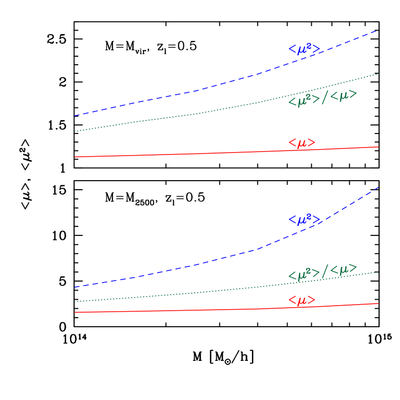
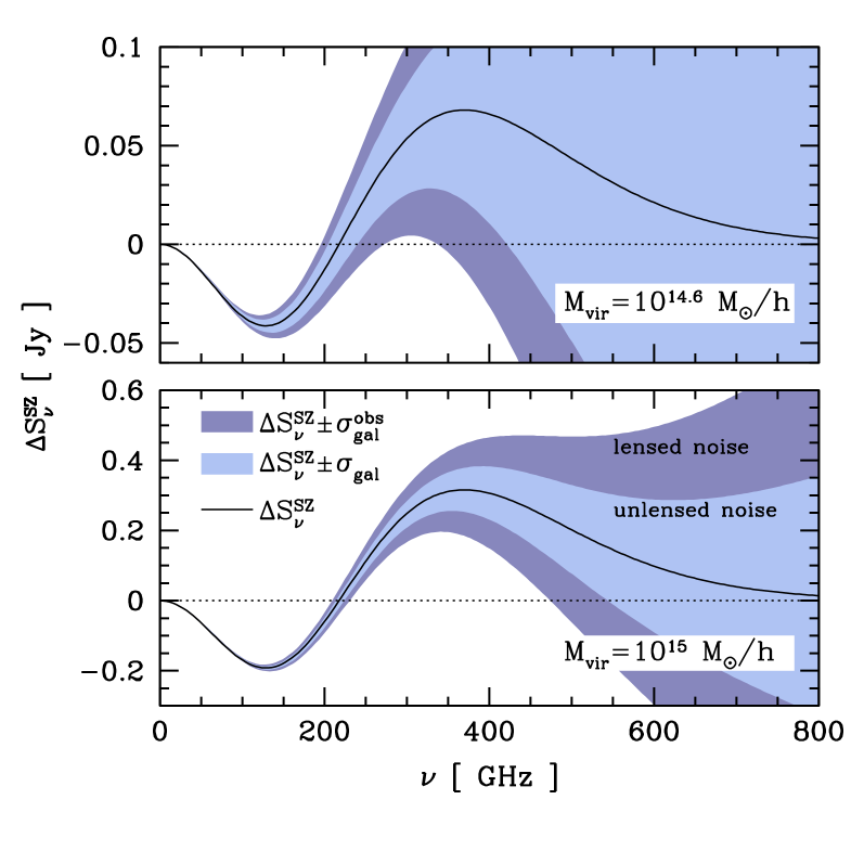
Figure 1: Left: Mean magnification $\langle\mu\rangle$ and mean squared $\langle\mu^{2}\rangle$ measured within clusters at redshift $z=0.5$ as a function of cluster mass. The upper panel averages within the virial radius of the cluster while the lower panel uses a smaller radius within which the overdensity is 2500 times the critical density. In X-ray and SZ analysis, different choices for the cluster radius are made which typically lie within these two. Right: Contamination of submillimeter galaxies to the SZ flux within the virial radius of clusters of virial mass $M_{\rm vir}=10^{14.6}$ and $10^{15}h^{-1}M_{\odot}$. The solid line shows the intrinsic SZ flux $\Delta S_{\nu}^{\rm SZ}$. The light shaded region delineate the 1-$\sigma$ region from contamination of submillimeter galaxies from Poisson noise in their counts, i.e. $\sigma_{\rm gal}^{2}=\overline{\mathcal{S}^{2}}_{\rm vir}$. The dark shaded region accounts for lensing magnification, which further enhances the noise by $\langle\mu^{2}\rangle/\langle\mu\rangle$, cf. Eqn 22.

We wish to generalize Eqns. 3 and 7 to the case that the magnification varies on the sky. This variation can occur over a large patch of the sky with fluctuations due to large-scale structure or simply over the surface of a galaxy cluster due to variations in the surface mass density and shear over this surface.

For variable magnification, the obvious step would be to average Eqns. 3 and 7 over the observed sky (i.e. the image plane), and this is indeed correct. Thus Eqn. 3 generalizes to $dn_{\rm obs}/dS_{\rm obs}=\int d\mu\ dn/dS\ P_{\rm obs}(\mu)/\mu^{2}$, where $P_{\rm obs}(\mu)$ is the normalized magnification probability in the image plane. It is often preferable to do calculations in the source plane. This is straightforwardly done by using the relation

$$P_{\rm obs}(\mu)=\frac{\mu}{\langle\mu\rangle}\ P(\mu)$$ (8)

where $P(\mu)$ is the source plane probability.

The above relation gives the generalized expressions:

$$\left\langle\frac{dn_{\rm obs}(S_{\rm obs})}{dS_{\rm obs}}\right\rangle = \frac{1}{\langle\mu\rangle}\int d\mu\frac{P(\mu)}{\mu}\ \frac{dn}{dS}\left(\frac{S_{\rm obs}}{\mu}\right)\,,$$ (9)

$$\langle n_{\rm obs}(>S_{\rm obs})\rangle = \frac{1}{\langle\mu\rangle}\int d\mu P(\mu)\ n\left(>\frac{S_{\rm obs}}{\mu}\right)\,,$$ (10)

$$\langle{\overline{\mathcal{S}}_{\rm obs}}\rangle = \overline{\mathcal{S}}\,,$$ (11)

$$\langle\overline{\mathcal{S}^{2}}_{\rm obs}\rangle = \frac{\langle\mu^{2}\rangle}{\langle\mu\rangle}\overline{\mathcal{S}^{2}}\,,$$ (12)

where $\langle\rangle$ denote averages of observed quantities over specified parts of the sky.

To obtain these results more formally, we evaluate the expressions on the LHS of the above equations by defining the average of a function $X$ in the image plane over an observed solid angle as

$$\langle X\rangle_{\rm obs}\equiv\frac{1}{\Delta\Omega_{\rm obs}}\int d\Omega_{\rm obs}X\,.$$ (13)

In the source (unlensed) plane the average over solid angle also defines $P(\mu)$

$$\langle X\rangle_{\rm source}\equiv\frac{1}{\Delta\Omega}\int d\Omega\ X\equiv\int d\mu P(\mu)\ X\,.$$ (14)

The function $X$ is a function of angle ${\bf\theta}$ on the sky through its dependence on $\mu({\bf\theta})$. Defining $P(\mu)$ on the source plane is conventional in lensing as it addresses questions such as, what is the fraction of sources that are magnified by a certain amount? Note that we have as desired

$$\int d\mu P(\mu) = \frac{1}{\Delta\Omega}\int d\Omega\ =1\,,$$ (15)

$$\int d\mu\ \mu P(\mu) = \frac{1}{\Delta\Omega}\int d\Omega\ \mu(\theta)\equiv\langle\mu\rangle=\frac{\Delta\Omega_{\rm obs}}{\Delta\Omega}\,.$$ (16)

In the limit of the whole sky, we have $\Delta\Omega_{\rm obs}=\Delta\Omega=4\pi$ and $\langle\mu\rangle=1$, i.e. the average magnification is unity.

Using the relations given above in Eqns. 13-16 for angular averaging, we can obtain Eqn. 9 as follows:

$$\left\langle\frac{dn_{\rm obs}(S_{\rm obs})}{dS_{\rm obs}}\right\rangle = \frac{1}{\Delta\Omega_{\rm obs}}\int d\Omega_{\rm obs}\frac{dn_{\rm obs}(S_{\rm obs})}{dS_{\rm obs}}$$

$$= \frac{1}{\langle\mu\rangle\Delta\Omega}\int d\Omega\ \mu\frac{1}{\mu^{2}}\frac{dn}{dS}\left(\frac{S_{\rm obs}}{\mu}\right)$$

$$= \frac{1}{\langle\mu\rangle}\int d\mu\ P(\mu)\frac{1}{\mu}\frac{dn}{dS}\left(\frac{S_{\rm obs}}{\mu}\right)\,.$$

This is our first desired result. It is obviously different from integrating the expression for $dn_{\rm obs}/dS_{\rm obs}$ from Eqn. 3 over $P(\mu)$ – doing that would have led to both factors of $1/\mu$ being inside the integrand. Next we substitute Eqn. 3 into

$$\langle n_{\rm obs}(>S_{\rm obs})\rangle=\frac{1}{\Delta\Omega_{\rm obs}}\int d\Omega_{\rm obs}\int_{S_{\rm obs}}\frac{dn_{\rm obs}(S_{\rm obs}^{\prime})}{dS_{\rm obs}^{\prime}}dS_{\rm obs}^{\prime}\,,$$

and change variables to $S^{\prime}=S_{\rm obs}^{\prime}/\mu$ to obtain Eqn. 10. Our expressions for number counts agree with Schneider (2006). Note that the unlensed number counts are independent of position on the sky, as are $\overline{\mathcal{S}}$ and $\overline{\mathcal{S}^{2}}$. Eqns. 11 and 12 for the observed flux moments can be obtained similarly and easily generalize to the $n$-th moment as $\langle\overline{\mathcal{S}^{n}}_{\rm obs}\rangle=\langle\mu^{n}\rangle/\langle\mu\rangle\ \overline{\mathcal{S}^{n}}$. This expression changes if there is a lower or higher limit to the integral over $S$. For instance in the case of an upper limit $S_{\rm cut}$, we can generalize to obtain

$$\overline{\mathcal{S}^{n}}_{\rm obs}(<S_{\rm cut})=\frac{1}{\langle\mu\rangle}\int d\mu\ P(\mu)\mu^{n}\ \overline{\mathcal{S}^{n}}\left(<\frac{S_{\rm cut}}{\mu}\right)\,.$$ (18)

Applications to galaxy clusters are discussed below. Another application is the contribution of unresolved point sources to CMB anisotropies, given by $C_{\ell}=\overline{\mathcal{S}^{2}}(<S_{\rm cut})$. The upper cutoff $S_{\rm cut}$ is usually introduced to remove resolved objects brighter than the cutoff. With lensing the observed contribution is enhanced – given by the above result with $n=2$. The enhancement depends on the slope of the $dn/dS$ relation at the cutoff. Finally we note that with a flux limit Eqn. 11 is no longer true, since surface brightness is only conserved when integrated over all fluxes.

4 Galaxy Clusters

Galaxy clusters produce magnifications ranging from $\sim 10$% enhancements above unity to factors of several or more as one approaches the critical curves. As a result both number counts of background galaxies and the flux moments of unresolved background sources are significantly altered.

Consider the unlensed average number of background galaxies within a cluster solid angle $\Delta\Omega_{\rm vir}$ defined by its virial radius, i.e. $N_{\rm vir}=\Delta\Omega_{\rm vir}\ n(>S)$. Notice that in the unlensed case $\Delta\Omega_{\rm vir}=\Delta\Omega$, i.e. the virial radius of the cluster is actually the intrinsic angle. With lensing the virial radius is now the observed solid angle, i.e. $\Delta\Omega_{\rm vir}=\Delta\Omega_{\rm obs}$, and we have

$$\langle N_{\rm obs}(>S_{\rm obs})\rangle_{\rm vir} = \Delta\Omega_{\rm vir}\langle n_{\rm obs}(>S_{\rm obs})\rangle$$

$$= \frac{1}{\langle\mu\rangle}\int d\mu P(\mu)\ N\left(>\frac{S_{\rm obs}}{\mu}\right)_{\rm vir}\,.$$

Note that $P(\mu)$ is now the magnification probability within the cluster virial radius (in the source plane as before). In the limit of constant magnification inside the virial radius we get $N_{\rm obs}=N/\mu$. Furthermore, if there is no lower limit to the flux integral $S_{\rm obs}\rightarrow 0$, we have $\langle N_{\rm obs}\rangle=N/\langle\mu\rangle$, i.e. we observe fewer galaxies in the line of sight of clusters. Note that our result for $N_{\rm obs}$ appears to differ from some of the literature (e.g. Schneider 2006), but the difference is that we use the same solid angle for the observed and unlensed case, because the only solid angle in town is the observed size of the galaxy cluster.

The intrinsic mean flux and mean square flux within the cluster solid angle $\Delta\Omega_{\rm vir}$ are $\overline{\mathcal{S}}_{\rm vir}=\Delta\Omega_{\rm vir}\ \overline{\mathcal{S}}$ and $\overline{\mathcal{S}^{2}}_{\rm vir}=\Delta\Omega_{\rm vir}\ \overline{\mathcal{S}^{2}}$. With lensing we have

$$\langle\overline{\mathcal{S}}_{\rm obs}\rangle_{\rm vir} = \Delta\Omega_{\rm vir}\langle\overline{\mathcal{S}}_{\rm obs}\rangle=\overline{\mathcal{S}}_{\rm vir}\,,$$ (20)

$$\langle\overline{\mathcal{S}^{2}}_{\rm obs}\rangle_{\rm vir} = \Delta\Omega_{\rm vir}\langle\overline{\mathcal{S}^{2}}_{\rm obs}\rangle=\frac{\langle\mu^{2}\rangle}{\langle\mu\rangle}\overline{\mathcal{S}^{2}}_{\rm vir}\,.$$ (21)

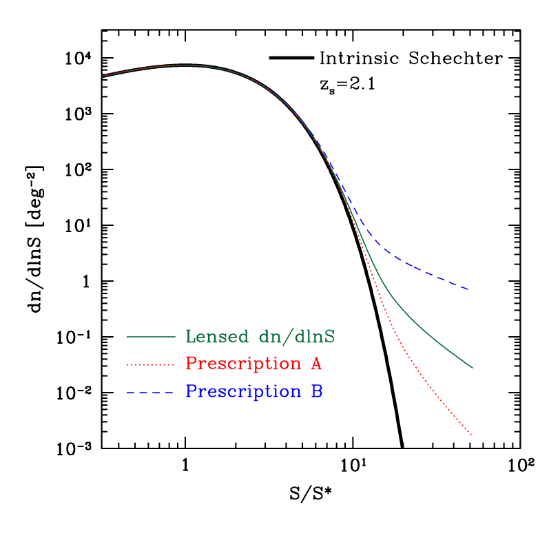
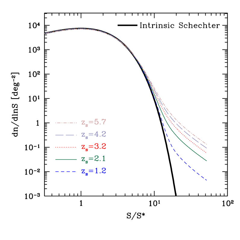
Figure 2: Left panel: Intrinsic and lensed galaxy number density ${\rm dn/dlnS}$ using different lensing prescriptions. The true underlying distribution is assumed to be of a Schechter type, which is then lensed by intervening halos. The solid (green) curves use Eqn. 9; the two alternatives shown (and described in Section 5.2) can change the predicted counts by an order of magnitude or more at the high luminosity end. Right panel: As above, but for different source redshifts.

Consider a cluster of observed radius 1 arcmin. The average flux from background galaxies crossing this 1 arcmin cluster is the same with or without lensing: with lensing, the background galaxies are brighter but less numerous and the two effects exactly compensate. So, lensing does not create a bias by increasing the expected flux within the cluster solid angle relative to a random 1 arcmin patch of the sky, as long as there is no flux cutoff.

For SZ surveys, the mean flux from background galaxies is subtracted in obtaining the SZ decrement or increment (depending on the observed frequency), but there is additional scatter due to the Poisson error from shot noise fluctuations (a given cluster having more or less galaxies than the expected average). This effect is important for SZ surveys, where high-$z$ submillimeter galaxies can contaminate the SZ signal (White & Majumdar 2004; Knox et al. 2004; Lima, Jain & Devlin 2009). Lensing enhances this source of scatter significantly, as the factor $\langle\mu^{2}\rangle/\langle\mu\rangle$ for galaxy clusters can be quite large – see Fig. 1. The estimates shown are based on an analytical model of cluster halos that uses NFW profiles and elliptical iso-potential contours (Lima, Jain & Devlin 2009). Our estimates are conservative in that we include cluster ellipticity but not substructure. Fig. 2 also indicates the error made in approximating moments of the flux by using the mean magnification (e.g. Refregier & Loeb 1997).

Notice that if we attempt to remove galaxies above some flux $S_{\rm cut}$, which could be removed if they were resolved, we introduce a difference between the observed and intrinsic average flux through the cluster, i.e. $\langle\overline{\mathcal{S}}_{\rm obs}\rangle\neq\overline{\mathcal{S}}$. In that case, the mean CMB flux is not equally contaminated by background galaxies and subtracting this mean flux from the cluster flux does not cancel the galaxy contribution on average. Therefore, removing bright galaxies from the sample biases the SZ signal. An observationally relevant situation arises if a flux cutoff is used to identify sources – thus altering both the number counts and flux contribution from unresolved sources (e.g. Refregier & Loeb 1997).

5 Illustrative number-magnitude relations

5.1 Power law

It is common in the magnification bias literature to consider the case of a local power law in the logarithm of the number counts. We then obtain for the observed cumulative number density:

$$n(>S)\propto S^{-\alpha}\ \rightarrow\ n_{\rm obs}(>S_{\rm obs})=\frac{\langle\mu^{\alpha}\rangle}{\langle\mu\rangle}\ n(>S_{\rm obs}).$$ (22)

Working with apparent magnitudes instead of fluxes this gives (using $m=-2.5{\rm log}_{10}S+{\rm Constant}$)

$$n(<m)\propto m^{s}\ \rightarrow\ n_{\rm obs}(<m_{\rm obs})=\frac{\langle\mu^{2.5s}\rangle}{\langle\mu\rangle}\ n(<m_{\rm obs}).$$ (23)

Note that the use of the power law for $n(>S)$ allows us to simplify the integral over $\mu$. The above equation agrees with the standard expression (e.g. Broadhurst, Taylor & Peacock 1995): $n_{\rm obs}(<m)=\mu^{2.5s-1}\ n(<m)$ for the case of constant magnification. For variable magnification, one needs to evaluate the averages as above. If one simply uses the factor $\langle\mu^{2.5s-1}\rangle$ behind a galaxy cluster instead of Eqn. 23, an error in the number counts can result. The error ranges from 3% for a cluster of mass $10^{14}\ h^{-1}M_{\odot}$ to 6% for a mass of $10^{15}\ h^{-1}M_{\odot}$. This would result in an equivalent bias in the inferred cluster mass. Mass estimates that rely on number counts may be feasible for large samples of clusters from future surveys.

To contrast the results from Eqn. 9 with other formulae used in the literature, consider first the naive generalization to variable magnification (which is correct in the image plane):

$${\rm\bf Prescription\ A:}\ \frac{dn_{\rm obs}(S_{\rm obs})}{dS_{\rm obs}}=\int d\mu\frac{P(\mu)}{\mu^{2}}\ \frac{dn}{dS}\left(\frac{S_{\rm obs}}{\mu}\right)\,.$$ (24)

This underestimates the lensing effect. Alternatively some authors drop the $\mu$ factors altogether (Paciga, Scott & Chapin 2009), which overestimates the lensing effect:

$${\rm\bf Prescription\ B:}\ \frac{dn_{\rm obs}(S_{\rm obs})}{dS_{\rm obs}}=\int d\mu P(\mu)\frac{dn}{dS}\left(\frac{S_{\rm obs}}{\mu}\right)\,.$$ (25)

5.2 Schechter luminosity function

A single power law number-magnitude relation is lensed into an observed relation with same power law (but different amplitude). However if the intrinsic $dn/dS$ is not a power law, then lensing changes the shape of the distribution as well. High magnification events shift galaxies with low fluxes to high fluxes – hence if $dn/dS$ falls sharply at high $S$, magnification can significantly enhance the counts at these fluxes.

We illustrate the effect of magnification for realistic galaxy populations by considering a Schechter function (Schechter 1976):

$$\frac{dn(S)}{dS} \propto \left(\frac{S}{S^{*}}\right)^{\alpha}e^{-S/S^{*}}\,.$$ (26)

For galaxies observed in a narrow redshift interval, such a $dn/dS$ relation can arise due to the Schechter luminosity function of the population.

In Fig. 2 we show the intrinsic distribution and the lensed versions according to the two incorrect prescriptions (denoted A and B) mentioned above, as well as the correct prescription of Eqn. 9. We assume all galaxies are at redshift $z_{s}=2.1$ and use a $P(\mu)$ obtained from N-body simulations by Hilbert et al (2007). We also choose $\alpha=0$ in the Schechter function. We plot $dn/d\ln S$ to relate more easily to the observational literature which shows number per unit absolute magnitude. Our results in Fig. 2 may be matched with high-$z$ luminosity functions by replacing $S/S^{*}$ with $L/L^{*}$.

The lensing contribution (correctly included in the green curves) is large for the Schechter function at the bright end ($S/S^{*}>10$). Thus for a population of galaxies with a Schechter luminosity function, the observed $dn/dS$ will not retain the exponential tail of the Schechter function. Using Eqn. 9 and approximating the Schechter function as having a sharp cutoff at $S=S^{*}$, it is easy to see that the integration over $\mu$ generates a power law in $dn/d\ln S$ whose slope is $-2$, due to the asymptotic slope $P(\mu)\propto\mu^{-3}$. The green solid curve approaches this slope beyond $S=10S^{*}$.

Choosing a lower (higher) value of $\alpha$ slightly enhances (suppresses) the lensing contribution at fixed $S/S^{*}$. Fig. 2 also shows that the difference between the three prescriptions is large at the bright end for the Schechter function. The $dn/dS$ in Fig. 2 is normalized so that the distribution matches submillimeter galaxies measured by the Balloon-borne Large Aperture Telescope (BLAST) (Devlin et al 2009) at $500$ $\mu$m. In a separate study we show that if the sub-mm galaxies lie at $z\sim 2-3$, then lensing of an intrinsic Schechter function can explain the observations from BLAST and other surveys (Lima, Jain, Devlin & Aguirre 2010).

Similar comparisons to luminosity function observations in the visible bands can be carried out: it is especially important to include lensing in the comparison of low-$z$ data with data at $z\lower 2.15277pt\hbox{$\;\buildrel>\over{\sim}\;$}1$ since the magnification contribution is significant only at high-$z$.

6 Discussion

We have derived expressions for computing average quantities in the observed image plane, given a distribution $P(\mu)$ of magnifications in the source plane. Our results, summarized in Eqns. 9-12, generalize expressions found in the lensing literature for the case of constant magnifications. We illustrated the effect of lensing on steep number counts of background galaxies and on boosting the contamination that high redshift galaxies induce in cluster SZ fluxes. The formulae we have presented may be useful for studying the intrinsic properties of high redshift galaxies and for current and upcoming cluster surveys.

The quantitative estimates presented here for galaxy clusters are based on analytical models of halos. While these incorporate realistic density profiles as well as halo ellipticity, they miss the full complexity of halo bimodality (due to major mergers) and substructure. These features only enhance the effects of averaging we have considered.

Finally we note that the lensing effects discussed here do not impact the predicted (magnification induced) cross-correlation of number counts measured in different redshift bins (Moessner & Jain 1998). Such cross-correlations depend on the two-point cross-correlations of magnification with the galaxy density. Thus measurements of magnification bias from galaxy-quasar cross-correlations or of its contaminating effect on high-$z$ ISW cross-correlations are unaffected by the spatial averaging issues discussed here.

Acknowledgments: We thank Anna Cabre, Yan-Chuan Cai, Mark Devlin, Mike Jarvis and Ravi Sheth for helpful discussions, and Stefan Hilbert for sharing his simulation results. We especially thank Gary Bernstein and Peter Schneider for sharing their insights and knowledge of the history of the field. This work was supported in part by an NSF-PIRE grant and AST-0607667.

References

- [1] Bartelmann, M., & Narayan, R. 1995, ApJ, 451, 60
- [2] Bartelmann, M., & Schneider, P. 2001, Phys. Reports, 340, 291, Section 4.4
- [3] Broadhurst, T. Taylor, A., Peacock, J. 1995, ApJ, 438,49.
- [4] Canizares, C. R. 1981, Nature, 291, 620
- [5] Canizares, C. R. 1982, ApJ, 263, 508
- [6] Devlin, M. J., et al. 2009, Nature, 458, 737
- [7] Hilbert, S., White, S. D. M., Hartlap, J., & Schneider, P. 2007, MNRAS, 382, 121
- [8] Lagache, G., et al. 2004, Ap. J. Supp., 254, 112
- [9] Lima, M., Jain, B., & Devlin, M. 2009, MNRAS, submitted, arXiv:0907.4387
- [10] Lima, M., Jain, B., Devlin, M. & Aguirre, J. 2010, arXiv:1004.4889
- [11] Moessner, R., & Jain, B. 1998, MNRAS, 294, L18
- [12] Paciga, G., Scott, D., & Chapin, E. L. 2009, MNRAS, 395, 1153
- [13] Peacock, J. A. 1982, MNRAS, 199, 987
- [14] Refregier, A., Loeb, A., 1997, ApJ, 478, 476
- [15] Schechter, P. 1976, ApJ, 203, 297
- [16] Schneider, P., 1987, A&A 179, 80
- [17] Schneider, P., 2006, “Saas-Free Advanced Course on Gravitational Lensing: Strong, Weak and Micro”, p. 59.
- [18] Takada, M., & Hamana, T. 2003, MNRAS, 346, 949