1 Introduction and Overview

While the prime example of the AdS/CFT correspondence is the duality between four-dimensional $\mathcal{N}=4$ super Yang–Mills theory (SYM) and type IIB superstring theory on $\mathrm{AdS}_{5}\times\mathrm{S}^{5}$ [1, 2, 3], another remarkable instance equates $\mathcal{N}=6$ superconformal Chern–Simons theory in three dimensions (SCS) and type IIA strings on $\mathrm{AdS}_{4}\times\mathrm{\mathbb{C}P}^{3}$ [4]. In the study of the spectrum on both sides of these two correspondences, the discovery of integrability [5, 6, 7, 8, 9, 10, 11, 12, 13, 14, 15, 16, 17, 18, 19, 20, 21, 22, 23] in the planar limit has been of crucial importance, and has lead to the belief that the planar theories might be exactly solvable.

Exact solvability would suggest that integrability also manifests itself in the scattering amplitudes of the above theories. For the $\mathrm{AdS}_{5}$/$\mathrm{CFT}_{4}$ correspondence, this is indeed the case. Motivated by a duality between Wilson loops and scattering amplitudes in $\mathcal{N}=4$ SYM theory [24, 25, 26, 27], a dual superconformal symmetry of scattering amplitudes was found at weak coupling [28, 29, 30, 31]. This dual symmetry can be traced back to a T-self-duality of the $\mathrm{AdS}_{5}\times\mathrm{S}^{5}$ string background [32, 33] (see also [34] for a review). In addition to the standard superconformal symmetry, the dual realization acts on dual momentum variables leaving all $\mathcal{N}=4$ SYM tree-level amplitudes invariant [35]. Integrability at weak coupling then arises as the closure of standard and dual superconformal symmetry into a Yangian symmetry algebra for tree-level scattering amplitudes [36]. In fact, $\mathcal{N}=4$ SYM tree-level amplitudes seem to be uniquely determined by a modified Yangian representation that takes into account the peculiarities of collinear configurations due to conformal symmetry [37, 38, 39]. There has also been remarkable progress on the application of integrable methods to the strong-coupling regime of scattering amplitudes in $\mathcal{N}=4$ SYM theory [40, 41, 42].

On the other hand, little is known about scattering amplitudes in the $\mathrm{AdS}_{4}$/$\mathrm{CFT}_{3}$ correspondence. For $\mathcal{N}=6$ SCS, so far only four-point amplitudes have been computed [43]. In particular, while some possibilities for T-self-duality have been explored [44], no direct analog of dual superconformal symmetry was found for this theory.

Given the perturbative integrability of the spectral problem of $\mathcal{N}=6$ SCS theory paralleling the discoveries in the $\mathrm{AdS}_{5}$/$\mathrm{CFT}_{4}$ case, and the recent findings on scattering amplitudes in the latter, it seems reasonable to search for integrable structures (alias Yangian symmetry) in $\mathcal{N}=6$ SCS scattering amplitudes. In the absence of a dual symmetry, a straightforward generalization of the developments in $\mathcal{N}=4$ SYM appears to be obscured. Even without a dual symmetry, however, a procedure to consistently promote certain standard Lie algebra representations to Yangian representations is well-known [45, 46, 36]. That is, Yangian generators that act on scattering amplitudes in a similar way as in $\mathcal{N}=4$ SYM can be constructed directly. However, a priori it is not true that invariants of the standard Lie algebra representation are also invariant under the Yangian algebra. Invariance of scattering amplitudes under the Yangian generators would be a manifestation of integrability.

The standard $\mathfrak{osp}(6|4)$ symmetry of $\mathcal{N}=6$ SCS is realized on the tree-level amplitudes $\mathcal{A}_{n}^{\mathrm{tree}}$ as a sum of the action of the free generators $\mathfrak{J}^{(0)}_{\alpha,k}$ on the individual legs $k$,

$$\mathfrak{J}^{(0)}_{\alpha}\mathcal{A}_{n}^{\mathrm{tree}}=\sum_{k=1}^{n}\mathfrak{J}^{(0)}_{\alpha,k}\mathcal{A}_{n}^{\mathrm{tree}}=0\,.$$ (1.1)

For scattering amplitudes in $\mathcal{N}=4$ SYM, as well as for local gauge invariant operators both in $\mathcal{N}=4$ SYM and in $\mathcal{N}=6$ SCS, the Yangian generators $\mathfrak{J}^{(1)}_{\alpha}$ at tree-level are realized according to the construction of [45, 46]: They act as bilocal compositions of standard symmetry generators,

$$\mathfrak{J}^{(1)}_{\alpha}\sim f_{\alpha}{}^{\beta\gamma}\sum_{j<k}\mathfrak{J}^{(0)}_{\beta,j}\,\mathfrak{J}^{(0)}_{\gamma,k}\,.$$ (1.2)

Hence these are also natural candidates for Yangian symmetry generators for $\mathcal{N}=6$ SCS scattering amplitudes.

In this paper, the constraints of the $\mathfrak{osp}(6|4)$ (level-zero) symmetry algebra on $n$-point scattering amplitudes are analyzed. The four- and six-point superamplitudes of $\mathcal{N}=6$ SCS theory are given as solutions to these constraints, and are shown to be invariant under the Yangian (level-one) algebra constructed as described above. This introduces integrability into the amplitude sector of $\mathcal{N}=6$ SCS theory.

Outline

The paper is structured as follows: In Section 2, the kinematics for three-dimensional field theories are discussed, and momentum spinors are introduced. An on-shell superspace and the corresponding superfields for $\mathcal{N}=6$ SCS are presented in Section 3, where also color-ordering is discussed. The realization of the symmetry algebra $\mathfrak{osp}(6|4)$ in terms of the superspace variables is exhibited in Section 4. In Section 5 the invariants of this realization are studied. The four- and six-point tree-level superamplitudes are presented in Section 6. In Section 7, the realization of the $\mathfrak{osp}(6|4)$ Yangian algebra is analyzed and shown to be consistent by means of the Serre relations. Yangian invariance of the four- and six-point amplitudes is shown. Finally, our conventions as well as several technical details, including the computation of two six-point component amplitudes from Feynman diagrams, are presented in the appendix.

2 Three-Dimensional Kinematics

Momentum Spinors.

The Lorentz algebra in three dimensions is given by $\mathfrak{so}(2,1)$ being isomorphic to $\mathfrak{sl}(2;\mathbb{R})$. Thanks to this isomorphism, an $\mathfrak{so}(2,1)$ vector equivalently is an $\mathfrak{sl}(2;\mathbb{R})$ bispinor. More explicitly, three-dimensional vectors can be expanded in a basis of symmetric matrices $\sigma^{\mu}$,

$$p^{ab}=(\sigma^{\mu})^{ab}p_{\mu}=\left(\begin{array}[]{@{\,}cc@{\,}}p^{0}-p^{1}&p^{2}\\ p^{2}&p^{0}+p^{1}\end{array}\right),$$ (2.1)

and any symmetric $2\times 2$ matrix $p^{ab}$ can be written as

$$p^{ab}=\lambda^{(a}\mu^{b)}\,.$$ (2.2)

By means of the identifications (2.1,2.2), the square norm of the vector $p^{\mu}$ equals the determinant of the corresponding matrix:

$$p^{\mu}p_{\mu}=-\det(p^{ab})=-\left(\lambda^{a}\varepsilon_{ab}\mu^{b}\right)^{2}\,.$$ (2.3)

In particular, this means that the masslessness condition $p^{2}=0$ can be explicitly solved

$$p^{ab}=\lambda^{a}\lambda^{b}\,.$$ (2.4)

Given a massless momentum, the choice of $\lambda^{a}$ in (2.4) is unique up to a sign being the manifestation of the fact that the group $\mathrm{SL}(2;\mathbb{R})$ is the double cover of $\mathrm{SO}(2,1)$. That the sign is the only freedom in the choice of $\lambda^{a}$ is due to the fact that the little group of massless particles is discrete in three dimensions. For massive momenta on the other hand, the choice of $\lambda^{a},\mu^{a}$ in (2.2) has an $\mathbb{R}^{+}\times\mathrm{U}(1)$ freedom

$$\lambda^{a}\rightarrow c\lambda^{a}\,,\qquad\mu^{a}\rightarrow\mu^{a}/c\,,\qquad c\in\mathbb{C}_{\setminus\{0\}}\,.$$ (2.5)

In particular this contains the little group $\mathrm{U}(1)$ of massive particles in three dimensions.

Some comments on reality conditions for $\lambda^{a}$ are in order. Physical momenta are real; this means that $\lambda^{a}$ can be either purely real or purely imaginary. For positive-energy momenta ($p^{0}>0$), $\lambda^{a}$ is purely real, while it is purely imaginary for negative-energy momenta. Even for complex momenta, $p^{ab}$ is expressed in terms of a single complex $\lambda$ as in (2.4). This seems very different to the four-dimensional case, where momenta can be written as

$$p_{d=4}^{a\dot{b}}=\lambda^{a}\tilde{\lambda}^{\dot{b}}\,,$$ (2.6)

and $\lambda^{a}$ and $\tilde{\lambda}^{\dot{b}}$ are independent in complexified kinematics. In Minkowski signature, $\lambda^{a}$ and $\tilde{\lambda}^{\dot{b}}$ are actually complex conjugate to each other. This is the origin of the holomorphic anomaly [47, 48, 49]. Looking at (2.4), nothing similar appears to happen in three dimensions if one imposes the correct reality conditions.

	Lorentz$\mathrm{SO}(d-1,1)$	Conformal$\mathrm{SO}(d,2)$	LightlikeMomentum	LittleGroup	SuperconformalGroup
d=3	$\mathrm{SL}(2;\mathbb{R})$	$\mathrm{SP}(4;\mathbb{R})$	$p^{ab}=\lambda^{a}\lambda^{b}$	$\mathrm{Z}_{2}$	$\mathrm{OSP}(\mathcal{N}_{\leq 8}|4)$
d=4	$\mathrm{SL}(2;\mathbb{C})$	$\mathrm{SU}(2,2)$	$p^{a\dot{b}}=\lambda^{a}\bar{\lambda}^{\dot{b}}$	$\mathrm{U}(1)$	$\mathrm{(P)SU}(2,2|\mathcal{N}_{\leq 4})$
d=6	$\mathrm{SL}(2;\mathbb{H})$$\simeq\mathrm{SU}^{*}(4)$	$\mathrm{SO}^{*}(8)$	$p^{[AB]}=\varepsilon_{ab}\lambda^{Aa}\lambda^{Bb}$ $p_{[AB]}=\varepsilon_{\dot{a}\dot{b}}\tilde{\lambda}^{\dot{a}}_{A}\tilde{\lambda}^{\dot{b}}_{B}$	$\mathrm{SU}(2)^{2}$	$\mathrm{OSP}(8|2)$, $\mathrm{OSP}(8|4)$

Table 1: Spinor-helicity formalism and superconformal symmetry in various dimensions.

It is worth noting that the existence of a spinor-helicity framework in a certain dimension is intimately connected to the existence of superconformal symmetry in that dimension, cf. Table 1. For the six-dimensional case the spinor-helicity formalism has been recently applied to scattering amplitudes in [50, 51].

Kinematical Invariants.

In terms of momentum spinors, two-particle Lorentz invariants can be conveniently expressed as

$$\eta_{\mu\nu}p_{1}^{\mu}p_{2}^{\nu}=-{\textstyle\frac{1}{2}}\langle 12\rangle^{2}\,,\qquad\langle jk\rangle\mathrel{:=}\lambda_{j}^{a}\varepsilon_{ab}\lambda_{k}^{b}\,.$$ (2.7)

It is easy to count the number of (independent) Poincaré invariants that can be built out of $n$ massless three-dimensional momenta. Every spinor carries two degrees of freedom resulting in $2n$ variables for $n$ massless momenta. The number of two-particle Lorentz invariants one can build from these is $2n-3$, where $3$ is the number of Lorentz generators. This can be explicitly done using Schouten’s identity

$$\langle kl\rangle\langle ij\rangle+\langle ki\rangle\langle jl\rangle+\langle kj\rangle\langle li\rangle=0.$$ (2.8)

Finally, total momentum conservation imposes three further constraints, such that the number of Poincaré invariants is $2n-6$. Note that for $n=3$ there is no Poincaré invariant, even in complex kinematics.

One-Particle States.

One-particle states are solutions of the linearized equation of motion. This equation is an irreducibility condition for the representation of the Poincaré group. For massless particles, these Poincaré representations are lifted to representations of the conformal group $\mathrm{SO}(d,2)$. Once again, the existence of the spinor formulation in three dimensions makes it possible to explicitly solve the irreducibility condition.

For scalars, the irreducibility condition is trivially satisfied by an arbitrary function of the massless momentum:

$$p^{2}\phi(p^{ab})=0\quad\Rightarrow\quad\phi(p^{ab})=\phi(\lambda^{a}\lambda^{b})\,.$$ (2.9)

For fermions, the irreducibility condition is given by the Dirac equation, which forces the fermionic state $\mathnormal{\Psi}_{a}$ to be proportional to $\varepsilon_{ab}\lambda^{b}$,

$$p^{ab}\mathnormal{\Psi}_{b}(p^{cd})=0\quad\Rightarrow\quad\mathnormal{\Psi}_{a}(p^{cd})=\varepsilon_{ab}\lambda^{b}\psi(\lambda^{c}\lambda^{d})\,.$$ (2.10)

Thus when $\lambda^{a}$ changes its sign, the scalar state is invariant, while the fermionic state picks up a minus sign. Once again, this just corresponds to the fact that fermions are representations of $\mathrm{Spin}(2,1)\sim\mathrm{SL}(2;\mathbb{R})$, which is the double cover of $\mathrm{SO}(2,1)$. Put differently,

$$\exp\Bigl{(}i\pi\lambda^{a}\frac{\partial}{\partial\lambda^{a}}\Bigr{)}|\text{State}\rangle=(-1)^{\mathcal{F}}|\text{State}\rangle\,,$$ (2.11)

where $\mathcal{F}$ denotes the fermion number operator.

It is worth mentioning that these representations of the conformal group $\mathrm{SO}(3,2)\sim\mathrm{Sp}(4,\mathbb{R})$ have a long history. They go back to Dirac [52] and were particularly studied by Flato and Fronsdal in an ancestor form of the AdS/CFT correspondence [53].

3 Superfields and Color Ordering

Field Content.

The matter fields of $\mathcal{N}=6$ superconformal Chern–Simons theory comprise eight scalar fields and eight fermion fields that form four fundamental multiplets of the internal $\mathfrak{su}(4)$ symmetry:

$$\phi^{A}(\lambda)\,,\quad\bar{\phi}_{A}(\lambda)\,,\quad\psi_{A}(\lambda)\,,\quad\bar{\psi}^{A}(\lambda)\,,\quad A\in\{1,2,3,4\}\,.$$ (3.1)

The fields $\phi^{A}$ and $\psi_{A}$ transform in the $(\mathbf{N},\mathbf{\bar{N}})$ representation, while $\bar{\phi}_{A}$, $\bar{\psi}^{A}$ transform in the $(\mathbf{\bar{N}},\mathbf{N})$ representation of the gauge group $\mathrm{U}(N)\times\mathrm{U}(N)$. The former shall be called “particles”, the latter “antiparticles”. In addition, the theory contains gauge fields $A_{\mu}$, $\hat{A}_{\mu}$ that transform in $(\mathbf{ad},\mathbf{1})$, $(\mathbf{1},\mathbf{ad})$ representations of the gauge group. The gauge fields however cannot appear as external fields in scattering amplitudes, as their free equations of motion $\partial_{[\mu}A_{\nu]}=0=\partial_{[\mu}\hat{A}_{\nu]}$ do not allow for excitations.

Superfields.

For the construction of scattering amplitudes, it is convenient to employ a superspace formalism, in which the fundamental fields of $\mathcal{N}=6$ superconformal Chern–Simons theory combine into superfields and supersymmetry becomes manifest. In $\mathcal{N}=4$ SYM, the fields (gluons, fermions, scalars) transform in different representations of the internal symmetry group. Thus in the superfield of $\mathcal{N}=4$ SYM, the fields can be multiplied by different powers of the fermionic coordinates $\eta^{A}$ according to their different representation. Internal symmetry, realized as $\mathfrak{R}^{A}{}_{B}\sim\eta^{A}\partial/\partial\eta^{B}$, is then manifest. All particles in $\mathcal{N}=6$ SCS form (anti)fundamental multiplets of the internal $\mathfrak{su}(4)$ symmetry. Thus an analogous superfield construction, i.e. one in which R-symmetry only acts on the fermionic variables, seems obstructed for this theory. Nevertheless, by breaking manifest R-symmetry, one can employ $\mathcal{N}=3$ superspace, in which the fundamental fields combine into one bosonic and one fermionic superfield with the help of an $\mathfrak{su}(3)$ Graßmann spinor $\eta^{A}$,

$$\mathnormal{\Phi}(\mathnormal{\Lambda}) =\phi^{4}(\lambda)+\eta^{A}\psi_{A}(\lambda)+{\textstyle\frac{1}{2}}\varepsilon_{ABC}\eta^{A}\eta^{B}\phi^{C}(\lambda)+{\textstyle\frac{1}{3!}}\varepsilon_{ABC}\eta^{A}\eta^{B}\eta^{C}\psi_{4}(\lambda)\,,$$

$$\bar{\mathnormal{\Phi}}(\mathnormal{\Lambda}) =\bar{\psi}^{4}(\lambda)+\eta^{A}\bar{\phi}_{A}(\lambda)+{\textstyle\frac{1}{2}}\varepsilon_{ABC}\eta^{A}\eta^{B}\bar{\psi}^{C}(\lambda)+{\textstyle\frac{1}{3!}}\varepsilon_{ABC}\eta^{A}\eta^{B}\eta^{C}\bar{\phi}_{4}(\lambda)\,.$$ (3.2)

Here and in the following, $\mathnormal{\Lambda}$ is used as a shorthand notation for the pair of variables $(\lambda,\eta)$. Introducing these superfields amounts to splitting the internal $\mathfrak{su}(4)$ symmetry into a manifest $\mathfrak{u}(3)$, realized as $\mathfrak{R}^{A}{}_{B}\sim\eta^{A}\partial/\partial\eta^{B}$, plus a non-manifest remainder, realized as multiplication and second-order derivative operators. For the complete representation of the symmetry group on the superfields, see the following Section 4.

Using the superfields, scattering amplitudes conveniently combine into superamplitudes

$$\hat{\mathcal{A}}_{n}=\hat{\mathcal{A}}_{n}(\mathnormal{\Phi}_{1},\bar{\mathnormal{\Phi}}_{2},\mathnormal{\Phi}_{3},\ldots,\bar{\mathnormal{\Phi}}_{n})\,,\quad\mathnormal{\Phi}_{k}\mathrel{:=}\mathnormal{\Phi}(\mathnormal{\Lambda}_{k})\,.$$ (3.3)

Component amplitudes for all possible configurations of fields then appear as coefficients of $\hat{\mathcal{A}}_{n}$ in the fermionic variables $\eta_{1}^{A},\ldots,\eta_{n}^{A}$.

Color Ordering.

In all tree-level Feynman diagrams, each external particle (antiparticle) is connected to one antiparticle (particle) by a fundamental color line and to another antiparticle (particle) by an antifundamental color line. Tree-level scattering amplitudes can therefore conveniently be expanded in their color factors:

$$\hat{\mathcal{A}}_{n}\bigl{(}\mathnormal{\Phi}_{1}{}^{A_{1}}_{\bar{A}_{1}},\bar{\mathnormal{\Phi}}_{2}{}^{\bar{B}_{2}}_{B_{2}},\mathnormal{\Phi}_{3}{}^{A_{3}}_{\bar{A}_{3}},\ldots,\bar{\mathnormal{\Phi}}_{n}{}^{\bar{B}_{n}}_{B_{n}}\bigr{)}=\sum_{\makebox[15.06943pt]{\scriptsize$\sigma\in(\mathrm{S}_{n/2}\times\mathrm{S}_{n/2})/\mathrm{C}_{n/2}$}}\mathcal{A}_{n}\bigl{(}\mathnormal{\Lambda}_{\sigma_{1}},\ldots,\mathnormal{\Lambda}_{\sigma_{n}}\bigr{)}\delta^{A_{\sigma_{1}}}_{B_{\sigma_{2}}}\delta^{\bar{B}_{\sigma_{2}}}_{\bar{A}_{\sigma_{3}}}\delta^{A_{\sigma_{3}}}_{B_{\sigma_{4}}}\cdots\delta^{\bar{B}_{\sigma_{n}}}_{\bar{A}_{\sigma_{1}}}\,.$$ (3.4)

Here, the sum extends over permutations $\sigma$ of $n$ sites that only mix even and odd sites among themselves, modulo cyclic permutations by two sites. By definition, the color-ordered amplitudes $\mathcal{A}_{n}$ do not depend on the color indices of the external superfields. The total amplitude $\hat{\mathcal{A}}_{n}$ is invariant up to a fermionic sign under all permutations of its arguments. Therefore the color-ordered amplitudes $\mathcal{A}_{n}$ are invariant under cyclic permutations of their arguments by two sites,

$$\mathcal{A}_{n}(\mathnormal{\Lambda}_{3},\ldots,\mathnormal{\Lambda}_{n},\mathnormal{\Lambda}_{1},\mathnormal{\Lambda}_{2})=(-1)^{(n-2)/2}\mathcal{A}_{n}(\mathnormal{\Lambda}_{1},\ldots,\mathnormal{\Lambda}_{n})\,,$$ (3.5)

where the sign is due to the fact that $\mathnormal{\Phi}$ is bosonic and $\bar{\mathnormal{\Phi}}$ is fermionic. While the color-ordered component amplitudes can at most change by a sign under shifts of the arguments by one site, the superamplitude $\mathcal{A}_{n}$ might transform non-trivially under single-site shifts, as the definition of $\mathcal{A}_{n}(\mathnormal{\Lambda}_{1},\ldots,\mathnormal{\Lambda}_{n})$ in (3.4) implies that $\mathnormal{\Lambda}_{\mathrm{odd/even}}$ belong to bosonic/fermionic superfields.

For the color-ordered amplitudes $\mathcal{A}_{n}$, the superanalog of the condition (2.11) takes the form

$$\exp i\pi\Bigl{(}\lambda_{k}^{a}\frac{\partial}{\partial\lambda_{k}^{a}}+\eta_{k}^{A}\frac{\partial}{\partial\eta_{k}^{A}}\Bigr{)}\mathcal{A}_{n}=(-1)^{k}\mathcal{A}_{n}\,.$$ (3.6)

Note that this local constraint looks similar to the (local) central charge condition in four dimensions. Moreover, $\exp i\pi\bigl{(}\lambda_{k}^{a}\frac{\partial}{\partial\lambda_{k}^{a}}+\eta_{k}^{A}\frac{\partial}{\partial\eta_{k}^{A}}\bigr{)}$ is central for the $\mathfrak{osp}(6|4)$ realization given in the next Section 4.

Note that the above color structure (3.4) is very similar to the structure of quark-antiquark scattering in QCD, see e.g. [54].

4 Singleton Realization of $\mathfrak{osp}(6|4)$

The $\mathfrak{osp}(6|4)$ algebra is spanned by the $\mathfrak{sp}(4)$ generators of translations $\mathfrak{P}^{ab}$, Lorentz transformations $\mathfrak{L}^{a}{}_{b}$, special conformal transformations $\mathfrak{K}_{ab}$ and dilatations $\mathfrak{D}$, by the $\mathfrak{so}(6)$ R-symmetries $\mathfrak{R}^{AB}$, $\mathfrak{R}^{A}{}_{B}$ and $\mathfrak{R}_{AB}$ as well as 24 supercharges $\mathfrak{Q}^{aA}$, $\mathfrak{Q}^{a}{}_{A}$, $\mathfrak{S}_{a}{}^{A}$ and $\mathfrak{S}_{aA}$. Here we use $\mathfrak{sl}(2)$ indices $a,b,\ldots=1,2$ and $\mathfrak{su}(3)$ indices $A,B,\ldots=1,2,3$. As mentioned above, the internal $\mathfrak{so}(6)$ symmetry is not manifest in this realization of the algebra. The generators $\mathfrak{R}_{AB}$ and $\mathfrak{R}^{AB}$ are antisymmetric in their indices, while $\mathfrak{R}^{A}{}_{B}$ does contain a non-vanishing trace and thus generates $\mathfrak{su}(3)+\mathfrak{u}(1)$. Hence, in total we have $15$ independent R-symmetry generators corresponding to $\mathfrak{so}(6)\sim\mathfrak{su}(4)$, cf. also Figure 1.

Figure 1: The generators of $\mathfrak{osp}(6|4)$ can be arranged according to their dilatation charge and their $\mathfrak{u}(1)$ charge under $\mathfrak{R}^{C}{}_{C}$.

Commutators.

The generators of $\mathfrak{osp}(6|4)$ obey the following commutation relations: Lorentz and internal rotations read

$$[\mathfrak{L}^{a}{}_{b},\mathfrak{J}^{c}] =+\delta^{c}_{b}\mathfrak{J}^{a}-{\textstyle\frac{1}{2}}\delta^{a}_{b}\mathfrak{J}^{c}\,, [\mathfrak{L}^{a}{}_{b},\mathfrak{J}_{c}] =-\delta^{a}_{c}\mathfrak{J}_{b}+{\textstyle\frac{1}{2}}\delta^{a}_{b}\mathfrak{J}_{c}\,,$$ (4.1)

$$[\mathfrak{R}^{A}{}_{B},\mathfrak{J}^{C}] =+\delta^{C}_{B}\mathfrak{J}^{A}\,, [\mathfrak{R}^{A}{}_{B},\mathfrak{J}_{C}] =-\delta^{A}_{C}\mathfrak{J}_{B}\,,$$ (4.2)

$$[\mathfrak{R}_{AB},\mathfrak{J}^{C}] =\delta^{C}_{B}\mathfrak{J}_{A}-\delta^{C}_{A}\mathfrak{J}_{B}\,, [\mathfrak{R}^{AB},\mathfrak{J}_{C}] =\delta^{B}_{C}\mathfrak{J}^{A}-\delta^{A}_{C}\mathfrak{J}^{B}\,.$$ (4.3)

Commutators including translations and special conformal transformations take the form

$$[\mathfrak{K}_{ab},\mathfrak{P}^{cd}]=\delta^{d}_{b}\mathfrak{L}^{c}{}_{a}+\delta^{c}_{b}\mathfrak{L}^{d}{}_{a}+\delta^{d}_{a}\mathfrak{L}^{c}{}_{b}+\delta^{c}_{a}\mathfrak{L}^{d}{}_{b}+2\delta^{d}_{b}\delta^{c}_{a}\mathfrak{D}+2\delta^{c}_{b}\delta^{d}_{a}\mathfrak{D}\,,$$ (4.4)

$$[\mathfrak{P}^{ab},\mathfrak{S}_{c}^{A}] =-\delta_{c}^{a}\mathfrak{Q}^{bA}-\delta_{c}^{b}\mathfrak{Q}^{aA}\,, [\mathfrak{K}_{ab},\mathfrak{Q}^{cA}] =\delta_{b}^{c}\mathfrak{S}_{a}^{A}+\delta_{a}^{c}\mathfrak{S}^{A}_{b}\,,$$ (4.5)

$$[\mathfrak{P}^{ab},\mathfrak{S}_{cA}] =-\delta^{a}_{c}\mathfrak{Q}^{b}_{A}-\delta^{b}_{c}\mathfrak{Q}^{a}_{A}\,, [\mathfrak{K}_{ab},\mathfrak{Q}^{c}_{A}] =\delta_{a}^{c}\mathfrak{S}_{bA}+\delta_{b}^{c}\mathfrak{S}_{aA}\,,$$ (4.6)

while the supercharges commute into translations and rotations:

$$\{\mathfrak{Q}^{aA},\mathfrak{Q}^{b}_{B}\}=\delta^{A}_{B}\mathfrak{P}^{ab}\,,\qquad\{\mathfrak{S}_{aA},\mathfrak{S}_{b}^{B}\}=\delta^{B}_{A}\mathfrak{K}_{ab}\,,$$ (4.7)

$$\{\mathfrak{Q}^{aA},\mathfrak{S}_{bB}\} =\delta^{A}_{B}\mathfrak{L}^{a}{}_{b}-\delta^{a}_{b}\mathfrak{R}^{A}{}_{B}+\delta^{A}_{B}\delta^{a}_{b}\mathfrak{D}\,, \{\mathfrak{Q}^{aA},\mathfrak{S}_{b}^{B}\} =-\delta^{a}_{b}\mathfrak{R}^{AB}\,,$$ (4.8)

$$\{\mathfrak{Q}^{a}_{A},\mathfrak{S}_{b}^{B}\} =\delta^{B}_{A}\mathfrak{L}^{a}{}_{b}+\delta^{a}_{b}\mathfrak{R}^{B}{}_{A}+\delta^{A}_{B}\delta^{a}_{b}\mathfrak{D}\,, \{\mathfrak{Q}^{a}_{A},\mathfrak{S}_{bB}\} =-\delta^{a}_{b}\mathfrak{R}_{AB}\,.$$ (4.9)

Furthermore the non-vanishing dilatation weights are given by

$$[\mathfrak{D},\mathfrak{P}^{ab}] =+\mathfrak{P}^{ab}\,, [\mathfrak{D},\mathfrak{Q}^{aA}] =+{\textstyle\frac{1}{2}}\mathfrak{Q}^{aA}\,, [\mathfrak{D},\mathfrak{Q}^{a}_{A}] =+{\textstyle\frac{1}{2}}\mathfrak{Q}^{a}_{A}\,,$$ (4.10)

$$[\mathfrak{D},\mathfrak{K}_{ab}] =-\mathfrak{K}_{ab}\,, [\mathfrak{D},\mathfrak{S}_{a}^{A}] =-{\textstyle\frac{1}{2}}\mathfrak{S}_{a}^{A}\,, [\mathfrak{D},\mathfrak{S}_{aA}] =-{\textstyle\frac{1}{2}}\mathfrak{S}_{aA}\,.$$ (4.11)

All other commutators vanish. Note that in contrast to the $\mathfrak{psu}(2,2|4)$ symmetry algebra of $\mathcal{N}=4$ SYM theory, all fermionic generators are connected by commutation relations with bosonic generators.

Singleton Realization.

The above algebra $\mathfrak{osp}(6|4)$ can be realized in terms of the bosonic and fermionic spinor variables $\lambda^{a}$ and $\eta^{A}$ introduced in Sections 2,3. Acting on one-particle states the representation takes the form (cf. also [55], used in the present context in [12, 13, 56]):

$$\mathfrak{L}^{a}{}_{b} =\lambda^{a}\partial_{b}-{\textstyle\frac{1}{2}}\delta^{a}_{b}\lambda^{c}\partial_{c}\,, \qquad\mathfrak{P}^{ab} =\lambda^{a}\lambda^{b}\,,$$

$$\mathfrak{D} ={\textstyle\frac{1}{2}}\lambda^{a}\partial_{a}+{\textstyle\frac{1}{2}}\,, \mathfrak{K}_{ab} =\partial_{a}\partial_{b}\,,$$

$$\mathfrak{R}^{AB}=\eta^{A}\eta^{B}\,,\qquad\mathfrak{R}^{A}{}_{B}=\eta^{A}\partial_{B}-{\textstyle\frac{1}{2}}\delta^{A}_{B}\,,\qquad\mathfrak{R}_{AB}=\partial_{A}\partial_{B}\,,$$

$$\mathfrak{Q}^{aA} =\lambda^{a}\eta^{A}\,, \qquad\mathfrak{S}_{a}^{A} =\eta^{A}\partial_{a}\,,$$

$$\mathfrak{Q}^{a}_{A} =\lambda^{a}\partial_{A}\,, \mathfrak{S}_{aA} =\partial_{a}\partial_{A}\,.$$ (4.12)

For a general discussion of representations of this type, cf. Appendix A. The multi-particle generalization of these generators at tree-level is given by a sum over single-particle generators (4.12) acting on each individual particle $k$, i.e.

$$\mathfrak{J}_{\alpha}^{\mathrm{multi}}=\sum_{k=1}^{n}\mathfrak{J}_{\alpha,k}^{\mathrm{single}},\qquad\mathfrak{J}_{\alpha}\in\mathfrak{osp}(6|4).$$ (4.13)

As opposed to $\mathfrak{psu}(2,2|4)$, the symmetry algebra of $\mathcal{N}=4$ SYM, the algebra $\mathfrak{osp}(6|4)$ cannot be enhanced by a central and/or a hyper-charge. Since in $\mathcal{N}=4$ SYM theory the hyper-charge of $\mathfrak{psu}(2,2|4)$ measures the helicity, this can be considered the algebraic manifestation of the lack of helicity in three dimensions. Still we can define some central element like in (3.6).

5 Constraints on Symmetry Invariants

We are interested in the determination of tree-level scattering amplitudes of $n$ particles in $\mathcal{N}=6$ SCS theory. These should be functions of the superspace coordinates introduced in Section 3 and be invariant under the symmetry algebra $\mathfrak{osp}(6|4)$ of the $\mathcal{N}=6$ SCS Lagrangian. In order to approach this problem, this section is concerned with the symmetry constraints imposed on generic functions of $n$ bosonic and $n$ fermionic variables $\lambda_{i}^{a}$ and $\eta_{i}^{A}$, respectively. That is, we study the form of invariants $I_{n}(\lambda_{i},\eta_{i})$ under the above representation of $\mathfrak{osp}(6|4)$. It is demonstrated that requiring invariance under the symmetry reduces to finding $\mathfrak{so}(6)$ singlets plus solving a set of first-order partial differential equations; the latter following from invariance under the superconformal generator $\mathfrak{S}$. Invariance under all other generators will then be manifest in our construction.

Due to the color decomposition discussed in Section 3, scattering amplitudes are expected to be invariant under two-site cyclic shifts. Since the generators given in the previous section are invariant under arbitrary permutations of the particle sites, they do not impose any cyclicity constraints. Those constraints as well as analyticity conditions are important ingredients for the determination of amplitudes, but are not studied in the following. Note that apart from assuming a specific realization of the symmetry algebra, the investigations in this section are completely general. In Section 6, we will specialize to four and six particles and give explicit solutions to the constraints. The following discussion will be rather technical. For convenience, the main results are summarized at the end of this section.

Invariance under $\mathfrak{sp}(4)$.

The subalgebra $\mathfrak{sp}(4)$ of $\mathfrak{osp}(6|4)$ is spanned by the generators of translations $\mathfrak{P}^{ab}$, Lorentz transformations $\mathfrak{L}^{a}{}_{b}$, special conformal transformations $\mathfrak{K}_{ab}$ and dilatations $\mathfrak{D}$. Invariance under the multiplication operator $\mathfrak{P}^{ab}=\lambda^{a}\lambda^{b}$ constrains an invariant of $\mathfrak{sp}(4)$ to be of the form

$$I_{n}(\lambda_{i},\eta_{i})=\delta^{3}(P)G(\lambda_{i},\eta_{i}),$$ (5.1)

where $P^{ab}=\sum_{i=1}^{n}\lambda_{i}^{a}\lambda_{i}^{b}$ is the overall momentum and $G(\lambda_{i},\eta_{i})$ some function to be determined. The momentum delta function is Lorentz invariant on its own so that $G(\lambda_{i},\eta_{i})$ has to be invariant under $\mathfrak{L}^{a}{}_{b}$ as well. As $\delta^{3}(P)$ has weight $-3$ in $P$, dilatation invariance furthermore requires that $\sum_{k=1}^{n}\lambda_{k}^{a}\partial_{ka}G=(6-n)G$. We will not specify any invariance condition for the conformal boost here, since invariance under $\mathfrak{K}_{ab}$ will follow from invariance under the superconformal generators $\mathfrak{S}_{aA}$, $\mathfrak{S}_{b}^{B}$ using the algebra.

Invariance under $\mathfrak{Q}$ and $\mathfrak{R}$.

Invariance under the multiplicative supermomentum $\mathfrak{Q}^{aA}$ requires the invariant $I_{n}$ to be proportional to a corresponding supermomentum delta function:

$$I_{n}(\lambda_{i},\eta_{i})=\delta^{3}(P)\delta^{6}(Q)F(\lambda_{i},\eta_{i}),$$ (5.2)

where one way to define the delta function is given by

$$\delta^{6}(Q)=\prod_{\begin{subarray}{c}a=1,2\\ A=1,2,3\end{subarray}}Q^{aA},\qquad Q^{aA}=\sum_{i=1}^{n}\lambda_{i}^{a}\eta_{i}^{A}.$$ (5.3)

Again, the function $F(\lambda_{i},\eta_{i})$ should be Lorentz invariant, and dilatation invariance implies

$$\sum_{k=1}^{n}\lambda_{k}^{a}\partial_{ka}F=-n\,F.$$ (5.4)

Invariance under the second momentum supercharge $\mathfrak{Q}^{a}_{A}$ will follow from R-symmetry, but will also be discussed in (5.19).

In order to construct a singlet under the multiplicative R-symmetry generator $\mathfrak{R}^{AB}=\sum_{i=1}^{n}\eta_{i}^{A}\eta_{i}^{B}$ one might want to add another delta function “$\delta(R)$” to our invariant. Things, however, turn out to be not as straightforward as for the generators $\mathfrak{P}$ and $\mathfrak{Q}$. As a function of the bosonic object $\mathfrak{R}^{AB}$ made out of fermionic quantities, “$\delta(R)$” is not well defined.

We first of all note that invariance under the $\mathfrak{u}(1)$ R-symmetry generator

$$\mathfrak{R}^{C}{}_{C}=\eta^{C}\partial_{C}-{\textstyle\frac{3}{2}}n$$ (5.5)

fixes the power $m$ of Graßmann parameters $\eta$ in the $n$-leg invariant $I_{n}$ to

$$m={\textstyle\frac{3}{2}}n.$$ (5.6)

Hence, increasing the number of legs of the invariant by $2$ increases the Graßmann degree of the invariant by $3$ (remember that amplitudes with an odd number of external particles vanish). This is a crucial difference to scattering amplitudes in $\mathcal{N}=4$ SYM theory. As a consequence, the complexity of amplitudes in $\mathcal{N}=6$ SCS automatically increases with the number of legs. There are no simple MHV-type amplitudes for all numbers of external particles as in the four-dimensional counterpart. Rather, the $n$-point amplitude resembles the $\mathrm{N}^{(n-4)/2}\mathrm{MHV}$ amplitude in $\mathcal{N}=4$ SYM theory (being the most complicated).

We can ask ourselves what happens to the R-symmetry generators in the presence of $\delta^{3}(P)\delta^{6}(Q)$. To approach this problem, we introduce a new basis for the fermionic parameters $\eta^{A}_{i}$:

$$\eta_{i}^{A},\quad i=1,\dots,n\quad\to\quad\alpha_{J}^{A},\,\beta_{J}^{A},\,Q^{aA},\,Y^{aA},\quad J=1,\dots,{\textstyle\frac{n-4}{2}}.$$ (5.7)

That is we trade $n$ anticommuting parameters $\eta^{A}$ for $n=2\times(n-4)/2+4$ new fermionic variables. The new quantities are defined as

$$\alpha_{J}^{A}\mathrel{:=}x^{+}_{J}\cdot\eta^{A}=\sum_{i=1}^{n}x^{+}_{Ji}\eta_{i}^{A}, \qquad\qquad\beta^{A}_{J}\mathrel{:=}x^{-}_{J}\cdot\eta^{A}=\sum_{i=1}^{n}x^{-}_{Ji}\eta_{i}^{A},$$ (5.8)

$$Y^{aA} \mathrel{:=}y^{a}\cdot\eta^{A}=\sum_{i=1}^{n}y^{a}_{i}\eta_{i}^{A},$$ (5.9)

where the coordinate vectors $x_{Ji}^{\pm}(\lambda_{k})$ and $y_{i}^{a}(\lambda_{k})$ express the new variables $\alpha_{J}$, $\beta_{J}$ and $Y^{a}$ in terms of the old variables $\eta_{i}$. At first sight, introducing this new set of variables might seem unnatural. It will, however, be very convenient for treating invariants of $\mathfrak{osp}(6|4)$ and appears to be a natural basis for scattering amplitudes in $\mathcal{N}=6$ SCS theory.

In order for the new set of Graßmann variables (5.7) to provide $n$ independent parameters, the coordinates have to satisfy some independence conditions. Since the two variables $Q^{a}$ are given by the coordinate $n$-vectors $\lambda_{i}^{a}$ for $a=1,2$, a natural choice are the orthogonality conditions

$$x^{\pm}_{J}\cdot\lambda^{b}=0,\qquad y^{a}\cdot\lambda^{b}=\varepsilon^{ab},\qquad y^{a}\cdot x^{\pm}_{J}=0,$$ (5.10)

where the dot $\cdot$ represents the contraction of two $n$-vectors as in (5.8,5.9). For convenience we furthermore choose the following normalizations

$$x^{\pm}_{I}\cdot x^{\pm}_{J}\,=0,\qquad x^{+}_{I}\cdot x^{-}_{J}\,=\delta_{IJ},\qquad y^{a}\cdot y^{b}\,=0.$$ (5.11)

Given $\lambda^{a}_{i}$ such that $\lambda^{a}\cdot\lambda^{b}=0$, (5.10) and (5.11) do not fix $x^{\pm}_{I}$ and $y^{a}$ uniquely. The leftover freedom can be split into an irrelevant part and a relevant one. The irrelevant freedom is

$$x^{\pm}_{Ii}\rightarrow x^{\pm}_{Ii}+v^{\pm}_{aI}\lambda^{a}_{i},\qquad y^{a}\rightarrow y^{a}+w\lambda^{a}\,,$$ (5.12)

where $v^{\pm}_{aI}$ and $w$ are functions of $\lambda$. The freedom expressed in (5.12) is nothing but the freedom of shifting the fermionic variables defined in (5.8,5.9) by terms proportional to $Q^{aB}$. In the presence of $\delta^{6}(Q)$ this freedom is obviously irrelevant. The relevant freedom corresponds to $\lambda$-dependent $\mathrm{O}(n-4)$ rotations of $x^{\pm}_{I}$, see Appendix B for more details.

We can now explicitly express $\eta_{i}$ in terms of the new parameters,

$$\eta_{i}^{A}=\sum_{M=1}^{(n-4)/2}x^{-}_{Mi}\alpha_{M}^{A}+\sum_{M=1}^{(n-4)/2}x^{+}_{Mi}\beta_{M}^{A}-\varepsilon_{ab}y_{i}^{a}Q^{bA}+\varepsilon_{ab}\lambda_{i}^{a}Y^{bA}.$$ (5.13)

Since for general momentum spinors $\lambda_{i}^{a}$ obeying overall momentum conservation the two operators

$$A_{ij}=\sum_{J=1}^{(n-4)/2}x_{J(i}^{+}x^{-}_{Jj)},\qquad\quad B_{ij}=\varepsilon_{ab}\lambda_{(i}^{a}y_{j)}^{b},$$ (5.14)

define projectors on the $x^{\pm}$ and $\lambda$-$y$ subspace, respectively, the statement that the new variables span the whole space of Graßmann parameters can be rephrased as

$$\delta_{ij}=\sum_{J=1}^{(n-4)/2}x_{J(i}^{+}x^{-}_{Jj)}+\varepsilon_{ab}\lambda_{(i}^{a}y_{j)}^{b}.$$ (5.15)

Here ${(..)}$ denotes symmetrization in the indices, whereas ${[..]}$ will be used for antisymmetrization in the following. Equation (5.15), however, only represents the coordinate version of rewriting the multiplicative R-symmetry generator in terms of the new parameters:

$$\delta^{3}(P)\mathfrak{R}^{AB}=\delta^{3}(P)\sum_{i=1}^{n}\eta_{i}^{A}\eta_{i}^{B}=\delta^{3}(P)\Bigg{(}\sum_{J=1}^{(n-4)/2}\alpha_{J}^{[A}\beta_{J}^{B]}+\varepsilon_{ab}Q^{a[A}Y^{aB]}\Bigg{)}.$$ (5.16)

Introducing the new set of variables $\{\alpha,\beta,Q,Y\}$ was originally motivated by this rewriting. In particular, we now find that the R-symmetry generators further simplify under the supermomentum delta function

$$\delta^{3}(P)\delta^{6}(Q)\,\mathfrak{R}^{AB}=\delta^{3}(P)\delta^{6}(Q)\sum_{J=1}^{(n-4)/2}\alpha_{J}^{[A}\beta_{J}^{B]}.$$ (5.17)

In order to investigate the properties of the unknown function $F$ in (5.2)

$$I_{n}(\lambda_{i},\alpha,\beta,Y,Q)=\delta^{3}(P)\delta^{6}(Q)\,F(\lambda_{i},\alpha,\beta,Y,Q)$$ (5.18)

in terms of the new fermionic variables, we act with $\mathfrak{Q}^{a}_{A}$ on the invariant and use the properties of $x^{\pm}$, $y^{a}$ and $\lambda^{a}$ under the momentum delta function to obtain

$$\mathfrak{Q}^{a}_{A}I_{n}=-\delta^{3}(P)\delta^{6}(Q)\varepsilon^{ab}\frac{\partial F}{\partial Y^{bA}}.$$ (5.19)

Since $\mathfrak{Q}^{a}_{A}$ invariance forces this to vanish, the $Y$-dependence of $F$ is constrained to

$$\frac{\partial F}{\partial Y}\sim Q.$$ (5.20)

All terms of $F$ proportional to $Q$ vanish in (5.18) such that under $\delta^{6}(Q)$ we find

$$F=F(\lambda_{i},\alpha,\beta).$$ (5.21)

This guarantees invariance under $\mathfrak{Q}^{a}_{A}$. Hence, introducing the new set of fermionic variables and making use of $\mathfrak{Q}^{aA}$ and $\mathfrak{Q}^{a}_{A}$ invariance, we fixed the dependence of the invariant on $12$ of the Graßmann variables. Rewriting the R-symmetries in terms of the new variables we obtain the conditions

$$\mathfrak{R}^{AB}I_{n} =\delta^{3}(P)\delta^{6}(Q)\sum_{J=1}^{(n-4)/2}\alpha_{J}^{[A}\beta_{J}^{B]}F(\lambda_{i},\alpha,\beta)\stackrel{{\scriptstyle!}}{{=}}0,$$

$$\mathfrak{R}_{AB}I_{n} =\delta^{3}(P)\delta^{6}(Q)\sum_{J=1}^{(n-4)/2}\frac{\partial}{\partial\alpha_{J}^{[A}}\frac{\partial}{\partial\beta_{J}^{B]}}F(\lambda_{i},\alpha,\beta)\stackrel{{\scriptstyle!}}{{=}}0.$$ (5.22)

Note that since $\alpha$, $\beta$ are independent of $Q$, these equations equivalently have to hold in the absence of the supermomentum delta function. Solutions to these equations for $n=6$ will be given in Section 6. Invariance under

$$\mathfrak{R}^{A}{}_{B}=\sum_{J=1}^{p}\left(\alpha_{J}^{A}\frac{\partial}{\partial\alpha_{J}^{B}}+\beta_{J}^{A}\frac{\partial}{\partial\beta_{J}^{B}}-\delta^{A}_{B}\right)$$ (5.23)

follows from (5.22) using the algebra relations (4.3). For more details on the solutions to these equations, see Appendix B (cf. also [55]).

The analysis up to here concerns only the super-Poincaré and R-symmetry part of $\mathfrak{osp}(6|4)$. Since this part of the symmetry is believed to not receive quantum corrections, the considerations up to now are valid at the full quantum level.

Invariance under $\mathfrak{S}$.

In this paragraph we consider the implications of S-invariance on the function $I_{n}$. This is the most involved part of the invariance conditions in this section and will imply invariance under the conformal boost $\mathfrak{K}_{ab}$ by means of the algebra relation $\{\mathfrak{S}_{aA},\mathfrak{S}^{B}_{b}\}=\delta^{B}_{A}\mathfrak{K}_{ab}$. We apply the generator $\mathfrak{S}_{a}^{A}$ to the invariant $I_{n}$ after imposing invariance under $\mathfrak{P}$, $\mathfrak{L}$, $\mathfrak{D}$, $\mathfrak{Q}$ and $\mathfrak{R}$ as above:

$$\mathfrak{S}_{a}^{A}I_{n}(\lambda,\alpha,\beta,Q)=\delta^{3}(P)\Big{[}\frac{\partial\delta^{6}(Q)}{\partial Q^{aB}}\mathfrak{R}^{AB}F+\delta^{6}(Q)\mathfrak{S}_{a}^{A}F\Big{]}.$$ (5.24)

Expressing the R-symmetry generator in terms of the parameters $\alpha$ and $\beta$

$$\mathfrak{S}_{a}^{A}I_{n}=\delta^{3}(P)\Bigg{[}\frac{\partial\delta^{6}(Q)}{\partial Q^{aB}}\sum_{J=1}^{(n-4)/2}\alpha_{J}^{[A}\beta_{J}^{B]}F+\varepsilon_{bc}Y^{c[B}FQ^{bA]}\frac{\partial\delta^{6}(Q)}{\partial Q^{aB}}+\delta^{6}(Q)\mathfrak{S}_{a}^{A}F\Bigg{]},$$ (5.25)

the first term vanishes by means of (5.22). Using $Q^{bA}\partial\delta^{6}(Q)/\partial Q^{aB}=\delta^{b}_{a}\delta^{A}_{B}\delta^{6}(Q)$, we can rewrite this as

$$\mathfrak{S}_{a}^{A}I_{n}=\delta^{3}(P)\delta^{6}(Q)\big{(}2\varepsilon_{ca}Y^{cA}+\mathfrak{S}_{a}^{A}\big{)}F,$$ (5.26)

and express the second term in this sum in the form of

$$\mathfrak{S}_{a}^{A}F=\sum_{j,k=1}^{n}\sum_{J=1}^{(n-4)/2}\eta_{k}^{A}\eta_{j}^{B}\left(\frac{\partial x_{Jj}^{+}}{\partial\lambda_{k}^{a}}\frac{\partial}{\partial\alpha_{J}^{B}}+\frac{\partial x_{Jj}^{-}}{\partial\lambda_{k}^{a}}\frac{\partial}{\partial\beta_{J}^{B}}\right)F+\eta^{A}\cdot F_{a}.$$ (5.27)

Here we have defined the partial derivative of $F$ as

$$F_{ai}=\left.\frac{\partial F(\lambda,\alpha,\beta)}{\partial\lambda_{i}^{a}}\right|_{\alpha,\beta=\mathrm{const}}.$$ (5.28)

If we now expand $\eta_{i}$ in (5.27) in terms of the new fermionic basis (5.13) and use the conditions (5.10,5.11), the first term in (5.26) cancels and the invariance condition for the S-symmetry takes the form of a differential equation for the unknown function $F$:

$$\mathfrak{S}_{a}^{A}I_{n} =\delta^{3}(P)\delta^{6}(Q)\sum_{J=1}^{(n-4)/2}\Bigg{\{}\sum_{M,N=1}^{(n-4)/2}\Big{[}\left(\alpha_{M}^{A}Z_{MNJa}^{--+}-\beta_{M}^{A}Z_{MNJa}^{++-}\right)\alpha_{N}^{B}\frac{\partial}{\partial\alpha_{J}^{B}}$$ (5.29)

$$\quad+(\beta_{M}^{A}Z_{MNJa}^{+--}+\alpha_{M}^{A}Z_{MNJa}^{---})\alpha_{N}^{B}\frac{\partial}{\partial\beta_{J}^{B}}\Big{]}F+\left(x_{J}^{-}\cdot F_{a}\right)\alpha_{J}^{A}+\{(\alpha,+)\leftrightarrow(\beta,-)\}\Bigg{\}}.$$

Here we have defined for convenience

$$Z_{MNJa}^{\pm\pm\pm}=\sum_{j,k=1}^{n}x_{Mk}^{\pm}x_{Nj}^{\pm}\frac{\partial x_{Jj}^{\pm}}{\partial\lambda_{k}^{a}}.$$ (5.30)

Once the differential equation (5.29) is satisfied, invariance under $\mathfrak{S}_{aA}$ follows from the commutation relations of $\mathfrak{osp}(6|4)$. While this equation is trivially satisfied for $n=4$, we will give explicit solutions to it for $n=6$ in Section 6.

Summary.

To summarize the previous analysis, a general $n$-point invariant $I_{n}$ of the superalgebra can be expanded in a basis of R-symmetry invariants $F_{n,k}$,

$$I_{n}=\delta^{3}(P)\,\delta^{6}(Q)\sum_{k=1}^{K}f_{n,k}(\lambda)F_{n,k}\,,$$ (5.31)

where a priori some $f_{n,k}(\lambda)$ could be zero. The number $K$ of basis elements $F_{n,k}$ is given by the number of singlets in the representation $(\mathbf{4}\oplus\mathbf{\bar{4}})^{\otimes(n-4)}$, cf. Appendix B. We have introduced a new basis $\{\alpha_{I},\beta_{I},Y,Q\}$ for the fermionic superspace coordinates. Using invariance under $\mathfrak{Q}^{aA}$ and $\mathfrak{Q}^{a}_{A}$ these are very helpful to fix the dependence of the invariant on $12$ of the Graßmann variables: The basis elements $F_{n,k}$ are functions only of the $n-4$ Graßmann spinors $\alpha_{1}^{A},\beta_{1}^{A},\ldots,\alpha_{(n-4)/2}^{A},\beta_{(n-4)/2}^{A}$, multiplied by the supermomentum delta-function $\delta^{6}(Q)$. They have to satisfy the invariance conditions (5.22). In particular this implies, via the $\mathfrak{u}(1)$ R-charge (5.5), that they have to be homogeneous polynomials of degree $3(n-4)/2$ in the $\{\alpha_{I},\beta_{I}\}$ variables. This is very different than in $\mathcal{N}=4$ SYM, where the $n$-point amplitude is inhomogeneous in the fermionic variables, and the coefficients of the lowest and highest powers (MHV amplitudes) have the simplest form. Here, the $n$-point amplitude rather resembles the most complicated (N^(n-4)/2MHV) part of the $\mathcal{N}=4$ SYM amplitude. When expanding a general invariant in the basis $\{F_{n,k}\}$, the momentum-dependent coefficients must be Lorentz-invariant and are further constrained by the S-invariance equation (5.29). The analysis of that equation for general $n$ is beyond the scope of the present paper. One would have to analyze whether and how the basic R-symmetry invariants $F_{n,k}$ mix under (5.29). Moreover, the invariants $F_{n,k}$ transform into each other under a change in the choice of $\{\alpha_{I},\beta_{I}\}$ (for more details see Appendix B). One nice thing of (5.29) is that it expands into a set of purely bosonic first-order differential equations.

6 Amplitudes for Four and Six Points

After the general analysis of $\mathfrak{osp}(6|4)$ $n$-point invariants in Section 5, the simplest cases $n=4$ and $n=6$ are discussed in this section.

Four-Point Amplitude.

After imposing (super)momentum conservation via the factor $\delta^{3}(P)\,\delta^{6}(Q)$, invariance under the $\mathfrak{u}(1)$ R-charge (5.5) already requires the four-point superamplitude to be of the form

$$\mathcal{A}_{4}=\delta^{3}(P)\,\delta^{6}(Q)\,f(\lambda)\,,$$ (6.1)

where $f(\lambda)$ is a Lorentz-invariant function of the $\lambda_{k}$ with weight $-4$. $\mathcal{A}_{4}$ then trivially satisfies the R- and S-invariance conditions (5.22,5.29) and as a consequence is $\mathfrak{osp}(6|4)$ invariant. A field-theory computation [43] shows that indeed the superamplitude is given by

$$\mathcal{A}_{4}=\frac{\delta^{3}(P)\,\delta^{6}(Q)}{\langle 21\rangle\langle 14\rangle}=\frac{\delta^{3}(P)\,\delta^{6}(Q)}{-\langle 23\rangle\langle 34\rangle}\,,$$ (6.2)

where we neglect an overall constant. For later reference, we state the component amplitudes for four fermions and for four scalars:

$$A_{4\psi}\mathrel{:=}A_{4}(\psi_{4},\bar{\psi}^{4},\psi_{4},\bar{\psi}^{4})=\frac{\delta^{3}(P)\langle 13\rangle^{3}}{\langle 21\rangle\langle 14\rangle}\,,\quad A_{4\phi}\mathrel{:=}A_{4}(\phi^{4},\bar{\phi}_{4},\phi^{4},\bar{\phi}_{4})=\frac{\delta^{3}(P)\langle 24\rangle^{3}}{\langle 21\rangle\langle 14\rangle}\,.$$ (6.3)

Six-Point Invariants.

In the case of six points, there is only one pair of fermionic variables $\alpha,\beta$. The space of R-symmetry invariants in these variables is spanned by the two elements (cf. Appendix B)

$$\delta^{3}(\alpha)={\textstyle\frac{1}{3!}}\varepsilon_{ABC}\alpha^{A}\alpha^{B}\alpha^{C}=\alpha^{1}\alpha^{2}\alpha^{3}\,,\quad\delta^{3}(\beta)={\textstyle\frac{1}{3!}}\varepsilon_{ABC}\beta^{A}\beta^{B}\beta^{C}=\beta^{1}\beta^{2}\beta^{3}\,.$$ (6.4)

Thus the most general six-point function that is $\mathfrak{osp}(6|4)$ invariant is given by

$$I_{6}=\delta^{3}(P)\,\delta^{6}(Q)\bigl{(}f^{+}(\lambda)\,\delta^{3}(\alpha)+f^{-}(\lambda)\,\delta^{3}(\beta)\bigr{)}\,,$$ (6.5)

where $\alpha=x^{+}\cdot\eta$, $\beta=x^{-}\cdot\eta$ and $x^{\pm}$ satisfy (5.10,5.11). In order to be Lorentz-invariant, the functions $f^{\pm}(\lambda)$ must only depend on the spinor brackets (2.7). For being invariant under the dilatation generator (5.4), they furthermore must have weight $-6$ in the $\lambda_{k}$’s. Finally, they have to be chosen such that invariance under $\mathfrak{S}^{A}_{a}$ is satisfied. As there is only one pair of $x^{\pm}$ in the case of six particles, many of the quantities $Z^{\pm\pm\pm}_{a}$ defined in (5.30) vanish. Namely, $0=Z^{+\pm\pm}_{a}=Z^{-\pm\pm}_{a}$, as can be seen by acting with $x^{\pm}\cdot\partial/\partial\lambda^{a}$ on $0=x^{\pm}\cdot x^{\pm}$ (5.11). The $\mathfrak{S}^{A}_{a}$ invariance equation (5.29) thus reduces to

$$\mathfrak{S}^{A}_{a}I_{6}=\delta^{3}(P)\,\delta^{6}(Q)\biggl{(}\Bigl{(}x^{+}\cdot\frac{\partial f^{+}}{\partial\lambda^{a}}-3Z^{++-}_{a}f^{+}\Bigr{)}\beta^{A}\delta^{3}(\alpha)+\{(\alpha,^{+})\leftrightarrow(\beta,^{-})\}\biggr{)}\,.$$ (6.6)

Invariance under $\mathfrak{S}^{A}_{a}$ is therefore equivalent to

$$0=\sum_{k=1}^{6}x^{\pm}_{k}\Bigl{(}\frac{1}{f^{\pm}}\frac{\partial f^{\pm}}{\partial\lambda_{k}^{a}}-3\sum_{j=1}^{6}x^{\pm}_{j}\frac{\partial x^{\mp}_{j}}{\partial\lambda_{k}^{a}}\Bigr{)}\,.$$ (6.7)

For given $x^{\pm}$, this eliminates one functional degree of freedom of $f^{\pm}$, which generically depends on $2n-6|_{n=6}=6$ kinematical invariants (cf. Section 2).

Six-Point Amplitude.

It appears very hard to find a solution to (6.7) directly. Moreover, a solution would not fix the relative constant between the two terms of (6.5). In order to obtain the six-point superamplitude, one thus has to calculate at least one component amplitude from Feynman diagrams. With two component amplitudes, the invariant (6.5) can be fixed uniquely, without having to solve (6.7). The latter can then be used as a cross-check on the result. It is reasonable to compute the amplitudes $A_{6\psi}=A_{6}(\psi_{4},\bar{\psi}^{4},\psi_{4},\bar{\psi}^{4},\psi_{4},\bar{\psi}^{4})$ and $A_{6\phi}=A_{6}(\phi^{4},\bar{\phi}_{4},\phi^{4},\bar{\phi}_{4},\phi^{4},\bar{\phi}_{4})$, as these have relatively few contributing diagrams.

To obtain the component amplitudes $A_{6\psi}$ and $A_{6\phi}$ from the superamplitude $\mathcal{A}_{6}$, one has to extract the coefficients of $\eta^{3}_{1}\eta^{3}_{3}\eta^{3}_{5}$ and $\eta^{3}_{2}\eta^{3}_{4}\eta^{3}_{6}$, respectively, in the expansion of (6.5). The Graßmann quantities $\eta^{A}_{i}$ appear in expressions of the form

$$\delta^{9}(\eta^{A}\cdot t^{\alpha})\equiv\delta^{6}(Q)\delta^{3}(\alpha)\,,$$ (6.8)

where we introduce $t^{\alpha}_{i}\equiv(\lambda_{i}^{a},x^{+}_{i})$ (so $\alpha=1,2,3$). The $\eta^{3}_{i}\eta^{3}_{j}\eta^{3}_{k}$ term in (6.8) is proportional to

$$\det\begin{pmatrix}t^{1}_{i}&t^{2}_{i}&t^{3}_{i}\\ t^{1}_{j}&t^{2}_{j}&t^{3}_{j}\\ t^{1}_{k}&t^{2}_{k}&t^{3}_{k}\\ \end{pmatrix}^{3}=\det\begin{pmatrix}\lambda^{1}_{i}&\lambda^{2}_{i}&x^{+}_{i}\\ \lambda^{1}_{j}&\lambda^{2}_{j}&x^{+}_{j}\\ \lambda^{1}_{k}&\lambda^{2}_{k}&x^{+}_{k}\\ \end{pmatrix}^{3}=\bigl{(}\langle ij\rangle x^{+}_{k}+\langle jk\rangle x^{+}_{i}+\langle ki\rangle x^{+}_{j}\bigr{)}^{3}\,.$$ (6.9)

In this way one can extract from (6.5) rather simple expressions for the component amplitudes in terms of $f^{\pm}$, $x^{\pm}$:

$$A_{6\psi} =\bigl{(}\langle 13\rangle x^{+}_{5}+\langle 35\rangle x^{+}_{1}+\langle 51\rangle x^{+}_{3}\bigr{)}^{3}f^{+}+\bigl{(}\langle 13\rangle x^{-}_{5}+\langle 35\rangle x^{-}_{1}+\langle 51\rangle x^{-}_{3}\bigr{)}^{3}f^{-}\,,$$

$$A_{6\phi} =\bigl{(}\langle 24\rangle x^{+}_{6}+\langle 46\rangle x^{+}_{2}+\langle 62\rangle x^{+}_{4}\bigr{)}^{3}f^{+}+\bigl{(}\langle 24\rangle x^{-}_{6}+\langle 46\rangle x^{-}_{2}+\langle 62\rangle x^{-}_{4}\bigr{)}^{3}f^{-}\,.$$ (6.10)

As shown explicitly in Appendix C, the equations (6.10) indeed determine $f^{\pm}$ and can be rewritten as

$$\frac{A_{6\psi}}{\left(-(p_{1}+p_{3}+p_{5})^{2}/2\right)^{3/2}} =zf^{+}+z^{-1}f^{-}\,,$$

$$\frac{is\,A_{6\phi}}{\left(-(p_{1}+p_{3}+p_{5})^{2}/2\right)^{3/2}} =zf^{+}-z^{-1}f^{-}\,.$$ (6.11)

where $s$ is an undetermined sign and both $s$ and $z$ are functions of $\lambda$. The functions $s$, $z$ parametrize the relevant $\mathrm{O}(2)$ freedom in the choice of $x^{\pm}$ mentioned below (5.12) and discussed in Appendix B. $z$ can obviously be reabsorbed in the definition of $f^{\pm}$, the sign $s$ corresponds to the interchange of $f^{+}$ with $f^{-}$.

Using the explicit form of $A_{6\psi}$ and $A_{6\phi}$ obtained from a Feynman diagram computation in Appendix D, the equations (6.10) determine $f^{\pm}(\lambda)$ and thereby the whole six-point superamplitude:

$$\mathcal{A}_{6}=\delta^{3}(P)\,\delta^{6}(Q)\bigl{(}f^{+}(\lambda)\,\delta^{3}(\alpha)+f^{-}(\lambda)\,\delta^{3}(\beta)\bigr{)}\,.$$ (6.12)

We do not state $f^{\pm}(\lambda)$ here, as their form is not very illuminating. Note that an explicit six-point solution of (5.10,5.11) for $x^{\pm}$ is given by

$$x^{\pm}_{i} =\frac{1}{2\sqrt{2}}\varepsilon_{ijk}\frac{\langle jk\rangle}{\sqrt{\langle 13\rangle^{2}+\langle 35\rangle^{2}+\langle 51\rangle^{2}}},\qquad i,j,k\quad\text{odd},$$

$$x^{\pm}_{i} =\frac{\pm i}{2\sqrt{2}}\varepsilon_{ijk}\frac{\langle jk\rangle}{\sqrt{\langle 24\rangle^{2}+\langle 46\rangle^{2}+\langle 62\rangle^{2}}},\qquad i,j,k\quad\text{even}.$$ (6.13)

That the resulting superamplitude indeed satisfies the invariance condition (6.7) can be seen by symbolically evaluating the latter and plugging random numerical momentum-spinors $\lambda_{k}$ on the support of $\delta(P)$ into the result. In fact, as can be seen already in (6.6), invariance implies that the two terms

$$\delta^{3}(P)\,\delta^{6}(Q)f^{+}(\lambda)\,\delta^{3}(\alpha)\,,\qquad\delta^{3}(P)\,\delta^{6}(Q)f^{-}(\lambda)\,\delta^{3}(\beta)$$ (6.14)

are separately S-invariant.

Factorization and Collinear Limits.

There is a general factorization property (see e.g. [57]) that any color-ordered tree-level scattering amplitude has to satisfy as an intermediate momentum $P_{1k}=p_{1}+\dots+p_{k}$ goes on-shell:

$$\tilde{A}_{n}(1,\dots,n)\stackrel{{\scriptstyle P_{1k}^{2}\rightarrow 0}}{{\rightarrow}}\sum_{\text{int. part. $p$}}(\pm 1)^{\mathcal{F}_{p}}\frac{1}{P_{1k}^{2}}\tilde{A}_{k+1}(1,\dots,k,\hat{\lambda})\tilde{A}_{n-k+1}(\pm i\hat{\lambda},k+1,\dots,n).$$ (6.15)

Here $A_{n}=\tilde{A}_{n}\delta^{3}(P)$ and $\hat{\lambda}^{a}$ is defined by the equation $\hat{\lambda}^{a}\hat{\lambda}^{b}=P^{ab}_{1k}$, while $\mathcal{F}_{p}$ denotes the fermion number of particle $p$. The freedom in the choice of the sign of $\hat{\lambda}^{a}$ is compensated by the term $(\pm 1)^{\mathcal{F}_{p}}$. We sum over all internal particles such that the amplitudes on the right hand side of (6.15) are non-vanishing. Finally, the power $2$ of $1/P_{1k}$ in (6.15) follows from dimensional analysis, keeping in mind that

$$[\tilde{A}_{n}]_{\text{mass dim.}}=3-\frac{n}{2}.$$ (6.16)

The purpose of this paragraph is to consider (6.15) using the explicit expressions for the component amplitudes $A_{4\phi}$, $A_{4\psi}$ (6.3) and $A_{6\phi}$, $A_{6\psi}$ (6.10) and check for consistency. In particular, since in the theory under study only amplitudes with an even number of legs are non-vanishing, $A_{2n}$ should be finite in the generic factorization limit of an even number of legs, i.e. have no pole in $P^{2}_{1,2k}$.

For the four-point amplitude we can distinguish two cases for the two-particle factorization ($=$ collinear) limit. Using momentum conservation we have $(p_{1}+p_{2}+p_{3})^{2}=p_{4}^{2}=0$. If we take $P_{12}^{2}\to 0$, i.e. $\lambda_{1}^{a}=x\lambda_{2}^{a}$ for some constant $x$, this gives

$$0=(p_{1}+p_{2}+p_{3})^{2}=2(1+x^{2})p_{2}\cdot p_{3}.$$ (6.17)

For generic $x$, this equation implies $p_{2}\cdot p_{3}=0$, yielding that all momenta are collinear and therefore all kinematical invariants vanish, $\langle jk\rangle\sim\langle 12\rangle$, i.e.

$$\tilde{A}_{4}\sim\langle 12\rangle\quad\text{for}\quad\langle 12\rangle\rightarrow 0.$$ (6.18)

On the other hand (6.17) is satisfied if $x=\pm i$ or in other words

$$p_{1}^{\mu}+p_{2}^{\mu}=0,\qquad p_{3}^{\mu}+p_{4}^{\mu}=0.$$ (6.19)

For this special momentum configuration $\tilde{A}_{4}$ does not vanish in the two-particle collinear limit, but is singular.

For the six-point amplitudes there are two different limits to be considered:

• $k=3$: $(p_{1}+p_{2}+p_{3})^{2}\rightarrow 0$. In this case (6.15) reads:

  $$\tilde{A}_{6}\rightarrow\frac{1}{P_{13}^{2}}\tilde{A}_{4}\tilde{A}_{4}+\text{finite}$$ (6.20)

• $k=2$: $(p_{1}+p_{2})^{2}=2p_{1}p_{2}\rightarrow 0$, $p_{1}+p_{2}\neq 0$. In this case (6.15) reads:

  $$\tilde{A}_{6}\rightarrow\frac{1}{P_{12}^{2}}\tilde{A}_{3}\tilde{A}_{5}+\text{finite}=\text{finite}.$$ (6.21)

The latter case is supposed to give a finite result since amplitudes with an odd number of legs vanish. We checked that (6.20,6.21) are indeed satisfied for the amplitudes $A_{6\phi}$ and $A_{6\psi}$ given in (6.10).

Figure 2: Generic collinear ($||$) and factorization ($P^{2}\to 0$) limits of the six point amplitude.

What are the implications of the pole structure of $A_{6\psi}$, $A_{6\phi}$ on the functions $f^{\pm}(\lambda)$? First note that (6.3)

$$A_{4\psi}(\lambda_{1},\dots,\lambda_{4})=\frac{\langle 24\rangle}{\langle 13\rangle}A_{4\phi}(\lambda_{1},\ldots,\lambda_{4})=\pm A_{4\phi}(\lambda_{1},\ldots,\lambda_{4})\,,$$ (6.22)

because $p_{1}+p_{3}=-p_{2}-p_{4}$ and thus $\langle 13\rangle^{2}=\langle 24\rangle^{2}$, therefore the sign depends on $\lambda_{k}$. This implies that in the three-particle factorization limit

$$\mathrm{Res}_{P_{13}^{2}=0}\tilde{A}_{6\psi}=\pm\mathrm{Res}_{P_{13}^{2}=0}\tilde{A}_{6\phi}\,.$$ (6.23)

Comparing this to (6.11) shows that either $f^{+}(\lambda)$ or $f^{-}(\lambda)$ does not contribute to the factorization limit. Note that this is consistent with Appendix E, where the superanalog of (6.15) is worked out. In the three-particle factorization limit, only one of the basic R-symmetry invariants $\delta^{3}(\alpha)$, $\delta^{3}(\beta)$ survives.

To finish this section, we comment on the limit of three momenta becoming collinear. This kinematical configuration is nothing but the intersection of the two limits considered above. If we first take the sum of three momenta to be on-shell and further restrict to the configuration where these three momenta become collinear we obtain

$$\tilde{A}_{6}(1,2,3,4,5,6)\,\,\stackrel{{\scriptstyle P_{13}^{2}\to 0}}{{\longrightarrow}}\,\,\frac{\tilde{A}_{4}(1,2,3,\hat{\lambda})\tilde{A}_{4}(\hat{\lambda},4,5,6)}{\langle 12\rangle^{2}+\langle 23\rangle^{2}+\langle 13\rangle^{2}}\,\,\stackrel{{\scriptstyle 1||2||3}}{{\longrightarrow}}\,\,\frac{\langle 12\rangle}{\langle 12\rangle^{2}}\tilde{A}_{4}(4,5,6,\hat{\lambda}),$$ (6.24)

where $P_{13}^{2}\sim\langle 12\rangle^{2}+\langle 23\rangle^{2}+\langle 13\rangle^{2}$. Hence, the $\langle 12\rangle^{-2}$ divergence in (6.20) becomes $\langle 12\rangle^{-1}$ because $\tilde{A}_{4}(1,2,3,\hat{\lambda})$ goes to zero as in (6.18). On the other hand we could start from the two-particle collinear limit (6.21) and see that the finite part on the right hand side diverges as $\langle 12\rangle^{-1}$ if the third particle becomes collinear to the (already collinear) first two particles (cf. Figure 2).

Note in particular the difference to $\mathcal{N}=4$ SYM theory, where the two-particle factorization limit already results in a pole proportional to a non-vanishing lower-point scattering amplitude. Furthermore the two-particle factorization and the two-particle collinear limit are equivalent as opposed to the limits for three particles relevant for $\mathcal{N}=6$ SCS theory.

7 Integrability alias Yangian Invariance

In this section, we show that the four- and six-point scattering amplitudes of $\mathcal{N}=6$ SCS theory given above are invariant under a Yangian symmetry. In the following, we will refer to the local Lie algebra representation of $\mathfrak{osp}(6|4)$ given in Section 4 as the level-zero symmetry with generators $\mathfrak{J}^{(0)}_{\alpha}$, e.g. $\mathfrak{P}\to\mathfrak{P}^{(0)}$. Based on this level-zero symmetry, we will construct a level-one symmetry with generators $\mathfrak{J}^{(1)}_{\alpha}$ using a method due to Drinfel’d [45]: We bilocally compose two level-zero generators forming a level-one generator and neglect possible additional local contributions. This results in the bilocal structure of the level-one generators that also appear in the context of $\mathcal{N}=4$ SYM theory, see e.g. [58, 46]. Up to additional constraints in form of the Serre relations, the closure of level-zero and level-one generators then forms the Yangian algebra. Note in particular that, while the dual superconformal symmetry in $\mathcal{N}=4$ SYM theory was very helpful for identifying the Yangian symmetry on scattering amplitudes [36], it is not a necessary ingredient for constructing a Yangian.

To be precise, a Yangian superalgebra is given by a set of level-zero and level-one generators $\mathfrak{J}^{(0)}_{\alpha}$ and $\mathfrak{J}^{(1)}_{\beta}$ obeying the (graded) commutation relations

$$[\mathfrak{J}^{(0)}_{\alpha},\mathfrak{J}^{(0)}_{\beta}\}=f_{\alpha\beta}{}^{\gamma}\mathfrak{J}^{(0)}_{\gamma},\qquad[\mathfrak{J}^{(0)}_{\alpha},\mathfrak{J}^{(1)}_{\beta}\}=f_{\alpha\beta}{}^{\gamma}\mathfrak{J}^{(1)}_{\gamma},$$ (7.1)

as well as the Serre relations

$$[\mathfrak{J}^{(1)}_{\alpha},[\mathfrak{J}^{(1)}_{\beta},\mathfrak{J}^{(0)}_{\gamma}\}\}+(-1)^{|\alpha|(|\beta|+|\gamma|)}[\mathfrak{J}^{(1)}_{\beta},[\mathfrak{J}^{(1)}_{\gamma},\mathfrak{J}^{(0)}_{\alpha}\}\}+(-1)^{|\gamma|(|\alpha|+|\beta|)}[\mathfrak{J}^{(1)}_{\gamma},[\mathfrak{J}^{(1)}_{\alpha},\mathfrak{J}^{(0)}_{\beta}\}\}\\ =\frac{h^{2}}{24}\,(-1)^{|\rho||\mu|+|\tau||\nu|}f_{\alpha\rho}{}^{\lambda}f_{\beta\sigma}{}^{\mu}f_{\gamma\tau}{}^{\nu}f^{\rho\sigma\tau}\{\mathfrak{J}_{\lambda},\mathfrak{J}_{\mu},\mathfrak{J}_{\nu}].$$ (7.2)

Here, $h$ is a convention dependent constant corresponding to the quantum deformation (in the sense of quantum groups) of the level-zero algebra. The symbol $|\alpha|$ denotes the Graßmann degree of the generator $\mathfrak{J}_{\alpha}$ and $\{.\,,.\,,.]$ represents the graded totally symmetric product of three generators. Given invariance under $\mathfrak{J}^{(0)}_{\alpha}$ and $\mathfrak{J}^{(1)}_{\alpha}$, successive commutation of the level-zero and level-one generators then implies an infinite set of generators.

In the case at hand the level-zero generators $\mathfrak{J}^{(0)}_{\alpha}$ can be identified with the standard $\mathfrak{osp}(6|4)$ generators defined in Section 4, where indices $\alpha,\beta,\dots$ label the different generators. We define the level-one generators by the bilocal composition

$$\mathfrak{J}^{(1)}_{\alpha}=f^{\gamma\beta}{}_{\alpha}\sum_{1\leq j<i\leq n}\mathfrak{J}^{(0)}_{i\beta}\,\mathfrak{J}^{(0)}_{j\gamma}.$$ (7.3)

The definition (7.3) implies that the level-one generators transform in the adjoint of the level-zero symmetry (7.1). Note that in contrast to the local level-zero symmetry, these bilocal generators incorporate a notion of ordered sites. Also note that (7.3) singles out two “boundary legs” ($1$ and $n$ in this case), while in the amplitudes $\mathcal{A}_{n}$ all legs are on an equal footing. It was demonstrated in [36] that for $\mathfrak{osp}(2k+2|2k)$ this definition of the Yangian is still compatible with the cyclicity of the scattering amplitudes. That is to say, $[\mathfrak{J}^{(1)}_{\alpha},U]$ vanishes on the amplitudes $\mathcal{A}_{n}$, where $U$ is the site-shift operator.

In explicitly determining the Yangian for $\mathfrak{osp}(6|4)$, we follow the lines of [36], where similar computations were performed for $\mathfrak{psu}(2,2|4)$. To evaluate (7.3), we require the structure constants $f_{\alpha\beta}{}^{\gamma}$ of $\mathfrak{osp}(6|4)$ that can be easily read off from the commutation relations in Section 4. In order to raise or lower their indices we also need the metric associated with the algebra whose explicit form is given in Appendix F. That the Yangian indeed satisfies the Serre relations (7.2) is shown further below.

We want to show Yangian invariance of the four- and six-point scattering amplitudes. In order to do so, we need to compute only one level-one generator $\mathfrak{J}^{(1)}_{\alpha}$ by means of (7.3). All other level-one generators can be obtained by commutation with level-zero generators of the $\mathfrak{osp}(6|4)$ algebra (7.1). Hence invariance under all other level-one generators follows from the algebra provided we have shown invariance under the level-zero algebra as well as under one level-one generator. The former was done above, the latter will be demonstrated here. We will therefore only compute the simplest generator $\mathfrak{P}^{(1)ab}$ and show invariance of the scattering amplitudes under this generator. As demonstrated more explicitly in Appendix G, the level-one generator reads

$$\mathfrak{P}^{(1)ab}={\textstyle\frac{1}{2}}\sum_{j<i}\left(\mathfrak{Q}_{i}^{(0)(aA}\mathfrak{Q}_{j}^{(0)b)}{}_{A}-\mathfrak{Y}_{i}^{(0)(a}{}_{c}\mathfrak{P}_{j}^{(0)cb)}-(i\leftrightarrow j)\right),$$ (7.4)

after we have changed the basis of generators for convenience by combining the dilatation and Lorentz generator into

$$\mathfrak{Y}^{(0)a}{}_{b}=\mathfrak{L}^{(0)a}{}_{b}+\delta^{a}_{b}\mathfrak{D}^{(0)}.$$ (7.5)

Yangian Invariance of the Four-Point Amplitude.

We now check that the four-point scattering amplitude introduced in Section 6

$$\mathcal{A}_{4}=\delta^{3}(P)\delta^{6}(Q)f(\lambda)=\frac{\delta^{3}(P)\,\delta^{6}(Q)}{\langle 12\rangle\langle 41\rangle}=-\frac{\delta^{3}(P)\,\delta^{6}(Q)}{\langle 23\rangle\langle 34\rangle}$$ (7.6)

is annihilated by the Yangian level-one generator $\mathfrak{P}^{(1)ab}$ given in (7.4). To this end we make use of

$$\partial_{is}\delta(Q)=\eta_{i}^{A}\frac{\partial\delta(Q)}{\partial Q^{sA}},\qquad\partial_{is}\delta(P)=2\lambda_{i}^{b}\frac{\partial\delta(P)}{\partial P^{sb}},\qquad\partial_{iA}\delta(Q)=\lambda_{i}^{a}\frac{\partial\delta(Q)}{\partial Q^{aA}},$$ (7.7)

such that plugging in the explicit form of the generators straightforwardly yields the action of $\mathfrak{P}^{(1)}$ on $\mathcal{A}_{4}$ in the following form

$$\mathfrak{P}^{(1)ab}\mathcal{A}_{4} ={\textstyle\frac{1}{2}}\sum_{j<i}\Bigl{(}\mathfrak{Q}_{i}^{(0)(aR}\mathfrak{Q}_{j}^{(0)b)}{}_{R}-\mathfrak{Y}_{i}^{(0)(a}{}_{r}\mathfrak{P}_{j}^{(0)b)r}-(i\leftrightarrow j)\Bigr{)}\mathcal{A}_{4}$$

$$={\textstyle\frac{1}{2}}\delta(P)\delta(Q)\sum_{j<i}\Bigl{(}-\mathfrak{P}_{j}^{(0)r(b}\bigl{(}\varepsilon_{rs}\varepsilon^{st}\lambda_{i}^{a)}\partial_{it}+{\textstyle\frac{1}{2}}\delta^{a)}_{r}\bigr{)}f(\lambda)-(i\leftrightarrow j)\Bigr{)}.$$ (7.8)

Using the different expressions in (7.6) we can rewrite $f(\lambda)$ in the form of

$$f(\lambda)=\frac{1}{2}\left(\frac{1}{\langle 12\rangle\langle 41\rangle}-\frac{1}{\langle 23\rangle\langle 34\rangle}\right)$$ (7.9)

which yields the following derivative with respect to one of the spinors:

$$\partial_{it}f(\lambda)=\varepsilon_{st}\frac{1}{2}\left(\frac{\lambda_{i+1}^{s}}{\langle i,i+1\rangle}-\frac{\lambda_{i-1}^{s}}{\langle i-1,i\rangle}\right)f(\lambda).$$ (7.10)

Now we make use of this property of the function $f(\lambda)$. First of all defining the quantity

$$U_{i}^{as}=\varepsilon^{st}\lambda_{i}^{a}\partial_{it}f(\lambda),$$ (7.11)

we find that for all $j$, the symmetric part $U_{\mathrm{sym},i}^{as}=U_{i}^{(as)}$ satisfies (here $n=4$)

$$\sum_{i=j+1}^{n}U_{\mathrm{sym},i}^{as}=\frac{1}{2}\left(\frac{\lambda_{j}^{(a}\lambda_{j+1}^{s)}}{\langle j,j+1\rangle}-\frac{\lambda_{n}^{(a}\lambda_{n+1}^{s)}}{\langle n,n+1\rangle}\right),$$ (7.12)

where we have used momentum conservation $P^{ab}=0$. This implies that $U_{\mathrm{sym},i}^{as}$ does not contribute to (7.8),

$$\sum_{j<i}\varepsilon_{rs}\mathfrak{P}_{j}^{r(b}U_{\mathrm{sym},i}^{a)s}=0.$$ (7.13)

Hence, in (7.8) only the antisymmetric piece $U_{\mathrm{asym},i}^{as}=U_{i}^{[as]}$ survives and can be shown to take the form

$$U_{\mathrm{asym},i}^{as}=\varepsilon^{as}f(\lambda).$$ (7.14)

Thus the four-point scattering amplitude is invariant under the action of the level-one generator $\mathfrak{P}^{(1)ab}$:

$$\mathfrak{P}^{(1)ab}\mathcal{A}_{4} ={\textstyle\frac{1}{2}}\delta(P)\delta(Q)\sum_{j<i}\Bigl{(}\mathfrak{P}_{j}^{(0)r(b}\bigl{(}{\textstyle\frac{1}{2}}\delta^{a)}_{r}-{\textstyle\frac{1}{2}}\delta^{a)}_{r}\bigr{)}f(\lambda)-(i\leftrightarrow j)\Bigr{)}=0.$$ (7.15)

As indicated above, invariance of $\mathcal{A}_{4}$ under all other level-one generators follows from the algebra and hence the four-point scattering amplitude is Yangian invariant.

An $n$-point Invariant of $\mathfrak{P}^{(1)}$.

Note that the proof of $\mathfrak{P}^{(1)}$-invariance of the four-point scattering amplitude is based on the property (7.10) of the function $f(\lambda)$. Hence we can build an $n$-point invariant of the level-one generator $\mathfrak{P}^{(1)}$:

$$\mathcal{B}_{n}=\delta^{3}(P)\delta^{6}(Q)f(\lambda),$$ (7.16)

where the only constraint on $f(\lambda)$ is given by (7.10). In particular, this holds for the choice

$$f(\lambda)=\frac{1}{\sqrt{\langle 12\rangle\langle 23\rangle\dots\langle n1\rangle}}.$$ (7.17)

The Graßmann degree of $\mathcal{B}_{n}$, however, is too low for being invariant under the level-zero $\mathfrak{u}(1)$ R-symmetry (5.6), and thus $\mathcal{B}_{n}$ cannot be an invariant of the whole Yangian.

Yangian Invariance of the Six-Point Amplitude.

The six-point superamplitude was introduced in (6.5)

$$\mathcal{A}_{6}=\delta^{3}(P)\,\delta^{6}(Q)\bigl{(}f^{+}(\lambda)\,\delta^{3}(\alpha)+f^{-}(\lambda)\,\delta^{3}(\beta)\bigr{)}\,,$$ (7.18)

with $f^{\pm}(\lambda)$ as defined in (6.10). We will show that in fact each part of this scattering amplitude

$$\mathcal{A}_{6}^{+}=\delta^{3}(P)\,\delta^{6}(Q)f^{+}(\lambda)\,\delta^{3}(\alpha),\qquad\mathcal{A}_{6}^{-}=\delta^{3}(P)\,\delta^{6}(Q)f^{-}(\lambda)\,\delta^{3}(\beta),$$ (7.19)

is separately invariant under Yangian symmetry. Demonstrating this for $\mathcal{A}_{6}^{+}$, invariance of $\mathcal{A}_{6}^{-}$ follows by interchanging $+$, $-$ and $\alpha$, $\beta$ in the following calculation.

In the above paragraph we have seen that

$$\mathfrak{P}^{(1)ab}\mathcal{B}_{6}=\mathfrak{P}^{(1)ab}\delta^{3}(P)\,\delta^{6}(Q)\frac{1}{\sqrt{\langle 12\rangle\langle 23\rangle\dots\langle 61\rangle}}=0.$$ (7.20)

Since $\mathfrak{P}^{(1)}$ is a first order differential operator up to constant terms, we can factor out the invariant $\mathcal{B}_{6}$ in the invariance equation for the six-point amplitude in order to simplify the calculation

$$\mathfrak{P}^{(1)ab}\mathcal{A}_{6}^{+}=\mathcal{B}_{6}\mathfrak{\tilde{P}}^{(1)ab}\tilde{f}^{+}(\lambda)\,\delta^{3}(\alpha)+\tilde{f}^{+}(\lambda)\,\delta^{3}(\alpha)\mathfrak{P}^{(1)ab}\mathcal{B}_{6}.$$ (7.21)

Here, of course, the second term vanishes. We have defined

$$\tilde{f}^{+}(\lambda)=\sqrt{\langle 12\rangle\langle 23\rangle\dots\langle 61\rangle}f^{+}(\lambda),$$ (7.22)

and have to drop constant terms in $\mathfrak{P}^{(1)}$ since they are used up for the invariance of $\mathcal{B}_{6}$:

$$\mathfrak{\tilde{P}}^{(1)ab}=\left.\mathfrak{P}^{(1)ab}\right|_{\text{constants dropped}}.$$ (7.23)

Now we rewrite (7.21) as

$$\mathcal{B}_{6}\mathfrak{\tilde{P}}^{(1)ab}\tilde{f}^{+}(\lambda)\,\delta^{3}(\alpha)={\textstyle\frac{1}{2}}\mathcal{B}_{6}\sum_{j<i}\Bigl{(}\lambda_{i}^{(a}\lambda_{j}^{b)}\bigl{(}\eta_{i}^{R}\partial_{jR}-\lambda_{j}^{r}\partial_{ir}\bigr{)}-(i\leftrightarrow j)\Bigr{)}\tilde{f}^{+}\delta^{3}(\alpha).$$ (7.24)

After expanding $\eta_{i}$ in terms of $\alpha$, $\beta$, $Q$ and $Y$ (5.13) and using

$$\sum_{k=1}^{6}x_{k}^{+}\frac{\partial x_{k}^{+}}{\partial\lambda_{i^{c}}}=0,$$ (7.25)

which follows from (5.10), this yields a differential equation for the function $f^{+}(\lambda)$ in (7.18)

$$\mathfrak{P}^{(1)ab}\mathcal{A}_{6}^{+}={\textstyle\frac{1}{2}}\mathcal{B}_{6}\sum_{j<i}\Bigg{[}\lambda_{i}^{(a}\lambda_{j}^{b)}\Bigl{(}3x_{i}^{-}x_{j}^{+}-3\lambda_{j}^{r}x_{k}^{-}\frac{\partial x_{k}^{+}}{\partial\lambda_{i}^{r}}-\lambda_{j}^{r}\partial_{ir}\log\tilde{f}^{+}\Bigr{)}-(i\leftrightarrow j)\Bigg{]}\tilde{f}^{+}\delta^{3}(\alpha)\stackrel{{\scriptstyle!}}{{=}}0.$$ (7.26)

We have evaluated this equation symbolically using explicit solutions of (5.10,5.11) for the coordinates $x^{\pm}$ as well as the explicit form of $f^{+}$ given in (6.10). Plugging in specific numerical momentum configurations then shows that (7.26) is indeed satisfied. Hence, both summands of the six-point scattering amplitude $\mathcal{A}_{6}^{+}$ and $\mathcal{A}_{6}^{-}$ are independently invariant under the level-one generator $\mathfrak{P}^{(1)}$ and thereby, as argued above, under the whole Yangian algebra. Note in particular that both $\mathcal{A}_{6}^{\pm}$ as well as (7.26) are independent of the choice of coordinates $x^{\pm}$.

The Serre Relations.

In this paragraph we show that the Serre relations are indeed satisfied for the Yangian generators defined above. We do not try to prove the relations by brute force but first analyze their actual content, cf. also [45, 59, 60]. This leads to helpful insights simplifying the application to the case at hand.

The Yangian algebra $Y(\mathfrak{g})$ of some finite dimensional semi-simple Lie algebra $\mathfrak{g}$ (here $\mathfrak{osp}(6|4)$) is an associative Hopf algebra generated by the elements $\mathcal{J}^{(0)}_{\alpha}$ and $\mathcal{J}^{(1)}_{\alpha}$ transforming in the adjoint representation of $\mathcal{J}^{(0)}$,

$$[\mathcal{J}^{(0)}_{\alpha},\mathcal{J}^{(0)}_{\beta}]=f_{\alpha\beta}{}^{\gamma}\mathcal{J}^{(0)}_{\gamma},\qquad\qquad[\mathcal{J}^{(0)}_{\alpha},\mathcal{J}^{(1)}_{\beta}]=f_{\alpha\beta}{}^{\gamma}\mathcal{J}^{(1)}_{\gamma}.$$ (7.27)

In all other parts of this paper we do not distinguish between the abstract algebra elements $\mathcal{J}$ and their representation $\mathfrak{J}$. For the purposes of this paragraph, however, it seems reasonable to make this distinction. Making contact to the paragraphs above, we note that defining a representation $\rho$ of the Yangian algebra $Y(\mathfrak{g})$, we have

$$\rho:Y(\mathfrak{g})\to\mathrm{End}(V),\qquad\rho(\mathcal{J}^{(0)})=\mathfrak{J}^{(0)},\quad\rho(\mathcal{J}^{(1)})=\mathfrak{J}^{(1)}.$$ (7.28)

The level-zero and level-one generators are promoted to tensor product operators of $Y(\mathfrak{g})\otimes Y(\mathfrak{g})$ by means of the Hopf algebra coproduct defined by

$$\mathnormal{\Delta}(\mathcal{J}^{(0)}_{\alpha}) =\mathcal{J}^{(0)}_{\alpha}\otimes 1+1\otimes\mathcal{J}^{(0)}_{\alpha},$$ (7.29)

$$\mathnormal{\Delta}(\mathcal{J}^{(1)}_{\alpha}) =\mathcal{J}^{(1)}_{\alpha}\otimes 1+1\otimes\mathcal{J}^{(1)}_{\alpha}+\frac{h}{2}f_{\alpha}{}^{\beta\gamma}\mathcal{J}^{(0)}_{\beta}\otimes\mathcal{J}^{(0)}_{\gamma}.$$ (7.30)

For consistency of the Yangian, the coproduct has to be an algebra homomorphism, i.e.

$$\mathnormal{\Delta}([\mathcal{X},\mathcal{Y}])=[\mathnormal{\Delta}(\mathcal{X}),\mathnormal{\Delta}(\mathcal{Y})]$$ (7.31)

for any $\mathcal{X}$, $\mathcal{Y}$ in $Y(\mathfrak{g})$. This equation trivially holds for $\mathcal{X}$, $\mathcal{Y}$ being $\mathcal{J}^{(0)}_{\alpha}$, $\mathcal{J}^{(0)}_{\beta}$ and for $\mathcal{X}$, $\mathcal{Y}$ being $\mathcal{J}^{(0)}_{\alpha}$, $\mathcal{J}^{(1)}_{\beta}$. The case

$$\mathnormal{\Delta}([\mathcal{J}^{(1)}_{\alpha},\mathcal{J}^{(1)}_{\beta}])=[\mathnormal{\Delta}\mathcal{J}^{(1)}_{\alpha},\mathnormal{\Delta}\mathcal{J}^{(1)}_{\beta}],$$ (7.32)

however, is not automatically satisfied and will lead to the Serre relations. We will now derive a rather simple criterion for (7.32) to be satisfied by a specific representation. In particular, this criterion will be satisfied by the Yangian representation of $\mathfrak{osp}(6|4)$ given above.

First of all note that both sides of (7.32) are contained in the asymmetric part of the tensor product of the adjoint representation with itself. We decompose this as

$$(\mathrm{Adj}\otimes\mathrm{Adj})^{\mathrm{asym}}=\mathrm{Adj}\oplus\mathbb{X},$$ (7.33)

which defines the representation $\mathbb{X}$ (not containing the adjoint). The adjoint component of (7.32) defines the coproduct for the level-two Yangian generators. The Serre relations imply the vanishing of the $\mathbb{X}$ component of the equation. For seeing this, one can expand the right hand side of (7.32) using (7.30), and project out the adjoint component. As shown explicitly in Appendix H, this yields an equation of the form

$$0=\mathnormal{\Delta}(K_{\alpha\beta\gamma})-K_{\alpha\beta\gamma}\otimes 1-1\otimes K_{\alpha\beta\gamma}.$$ (7.34)

The Serre relations then are nothing but $K_{\alpha\beta\gamma}=0$, or more explicitly

$$[\mathcal{J}^{(1)}_{\alpha},[\mathcal{J}^{(1)}_{\beta},\mathcal{J}^{(0)}_{\gamma}]]+[\mathcal{J}^{(1)}_{\beta},[\mathcal{J}^{(1)}_{\gamma},\mathcal{J}^{(0)}_{\alpha}]]+[\mathcal{J}^{(1)}_{\gamma},[\mathcal{J}^{(1)}_{\alpha},\mathcal{J}^{(0)}_{\beta}]]\\ =\frac{h^{2}}{24}f_{\alpha\rho}{}^{\lambda}f_{\beta\sigma}{}^{\mu}f_{\gamma\tau}{}^{\nu}f^{\rho\sigma\tau}\{\mathcal{J}^{(0)}_{\lambda},\mathcal{J}^{(0)}_{\mu},\mathcal{J}^{(0)}_{\nu}\}.$$ (7.35)

It is very important to note that only the $\mathbb{X}$ component of $\{\mathcal{J},\mathcal{J},\mathcal{J}\}$ contributes to the right hand side of these equations, cf. Appendix H. This will be useful in the following.

It is standard knowledge (cf. also Appendix H) that one can construct a representation of the Yangian algebra starting from certain representations of the following form:

$$\rho(\mathcal{J}^{(0)})=\mathfrak{J}^{(0)}\,,\qquad\rho(\mathcal{J}^{(1)})=0\,,$$ (7.36)

where $\mathfrak{J}^{(0)}$ is a representation of the level-zero part. The representations $\mathfrak{J}^{(0)}$ for which this construction is consistent with (7.31) are singled out by the Serre relations. In the language of the present paper, $\rho$ is nothing but (4.13,7.3) for one site, i.e. $n=1$. For the representation (7.36), the Serre relations boil down to the vanishing of the right hand side of (7.35). As we have seen that the Serre relations are the result of a projection onto the representation $\mathbb{X}$, this is equivalent to

$$\{\mathfrak{J}^{(0)}_{\alpha},\mathfrak{J}^{(0)}_{\beta},\mathfrak{J}^{(0)}_{\gamma}\}\big{|}_{\mathbb{X}}=0.$$ (7.37)

By repeated application of the coproduct to the generators, the representation $\rho$ is lifted to a non-trivial representation of the Yangian algebra. The consistency of the construction is ensured by the homomorphicity of the coproduct (7.32). The form (4.13,7.3) for generic $n$ follows from this construction.

In the following we explicitly show that (7.37) is satisfied for the singleton representation of $\mathfrak{osp}(2k|2\ell)$ relevant to this paper, cf. (4.12,A.14). Let us start with the case $k=0$ or $\ell=0$. As demonstrated in Appendix A, the representation we are using is the superanalog of the spinor representation of $\mathfrak{so}(2k)$ and the metaplectic representation of $\mathfrak{sp}(2\ell)$.

Consider the decomposition (7.33) of the antisymmetric part of the tensor product of two adjoint representations:

$$\mathfrak{so}(2k): \left(\parbox[c]{11.0pt}{\hskip 2.0pt\mbox{\vtop{\halign{&\yysquare{#}\cr\vrule width=0.5pt\vbox to7.0pt{\hrule height=0.5pt\vss\hbox to6.0pt{\hss\hss}\vss\hrule height=0.5pt}\vrule width=0.5pt\cr\vrule width=0.5pt\vbox to7.0pt{\hrule height=0.5pt\vss\hbox to6.0pt{\hss\hss}\vss\hrule height=0.5pt}\vrule width=0.5pt\cr}}}\hskip 2.0pt}\otimes\parbox[c]{11.0pt}{\hskip 2.0pt\mbox{\vtop{\halign{&\yysquare{#}\cr\vrule width=0.5pt\vbox to7.0pt{\hrule height=0.5pt\vss\hbox to6.0pt{\hss\hss}\vss\hrule height=0.5pt}\vrule width=0.5pt\cr\vrule width=0.5pt\vbox to7.0pt{\hrule height=0.5pt\vss\hbox to6.0pt{\hss\hss}\vss\hrule height=0.5pt}\vrule width=0.5pt\cr}}}\hskip 2.0pt}\right)^{\mathrm{asym}} =\parbox[c]{11.0pt}{\hskip 2.0pt\mbox{\vtop{\halign{&\yysquare{#}\cr\vrule width=0.5pt\vbox to7.0pt{\hrule height=0.5pt\vss\hbox to6.0pt{\hss\hss}\vss\hrule height=0.5pt}\vrule width=0.5pt\cr\vrule width=0.5pt\vbox to7.0pt{\hrule height=0.5pt\vss\hbox to6.0pt{\hss\hss}\vss\hrule height=0.5pt}\vrule width=0.5pt\cr}}}\hskip 2.0pt}\;\oplus\;\parbox[c]{18.0pt}{\hskip 2.0pt\mbox{\vtop{\halign{&\yysquare{#}\cr\vrule width=0.5pt\vbox to7.0pt{\hrule height=0.5pt\vss\hbox to6.0pt{\hss\hss}\vss\hrule height=0.5pt}\vrule width=0.5pt&\vrule width=0.5pt\vbox to7.0pt{\hrule height=0.5pt\vss\hbox to6.0pt{\hss\hss}\vss\hrule height=0.5pt}\vrule width=0.5pt\cr\vrule width=0.5pt\vbox to7.0pt{\hrule height=0.5pt\vss\hbox to6.0pt{\hss\hss}\vss\hrule height=0.5pt}\vrule width=0.5pt\cr\vrule width=0.5pt\vbox to7.0pt{\hrule height=0.5pt\vss\hbox to6.0pt{\hss\hss}\vss\hrule height=0.5pt}\vrule width=0.5pt\cr}}}\hskip 2.0pt}_{\mathrm{g-traceless}}$$ (7.56)

$$\mathfrak{sp}(2\ell): \left(\hskip 2.0pt\mbox{\vtop{\halign{&\yysquare{#}\cr\vrule width=0.5pt\vbox to7.0pt{\hrule height=0.5pt\vss\hbox to6.0pt{\hss\hss}\vss\hrule height=0.5pt}\vrule width=0.5pt&\vrule width=0.5pt\vbox to7.0pt{\hrule height=0.5pt\vss\hbox to6.0pt{\hss\hss}\vss\hrule height=0.5pt}\vrule width=0.5pt\cr}}}\hskip 2.0pt\otimes\hskip 2.0pt\mbox{\vtop{\halign{&\yysquare{#}\cr\vrule width=0.5pt\vbox to7.0pt{\hrule height=0.5pt\vss\hbox to6.0pt{\hss\hss}\vss\hrule height=0.5pt}\vrule width=0.5pt&\vrule width=0.5pt\vbox to7.0pt{\hrule height=0.5pt\vss\hbox to6.0pt{\hss\hss}\vss\hrule height=0.5pt}\vrule width=0.5pt\cr}}}\hskip 2.0pt\right)^{\mathrm{asym}} =\hskip 2.0pt\mbox{\vtop{\halign{&\yysquare{#}\cr\vrule width=0.5pt\vbox to7.0pt{\hrule height=0.5pt\vss\hbox to6.0pt{\hss\hss}\vss\hrule height=0.5pt}\vrule width=0.5pt&\vrule width=0.5pt\vbox to7.0pt{\hrule height=0.5pt\vss\hbox to6.0pt{\hss\hss}\vss\hrule height=0.5pt}\vrule width=0.5pt\cr}}}\hskip 2.0pt\;\oplus\;\parbox[c]{25.0pt}{\hskip 2.0pt\mbox{\vtop{\halign{&\yysquare{#}\cr\vrule width=0.5pt\vbox to7.0pt{\hrule height=0.5pt\vss\hbox to6.0pt{\hss\hss}\vss\hrule height=0.5pt}\vrule width=0.5pt&\vrule width=0.5pt\vbox to7.0pt{\hrule height=0.5pt\vss\hbox to6.0pt{\hss\hss}\vss\hrule height=0.5pt}\vrule width=0.5pt&\vrule width=0.5pt\vbox to7.0pt{\hrule height=0.5pt\vss\hbox to6.0pt{\hss\hss}\vss\hrule height=0.5pt}\vrule width=0.5pt\cr\vrule width=0.5pt\vbox to7.0pt{\hrule height=0.5pt\vss\hbox to6.0pt{\hss\hss}\vss\hrule height=0.5pt}\vrule width=0.5pt\cr}}}\hskip 2.0pt}_{\mathrm{\Omega-traceless}}$$ (7.64)

where $g$ and $\Omega$ are the relevant symmetric and symplectic form, respectively. Note that the second contribution in these two cases corresponds to what was called $\mathbb{X}$ above. As explained in detail in Appendix A, the generators of the spinor and metaplectic representations acting on one site take the form

$$T^{ij}\sim[\gamma^{i},\gamma^{j}],\qquad S^{ij}\sim\{\xi^{i},\xi^{j}\},$$ (7.65)

respectively, where

$$\{\gamma^{i},\gamma^{j}\}=g^{ij},\qquad[\xi^{i},\xi^{j}]=\Omega^{ij}.$$ (7.66)

This means that for any product of the generators (7.65) the symmetrized $g$-traceless or antisymmetrized $\Omega$-traceless part in two indices vanishes, respectively. Hence, in particular the quantity $\{\mathfrak{J},\mathfrak{J},\mathfrak{J}\}$ evaluated for (7.65) cannot contain the representation $\mathbb{X}$ defined in equation (7.64). In full detail:

$$\mathfrak{so}(2k): \{T^{ij},T^{kl},T^{mn}\} \quad\text{decomposes into}\quad\parbox[c]{11.0pt}{\hskip 2.0pt\mbox{\vtop{\halign{&\yysquare{#}\cr\vrule width=0.5pt\vbox to7.0pt{\hrule height=0.5pt\vss\hbox to6.0pt{\hss\hss}\vss\hrule height=0.5pt}\vrule width=0.5pt\cr\vrule width=0.5pt\vbox to7.0pt{\hrule height=0.5pt\vss\hbox to6.0pt{\hss\hss}\vss\hrule height=0.5pt}\vrule width=0.5pt\cr\vrule width=0.5pt\vbox to7.0pt{\hrule height=0.5pt\vss\hbox to6.0pt{\hss\hss}\vss\hrule height=0.5pt}\vrule width=0.5pt\cr\vrule width=0.5pt\vbox to7.0pt{\hrule height=0.5pt\vss\hbox to6.0pt{\hss\hss}\vss\hrule height=0.5pt}\vrule width=0.5pt\cr\vrule width=0.5pt\vbox to7.0pt{\hrule height=0.5pt\vss\hbox to6.0pt{\hss\hss}\vss\hrule height=0.5pt}\vrule width=0.5pt\cr\vrule width=0.5pt\vbox to7.0pt{\hrule height=0.5pt\vss\hbox to6.0pt{\hss\hss}\vss\hrule height=0.5pt}\vrule width=0.5pt\cr}}}\hskip 2.0pt}\;\oplus\;2\parbox[c]{11.0pt}{\hskip 2.0pt\mbox{\vtop{\halign{&\yysquare{#}\cr\vrule width=0.5pt\vbox to7.0pt{\hrule height=0.5pt\vss\hbox to6.0pt{\hss\hss}\vss\hrule height=0.5pt}\vrule width=0.5pt\cr\vrule width=0.5pt\vbox to7.0pt{\hrule height=0.5pt\vss\hbox to6.0pt{\hss\hss}\vss\hrule height=0.5pt}\vrule width=0.5pt\cr}}}\hskip 2.0pt}$$ (7.83)

$$\mathfrak{sp}(2\ell): \{S^{ij},S^{kl},S^{mn}\} \quad\text{decomposes into}\quad\hskip 2.0pt\mbox{\vtop{\halign{&\yysquare{#}\cr\vrule width=0.5pt\vbox to7.0pt{\hrule height=0.5pt\vss\hbox to6.0pt{\hss\hss}\vss\hrule height=0.5pt}\vrule width=0.5pt&\vrule width=0.5pt\vbox to7.0pt{\hrule height=0.5pt\vss\hbox to6.0pt{\hss\hss}\vss\hrule height=0.5pt}\vrule width=0.5pt&\vrule width=0.5pt\vbox to7.0pt{\hrule height=0.5pt\vss\hbox to6.0pt{\hss\hss}\vss\hrule height=0.5pt}\vrule width=0.5pt&\vrule width=0.5pt\vbox to7.0pt{\hrule height=0.5pt\vss\hbox to6.0pt{\hss\hss}\vss\hrule height=0.5pt}\vrule width=0.5pt&\vrule width=0.5pt\vbox to7.0pt{\hrule height=0.5pt\vss\hbox to6.0pt{\hss\hss}\vss\hrule height=0.5pt}\vrule width=0.5pt&\vrule width=0.5pt\vbox to7.0pt{\hrule height=0.5pt\vss\hbox to6.0pt{\hss\hss}\vss\hrule height=0.5pt}\vrule width=0.5pt&\vrule width=0.5pt\vbox to7.0pt{\hrule height=0.5pt\vss\hbox to6.0pt{\hss\hss}\vss\hrule height=0.5pt}\vrule width=0.5pt\cr}}}\hskip 2.0pt\;\oplus\;2\hskip 2.0pt\mbox{\vtop{\halign{&\yysquare{#}\cr\vrule width=0.5pt\vbox to7.0pt{\hrule height=0.5pt\vss\hbox to6.0pt{\hss\hss}\vss\hrule height=0.5pt}\vrule width=0.5pt&\vrule width=0.5pt\vbox to7.0pt{\hrule height=0.5pt\vss\hbox to6.0pt{\hss\hss}\vss\hrule height=0.5pt}\vrule width=0.5pt\cr}}}\hskip 2.0pt\,.$$ (7.86)

Thus the right hand side of (7.35) vanishes for these two cases.

For the generalization to the super case $\mathfrak{osp}(2k|2\ell)$, notice that the two equations in (7.64) are related to each other by flipping the tableaux. They generalize to

$$\mathfrak{osp}(2k|2\ell): \left(\parbox[c]{11.0pt}{\hskip 2.0pt\mbox{\vtop{\halign{&\yysquare{#}\cr\vrule width=0.5pt\vbox to7.0pt{\hrule height=0.5pt\vss\hbox to6.0pt{\hss\hss}\vss\hrule height=0.5pt}\vrule width=0.5pt\cr\vrule width=0.5pt\vbox to7.0pt{\hrule height=0.5pt\vss\hbox to6.0pt{\hss\hss}\vss\hrule height=0.5pt}\vrule width=0.5pt\cr}}}\hskip 2.0pt}\otimes\parbox[c]{11.0pt}{\hskip 2.0pt\mbox{\vtop{\halign{&\yysquare{#}\cr\vrule width=0.5pt\vbox to7.0pt{\hrule height=0.5pt\vss\hbox to6.0pt{\hss\hss}\vss\hrule height=0.5pt}\vrule width=0.5pt\cr\vrule width=0.5pt\vbox to7.0pt{\hrule height=0.5pt\vss\hbox to6.0pt{\hss\hss}\vss\hrule height=0.5pt}\vrule width=0.5pt\cr}}}\hskip 2.0pt}\right)^{\mathrm{asym}} =\parbox[c]{11.0pt}{\hskip 2.0pt\mbox{\vtop{\halign{&\yysquare{#}\cr\vrule width=0.5pt\vbox to7.0pt{\hrule height=0.5pt\vss\hbox to6.0pt{\hss\hss}\vss\hrule height=0.5pt}\vrule width=0.5pt\cr\vrule width=0.5pt\vbox to7.0pt{\hrule height=0.5pt\vss\hbox to6.0pt{\hss\hss}\vss\hrule height=0.5pt}\vrule width=0.5pt\cr}}}\hskip 2.0pt}\;\oplus\;\parbox[c]{18.0pt}{\hskip 2.0pt\mbox{\vtop{\halign{&\yysquare{#}\cr\vrule width=0.5pt\vbox to7.0pt{\hrule height=0.5pt\vss\hbox to6.0pt{\hss\hss}\vss\hrule height=0.5pt}\vrule width=0.5pt&\vrule width=0.5pt\vbox to7.0pt{\hrule height=0.5pt\vss\hbox to6.0pt{\hss\hss}\vss\hrule height=0.5pt}\vrule width=0.5pt\cr\vrule width=0.5pt\vbox to7.0pt{\hrule height=0.5pt\vss\hbox to6.0pt{\hss\hss}\vss\hrule height=0.5pt}\vrule width=0.5pt\cr\vrule width=0.5pt\vbox to7.0pt{\hrule height=0.5pt\vss\hbox to6.0pt{\hss\hss}\vss\hrule height=0.5pt}\vrule width=0.5pt\cr}}}\hskip 2.0pt}_{\mathrm{\mathcal{G}-traceless}}\,,$$ (7.105)

where in the tableaux for superalgebras, symmetrization and antisymmetrization are graded. Symmetrization in the tableaux by convention is defined as (anti)symmetrization in the ($\mathfrak{sp}$) $\mathfrak{so}$ indices. Antisymmetrization is defined analogously. The form $\mathcal{G}$ is composed of the metric $g$ and the symplectic form $\Omega$, cf. Appendix A. The equations (7.65,7.66) generalize to

$$\left[\mathnormal{\Theta}^{\mathcal{A}},\mathnormal{\Theta}^{\mathcal{B}}\right\}=\mathcal{G}^{\mathcal{A}\mathcal{B}}\,,\qquad J^{\mathcal{A}\mathcal{B}}\sim\left\{\mathnormal{\Theta}^{\mathcal{A}},\mathnormal{\Theta}^{\mathcal{B}}\right]\,.$$ (7.106)

The right hand side of (7.35) generalizes to the graded totally symmetrized product of three generators. It contains only the representations

$$\mathfrak{osp}(2k|2\ell): \big{\{}\mathfrak{J}^{(0)}_{\alpha},\mathfrak{J}^{(0)}_{\beta},\mathfrak{J}^{(0)}_{\gamma}\big{]} \quad\text{decomposes into}\quad\parbox[c]{11.0pt}{\hskip 2.0pt\mbox{\vtop{\halign{&\yysquare{#}\cr\vrule width=0.5pt\vbox to7.0pt{\hrule height=0.5pt\vss\hbox to6.0pt{\hss\hss}\vss\hrule height=0.5pt}\vrule width=0.5pt\cr\vrule width=0.5pt\vbox to7.0pt{\hrule height=0.5pt\vss\hbox to6.0pt{\hss\hss}\vss\hrule height=0.5pt}\vrule width=0.5pt\cr\vrule width=0.5pt\vbox to7.0pt{\hrule height=0.5pt\vss\hbox to6.0pt{\hss\hss}\vss\hrule height=0.5pt}\vrule width=0.5pt\cr\vrule width=0.5pt\vbox to7.0pt{\hrule height=0.5pt\vss\hbox to6.0pt{\hss\hss}\vss\hrule height=0.5pt}\vrule width=0.5pt\cr\vrule width=0.5pt\vbox to7.0pt{\hrule height=0.5pt\vss\hbox to6.0pt{\hss\hss}\vss\hrule height=0.5pt}\vrule width=0.5pt\cr\vrule width=0.5pt\vbox to7.0pt{\hrule height=0.5pt\vss\hbox to6.0pt{\hss\hss}\vss\hrule height=0.5pt}\vrule width=0.5pt\cr}}}\hskip 2.0pt}\;\oplus\;2\parbox[c]{11.0pt}{\hskip 2.0pt\mbox{\vtop{\halign{&\yysquare{#}\cr\vrule width=0.5pt\vbox to7.0pt{\hrule height=0.5pt\vss\hbox to6.0pt{\hss\hss}\vss\hrule height=0.5pt}\vrule width=0.5pt\cr\vrule width=0.5pt\vbox to7.0pt{\hrule height=0.5pt\vss\hbox to6.0pt{\hss\hss}\vss\hrule height=0.5pt}\vrule width=0.5pt\cr}}}\hskip 2.0pt}\,,$$ (7.123)

in particular it does not contain the representation $\mathbb{X}$. This proves the Serre relations.

Note that only the last part of this proof used the explicit choice of the algebra and form of the representation. Hence, adapting these last steps might help to prove the Serre relations for different algebras and representations.

Note on the Determination of Amplitudes.

As shown in Section 5, all $n$-point $\mathfrak{osp}(6|4)$ invariants are given by (5.31)

$$I_{n}=\delta^{3}(P)\,\delta^{6}(Q)\sum_{k=1}^{K}f_{n,k}(\lambda)F_{n,k}\,,$$ (7.124)

where $\delta^{6}(Q)F_{n,k}$ is a linear basis of R-symmetry invariants, that is $F_{n,k}$ are homogeneous polynomials of degree $3(n-4)/2$ of the Graßmann variables $\alpha_{J},\beta_{J},\ldots,\alpha_{n-4},\beta_{n-4}$ such that (5.22) is satisfied. As is explained in Appendix B, the number $K$ of R-symmetry invariants is given by the number of singlets in the representation $(\mathbf{4}\oplus\mathbf{\bar{4}})^{\otimes(n-4)}$.

Assuming that invariance under the Yangian algebra not only holds for the $4$- and $6$-point amplitudes, but for all tree-level amplitudes, one can ask to what extent the amplitudes are constrained by Yangian symmetry. Before addressing this question for the general $n$-point case, let us summarize the cases $n=4$ and $n=6$. After imposing Poincaré invariance, the $K$ functions $f_{n,k}(\lambda)$ a priori depend on $2n-6$ kinematical invariants, cf. Section 2. Further requiring dilatation invariance reduces this number to $2n-7$. Hence for four points, there remains only one functional degree of freedom. Since there are no fermionic variables $\alpha$, $\beta$ in this case, S-invariance (5.29) is automatically satisfied. Invariance under $\mathfrak{P}^{(1)}$ (7.4) imposes one first-order differential equation on $f(\lambda)$ and thus completely constrains the four-point superamplitude up to an overall constant. In the case of six points, $f^{+}(\lambda)$ and $f^{-}(\lambda)$ (6.5) depend on $2n-7=5$ parameters. Both S- and $\mathfrak{P}^{(1)}$-invariance impose one differential equation on each $f^{+}$ and $f^{-}$ (6.7,7.26) without mixing the two functions. Thus after satisfying these equations, three of the functional degrees of freedom of $f^{+}$ and $f^{-}$ remain undetermined, and they constitute two independent Yangian invariants.

$n$	$\mathfrak{R}$-symm.invariants	Relevant$\mathfrak{so}(n-4)$	Irreducible rep.of $\mathfrak{so}(n-4)$	Invariants $\tilde{I}_{n}$
4	$1$	✗	✗	$f(\lambda)$	✓
6	$\delta(\alpha)$$\delta(\beta)$	$\mathfrak{so}(2)\sim\mathfrak{u}(1)$	$\mathbf{+}$  $\mathbf{-}$	$f^{+}(\lambda)\delta(\alpha)$  $f^{-}(\lambda)\delta(\beta)$	✓
8	$\mathcal{F}^{\tau}$$\mathcal{F}_{[\bar{\iota}\bar{\kappa}]}^{\tau}$	$\mathfrak{so}(4)$	$2\times\mathbf{\underline{1}}$ $2\times\mathbf{\underline{6}}$	$f^{\tau}(\lambda)\,\mathcal{F}^{\tau}$  $\sum_{\bar{\iota},\bar{\kappa}}f_{[\bar{\iota}\bar{\kappa}]}^{\tau}(\lambda)\,\mathcal{F}_{[\bar{\iota}\bar{\kappa}]}^{\tau}$	?
10	$\mathcal{G}_{\bar{\iota}}^{\tau}$$\mathcal{G}_{[\bar{\iota}\bar{\kappa}\bar{\upsilon}]}^{\tau}$	$\mathfrak{so}(6)$	$8\times\mathbf{\underline{6}}$  $6\times\mathbf{\underline{20}}$	…	?
⋮	⋮	⋮	⋮	⋮	?

Table 2: Summary of the basic R-symmetry invariants and the freedom in the definition of the fermionic variables $\alpha_{J}$, $\beta_{J}$ (5.8). $n$ is the number of legs. $\mathfrak{so}(n-4)$ is the relevant freedom (B.7). The Yangian invariants $I_{n}=\delta^{3}(P)\,\delta^{6}(Q)\,\tilde{I}_{n}$ are also invariant under this $\mathfrak{so}(n-4)$ freedom. $\text{\emph{deg}}\times\mathbf{\underline{R}}$ means that the $\mathfrak{so}(n-4)$ representation $\mathbf{\underline{R}}$ appears deg times among the R-symmetry invariants. The index $\tau$ labels this multiplicity, the indices $\bar{\iota},\bar{\kappa},\bar{\upsilon}$ are $\mathfrak{so}(n-4)$ fundamental indices.

For general number of points $n$, the S-invariance equation (5.29) expands to

$$\mathfrak{S}^{A}_{a}I_{n}=\delta^{3}(P)\,\delta^{6}(Q)\sum_{k=1}^{K}\biggl{(}\sum_{J=1}^{(n-4)/2}\bigl{(}\alpha_{J}^{A}x^{-}_{J}+\beta_{J}^{A}x^{+}_{J}\bigr{)}\cdot\partial_{a}f_{n,k}(\lambda)F_{n,k}+f_{n,k}(\lambda)\hat{B}^{A}_{a}F_{n,k}\biggr{)}\,,$$ (7.125)

where $\hat{B}^{A}_{a}$ is a first-order differential operator in the fermionic variables $\alpha_{J},\beta_{J}$. Since the $F_{n,k}$ are independent as functions of $\alpha_{J},\beta_{J}$, also all elements of $\{\alpha^{A}F_{n,k},\beta^{A}F_{n,k}\}$ are independent (but some of them might vanish). Thus expanding (7.125) in the fermionic variables yields at most $n-4$ first-order differential equations for each of the functions $f_{n,k}(\lambda)$. From the term $\sum_{k}\hat{B}^{A}_{a}F_{n,k}$ it might yield additional equations which only depend on the coordinates $x_{J}^{\pm}$ that define $\alpha_{J},\beta_{J}$. Given that the $x_{J}^{\pm}$ only parametrize a change of basis in the fermionic variables, assuming that there exists an invariant $I_{n}$ already implies that these additional equations can be solved by some choice of $x_{J}^{\pm}$. Furthermore requiring Yangian invariance, i.e. invariance under $\mathfrak{P}^{(1)}$ (7.4), yields another first-order differential equation for each function $f_{n,k}(\lambda)$:

$$\mathfrak{P}^{(1)ab}I_{n}=\delta^{3}(P)\,\delta^{6}(Q)\sum_{k=1}^{K}\biggl{(}\bigl{(}\hat{C}^{ab}f_{n,k}(\lambda)\bigr{)}F_{n,k}+f_{n,k}(\lambda)\hat{D}^{ab}F_{n,k}\biggr{)}\,,$$ (7.126)

where $\hat{C}^{ab}$ is a first-order differential operator in $\lambda_{j}$, while $\hat{D}^{ab}$ is a first-order differential operator in $\alpha_{J},\beta_{J}$. Again, the term $\sum_{k}\hat{D}^{ab}F_{n,k}$ might yield additional equations which are solved by some $x_{J}^{\pm}$, assuming existence of an invariant. In conclusion, there remain at least $(2n-7)-(n-4)-1=n-4$ functional degrees of freedom for each function $f_{n,k}(\lambda)$.

While for six-point functions, the two basic R-symmetry invariants do not mix under the S- and $\mathfrak{P}^{(1)}$-invariance equations, for higher number of points the mixing problem is less trivial. Nevertheless, an analysis of the relevant freedom (B.7) suggests that the mixing should take place (at most) among the $\mathfrak{so}(6)_{R}$ singlets contained in the same $\mathfrak{so}(n-4)_{\text{relevant}}$ multiplet (see Table 2 and Appendix B for details). This point deserves further investigations.

The above analysis shows that the invariant (7.124) and thus the $n$-point amplitude cannot be uniquely determined by Yangian symmetry as constructed in Section 7. Moreover, Yangian invariance not only leaves constant coefficients but functional degrees of freedom undetermined. As in the case of $\mathcal{N}=4$ SYM [37, 38], in order to fully determine the amplitudes, symmetry constraints have to be supplemented by further requirements. First of all, the color-ordered superamplitude $\mathcal{A}_{n}$ must be invariant under shifts of its arguments by two sites. This is a strong requirement that has not been included in the analysis above. Furthermore, one can require analyticity properties such as the behavior of the amplitudes in collinear or more general multiparticle factorization limits.

8 Conclusions and Outlook

In this paper we have determined symmetry constraints on tree-level scattering amplitudes in $\mathcal{N}=6$ SCS theory. Supplemented by Feynman diagram calculations, explicit solutions to these constraints, namely the four- and six-point superamplitudes of this theory were given. Most notably we have shown that these scattering amplitudes are invariant under a Yangian symmetry constructed from the level-zero $\mathfrak{osp}(6|4)$ symmetry of the theory.

In order to deal with supersymmetric scattering amplitudes, we have set up an on-shell superspace formulation for $\mathcal{N}=6$ SCS theory. This formulation is similar to the one for $\mathcal{N}=4$ SYM theory, but contains two superfields corresponding to particles and anti-particles. Furthermore one of the superfields is fermionic. The realization of the $\mathfrak{osp}(6|4)$ algebra on superspace was used to determine constraints on $n$-point invariants under this symmetry. In the case at hand, introducing a new basis $\{\alpha_{J},\beta_{J},Y,Q\}$ for the fermionic superspace coordinates seems very helpful in order to find symmetry invariants. In particular it simplifies the invariance conditions for amplitudes with few numbers of points. We have demonstrated that the determination of symmetry invariants can be reduced to finding $\mathfrak{so}(6)$ singlets plus solving a set of linear first-order differential equations.

In four dimensions, helicity is a very helpful quantum number for classifying scattering amplitudes according to their complexity (MHV, NMHV, etc.). In three dimensions, however, the little group of massless particles does not allow for such a quantum number, and thus a similar classification seems not possible. Furthermore, only the four-point amplitude in $\mathcal{N}=6$ SCS theory is of similar simplicity as MHV amplitudes in $\mathcal{N}=4$ SYM theory. The six-point amplitude determined in this paper is already of higher degree in the fermionic superspace coordinates than the four-point amplitude. Its complexity is comparable with that of the six-point NMHV amplitude in $\mathcal{N}=4$ SYM theory. Except for the four-point case, there are no simple (MHV-type) scattering amplitudes, but the amplitude’s complexity increases with the number of scattered particles. In terms of complexity, the $n$-point amplitude in $\mathcal{N}=6$ SCS theory seems to be comparable to the most complicated, i.e. $\mathrm{N}^{(n-4)/2}\mathrm{MHV}$ amplitude in $\mathcal{N}=4$ SYM theory.

We have checked that the six-point amplitudes consistently factorize into two four-point amplitudes when the sum of three external momenta becomes on-shell. The two-particle factorization limit on the other hand results in a product of scattering amplitudes with an odd number of external legs which vanish in $\mathcal{N}=6$ SCS theory. This is an important difference to $\mathcal{N}=4$ SYM theory, where the two-particle collinear limit results in non-vanishing lower point amplitudes. In particular, this was used to relate $\mathcal{N}=4$ SYM scattering amplitudes with different numbers of external legs. Symmetry plus the collinear behavior seem to completely fix all tree-level amplitudes in $\mathcal{N}=4$ SYM theory [37, 38]. Note that similar arguments for $\mathcal{N}=6$ SCS theory would have to make use of a three-particle factorization or collinear limit (which are not equivalent).

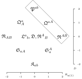
 vs  

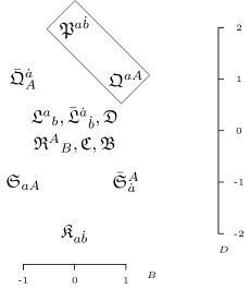
Figure 3: The symmetry generators of $\mathfrak{osp}(6|4)$ (lhs) and $\mathfrak{psu}(2,2|4)$ (rhs). In $\mathfrak{psu}(2,2|4)$ the generators can be arranged according to their hyper- and dilatation charge. Similarly, we can arrange the generators of $\mathfrak{osp}(6|4)$ if we replace the hypercharge by a $\mathfrak{u}(1)$ R-symmetry charge. In $\mathcal{N}=4$ SYM theory, the dual or level-one Yangian generators $\mathfrak{P}^{(1)}$ and $\mathfrak{Q}^{(1)}$ were identified with the generators $\mathfrak{S}^{(0)}$ and $\mathfrak{K}^{(0)}$, respectively. The picture on the left suggests a similar dualization for $\mathcal{N}=6$ SCS theory incorporating the R-symmetry.

In [37], this relation of different $\mathcal{N}=4$ SYM scattering amplitudes in the collinear limit was implemented into the representation of the $\mathfrak{psu}(2,2|4)$ symmetry on the scattering amplitudes. This implementation makes use of the so-called holomorphic anomaly [47, 48, 49], which originates in the fact that four-dimensional massless momenta factorize into complex conjugate spinors ($p_{4\mathrm{d}}=\lambda\bar{\lambda}$). In three dimensions, on the other hand, massless momenta are determined by a single real spinor ($p_{3\mathrm{d}}=\lambda\lambda$) which does not allow for a holomorphic anomaly. Hence, a straightforward generalization of the symmetry relation between amplitudes in the collinear or factorization limit to $\mathcal{N}=6$ SCS theory is not obvious. It lacks a source for a similar anomaly as in the four-dimensional case.

In $\mathcal{N}=4$ SYM theory, studying the duality between scattering amplitudes and Wilson loops revealed a dual superconformal symmetry. The presence of this extra symmetry then lead to the finding of Yangian symmetry of the scattering amplitudes. Even more, the dual symmetry was identified with the level-one Yangian generators [36]. Though in $\mathcal{N}=6$ SCS theory a similar extra symmetry is not known, there is a straightforward way to construct level-one generators from the local $\mathfrak{osp}(6|4)$ symmetry yielding a Yangian algebra. We showed that the four- and six-point tree-level amplitudes of $\mathcal{N}=6$ SCS theory are indeed invariant under this Yangian algebra, and that the Yangian generators obey the Serre relations, which ensures that the Yangian algebra is consistent.

The fact that $\mathcal{N}=6$ SCS theory in the planar limit gains extra symmetries in the form of integrability seems to be related to special properties of the underlying symmetry algebra $\mathfrak{osp}(6|4)$, namely the vanishing of the quadratic Casimir in the adjoint representation (see also [61, 62]). It is interesting to notice that, while in the four-dimensional case the algebra with this special property is the maximal superconformal algebra $\mathfrak{psu}(2,2|4)$, in three dimensions it is not the maximal superconformal algebra $\mathfrak{osp}(8|4)$, but $\mathfrak{osp}(6|4)$ that has this special property.

Our findings point towards further investigations. Among others, one should consider the AdS/CFT dual of $\mathcal{N}=6$ SCS theory, since in $\mathcal{N}=4$ SYM theory the comparison with results from $\mathrm{AdS}_{5}\times\mathrm{S}^{5}$ strings has been extremely useful. The dual superconformal symmetry of scattering amplitudes in $\mathcal{N}=4$ SYM theory can be traced back to a T-self-duality of the $\mathrm{AdS}_{5}\times\mathrm{S}^{5}$ background of the dual string theory [32, 33]. Such a duality seems not to be admitted by $\mathrm{AdS}_{4}\times\mathbb{C}\mathrm{P}^{3}$, the string theory background corresponding to $\mathcal{N}=6$ SCS theory [44]. Can this problem be reconsidered?

In their search for a T-dualization, the authors of [44] assume that the dualization does not involve the $\mathbb{C}\mathrm{P}^{3}$ coordinates. On the other hand, the structure of the $\mathfrak{osp}(6|4)$ algebra seems to call for a T-dualization of $3+3$ bosonic and $6$ fermionic coordinates dual to the generators $\left\{\mathfrak{P}^{ab},\mathfrak{R}^{AB},\mathfrak{Q}^{aA}\right\}$ (cf. Figure 3). The contributions to the dilaton shift coming from bosonic and fermionic dualization seem to cancel out. However, this formal T-duality is not compatible with the reality conditions of the coordinates; still it seems worthwhile to investigate it further. The problem with T-dualizing the coordinates of $\mathbb{C}\mathrm{P}^{3}$ appears to be connected to the lack of a definition of $\delta(R)$ in our setup.

Other hints for rephrasing the Yangian symmetry in terms of some dual symmetry could come form perturbative computations in $\mathcal{N}=6$ SCS. In particular, the IR divergences for scattering amplitudes could possibly be mapped to the UV divergences of some other object (maybe a Wilson loop in higher dimensions). Any results in this direction might also shed light on the duality between non-MHV amplitudes and Wilson loops in $\mathcal{N}=4$ SYM theory, since the amplitudes in $\mathcal{N}=6$ SCS theory are very similar to those. A starting point for the investigation of Wilson loops in $\mathcal{N}=6$ SCS was set in the very recent work [63].

There are many more open questions and directions for further study. They comprise the extension of our results to higher point amplitudes, their extension to loop-level and in particular the understanding of corresponding quantities in the AdS/CFT dual of the three-dimensional gauge theory. One of the most interesting problems seems to be whether one can find a systematic way to determine (tree-level) scattering amplitudes in $\mathcal{N}=6$ SCS theory. An apparent ansatz would be an adaption of the BCFW recursion relations [64, 65] of $\mathcal{N}=4$ SYM theory. This problem is currently under investigation.

Recently, a remarkable generating functional for $\mathcal{N}=4$ SYM scattering amplitudes was proposed [66]. The functional takes the form of a Graßmannian integral that reproduces different contributions to scattering amplitudes. These contributions have been shown to be (cyclic by construction) Yangian invariants [67, 68, 69, 70]. It would be interesting to investigate whether an analogous formula exists for the three-dimensional case studied in this paper. The (S)Clifford realization presented in Appendix A could play a similar role for $\mathfrak{osp}(2k+2|2k)$ as the twistorial realizations plays in the case of $\mathfrak{psu}(m|m)$.

Acknowledgments.

We would like to thank Niklas Beisert, Tristan McLoughlin and Matthias Staudacher for many helpful discussions, suggestions as well as comments on the manuscript. In particular, we are grateful to Tristan McLoughlin for his initial collaboration on this project. We further thank Lucy Gow, Yu-tin Huang, Jakob Palmkvist and Soo-Jong Rey for discussions on various related topics.

Appendix A From (S)Clifford algebra to Spinor/Metaplectic representations

In this appendix we want to stress that the singleton representation of $\mathfrak{osp}(6|4)$ we are using in this paper (see Section 4) is nothing but the natural generalization of the familiar spinor representation of $\mathfrak{so}(2k)$. Moreover we will emphasize some special properties of this realization that makes the Yangian generators defined in Section 7 satisfy the Serre relations (7.2).

Let us first review the familiar $\mathfrak{so}(2k)$ case. It is well-known that if one has a representation of the Clifford algebra:

$$\left\{\gamma^{i},\gamma^{j}\right\}=g^{ij}\,,$$ (A.1)

for a given symmetric form $g^{ij}$, where $i,j=1,\dots 2k$, then the objects

$$T^{ij}\sim\left[\gamma^{i},\gamma^{j}\right]\,,$$ (A.2)

satisfy the $\mathfrak{so}(2k)$ algebra commutation relations

$$\left[T^{ij},T^{kl}\right]\sim g^{jk}T^{il}+\dots$$ (A.3)

where the dots mean: Add three more terms such that the symmetry properties of the indices are the same as on the right hand side. The realization (A.2) still does not look like the R-symmetry generators in (4.12). To obtain (4.12) from (A.2) one has to choose an embedding of $\mathfrak{u}(k)$ into $\mathfrak{so}(2k)$ and define creation/annihilation type fermionic variables

$$\eta^{A}\equiv\mathcal{A}^{+A}_{j}\gamma^{j}\,,\qquad\qquad\frac{\partial}{\partial\eta^{A}}\equiv\mathcal{A}^{-}_{Aj}\gamma^{j}\,,$$ (A.4)

where $A=1,\dots k$ is a $\mathfrak{u}(k)$ index and $\mathcal{A}^{+A}_{j},\mathcal{A}^{-}_{Aj}$ have to satisfy

$$\mathcal{A}^{+A}_{i}g^{ij}\mathcal{A}^{-}_{Bj}=\delta^{A}_{B}\,,\qquad\qquad\mathcal{A}^{+A}_{i}g^{ij}\mathcal{A}^{+B}_{j}=0\,,\qquad\qquad\mathcal{A}^{-}_{Ai}g^{ij}\mathcal{A}^{-}_{Bj}=0,$$ (A.5)

in order that $\eta^{A},\frac{\partial}{\partial\eta^{A}}$ satisfy canonical anticommutation relations. More explicitly, the R-symmetry generators in (4.12) are related to the ones in (A.2) via

$$\mathfrak{R}^{AB}\sim\mathcal{A}^{+A}_{i}\mathcal{A}^{+B}_{j}T^{ij}\,,\qquad\qquad\mathfrak{R}^{A}_{B}\sim\mathcal{A}^{+A}_{i}\mathcal{A}^{-}_{Bj}T^{ij},\qquad\qquad\mathfrak{R}_{AB}\sim\mathcal{A}^{-}_{Ai}\mathcal{A}^{-}_{Bj}T^{ij}\,.$$ (A.6)

The realization one obtains in this way is not irreducible, but splits into two irreducible representations (with opposite chirality). Indeed, the full space of functions (necessarily polynomials) of the variables $\eta^{A}$ splits into two spaces: one made of polynomials with only even powers of $\eta^{A}$, the other with only odd powers of $\eta^{A}$. None of the generators in (4.12) connects the two.

This construction works in the very same way for $\mathfrak{sp}(2\ell)$, the main difference is that in this case the representation one obtains is infinite-dimensional. This representation is the direct analog of the spinor representation and is usually called metaplectic representation. If one starts with a representation of the algebra:

$$\left[\xi^{i},\xi^{j}\right]=\Omega^{ij}$$ (A.7)

for a given anti-symmetric (non-degenerate) form $\Omega^{ij}$, then the objects

$$S^{ij}\sim\left\{\xi^{i},\xi^{j}\right\}$$ (A.8)

satisfy the $\mathfrak{sp}(2\ell)$ algebra commutation relations

$$\left[S^{ij},S^{kl}\right]\sim\Omega^{jk}S^{il}+\dots$$ (A.9)

where again the dots mean: Add three more terms such that the symmetry properties of the indices are the same as on the right hand side. As before, one has to choose an embedding of $\mathfrak{u}(\ell)$ into $\mathfrak{sp}(2\ell)$ and define creation/annihilation type bosonic variables

$$\lambda^{a}\equiv\mathcal{B}^{+a}_{j}\xi^{j}\,,\qquad\qquad\frac{\partial}{\partial\lambda^{a}}\equiv\mathcal{B}^{-}_{aj}\xi^{j}\,,$$ (A.10)

where $a=1,\dots k$ is a $\mathfrak{u}(\ell)$ index and $\mathcal{B}^{+a}_{j},\mathcal{B}^{-}_{aj}$ have to satisfy

$$\mathcal{B}^{+a}_{i}\Omega^{ij}\mathcal{B}^{-}_{bj}=\delta^{b}_{a}\,,\qquad\qquad\mathcal{B}^{+a}_{i}\Omega^{ij}\mathcal{B}^{+b}_{j}=0\,,\qquad\qquad\mathcal{B}^{-}_{ai}\Omega^{ij}\mathcal{B}^{-}_{bj}=0$$ (A.11)

in order that $\lambda^{a},\frac{\partial}{\partial\lambda^{a}}$ satisfy canonical commutation relations. More explicitly, the bosonic generators in (4.12,7.5) are related to the ones in (A.8) via

$$\mathfrak{P}^{ab}\sim\mathcal{B}^{+a}_{i}\mathcal{B}^{+b}_{j}S^{ij}\,,\qquad\qquad\mathfrak{Y}^{a}_{b}\sim\mathcal{B}^{+a}_{i}\mathcal{B}^{-}_{bj}S^{ij},\qquad\qquad\mathfrak{K}_{ab}\sim\mathcal{B}^{-}_{ai}\mathcal{B}^{-}_{bj}S^{ij}\,.$$ (A.12)

Let us stress that at the group level spinor and metaplectic representations are representations of $\mathrm{Spin}(2k)$, $\mathrm{Mt}(2\ell)$, respectively, which are the double covers of $\mathrm{SO}(2k)$, $\mathrm{Sp}(2\ell)$.

All this easily generalizes to $\mathfrak{osp}(2k|2\ell)$ algebras. If one starts with objects satisfying

$$\left[\mathnormal{\Theta}^{\mathcal{A}},\mathnormal{\Theta}^{\mathcal{B}}\right\}=\mathcal{G}^{\mathcal{A}\mathcal{B}}\,,$$ (A.13)

where $\mathcal{A},\mathcal{B}$ label the $2k+2\ell$-dimensional fundamental representation of $\mathfrak{osp}(2k|2\ell)$, then

$$J^{\mathcal{A}\mathcal{B}}\sim\left\{\mathnormal{\Theta}^{\mathcal{A}},\mathnormal{\Theta}^{\mathcal{B}}\right]\,,$$ (A.14)

satisfy $\mathfrak{osp}(2k|2\ell)$ algebra commutation relations. After choosing an embedding of $\mathfrak{u}(k|\ell)$ into $\mathfrak{osp}(2k|2\ell)$, one obtains oscillator type realizations, like the one in (4.12).

Appendix B $\mathfrak{so}(6)$ Invariants

In this appendix we will study the problem of determining invariants under the following realization of $\mathfrak{so}(6)$:

$$\mathfrak{R}^{AB}=\sum_{J=1}^{p}\alpha_{J}^{[A}\beta_{J}^{B]}\,,$$ (B.1)

$$\mathfrak{R}_{AB}=\sum_{J=1}^{p}\frac{\partial}{\partial\alpha_{J}^{[A}}\frac{\partial}{\partial\beta_{J}^{B]}}\,,$$ (B.2)

$$\mathfrak{R}^{A}_{B}=\sum_{J=1}^{p}\left(\alpha_{J}^{A}\frac{\partial}{\partial\alpha_{J}^{B}}-\frac{\partial}{\partial\beta_{J}^{B}}\beta_{J}^{A}\right)\,,$$ (B.3)

where $\alpha_{I}^{A},\beta_{I}^{A}$ are anticommuting fermionic variables and $A,B$ are $SU(3)$ indices. $p$ is some integer, it is related to the number $n$ of amplitude legs as $2p=n-4$. This realization is completely equivalent to the following one:

$$\mathfrak{R}^{AB}=\sum_{\bar{\iota}=1}^{2p}\rho_{\bar{\iota}}^{A}\rho_{\bar{\iota}}^{B}\,,$$ (B.4)

$$\mathfrak{R}_{AB}=\sum_{\bar{\iota}=1}^{2p}\frac{\partial}{\partial\rho_{\bar{\iota}}^{A}}\frac{\partial}{\partial\rho_{\bar{\iota}}^{B}}\,,$$ (B.5)

$$\mathfrak{R}^{A}{}_{B}=\sum_{\bar{\iota}=1}^{2p}\frac{1}{2}\left(\rho_{\bar{\iota}}^{A}\frac{\partial}{\partial\rho_{\bar{\iota}}^{B}}-\frac{\partial}{\partial\rho_{\bar{\iota}}^{B}}\rho_{\bar{\iota}}^{A}\right)\,,$$ (B.6)

where $\rho_{\bar{\iota}}$ are linearly related to $\alpha^{A}_{I},\beta^{A}_{I}$, the map between $\rho$ and $\alpha,\beta$ is parametrized by a $\mathrm{O}(2p)$ freedom. Notice that this last realization makes sense also for odd $2p$.

All the generators written above are invariant under $\mathrm{O}(2p)$ rotations among the family indices. In the following we will refer to this group as dual. $\mathrm{O}(2p)_{\text{dual}}$ rotation symmetry is manifest in the form of the generators written in terms of $\rho_{\bar{\iota}}^{A}$ as a rotation of the indices $\bar{\iota}$. On the generators written in terms of $\alpha,\beta$ $\mathrm{O}(2p)_{\text{dual}}$ acts in the following way

$$\alpha_{I} \rightarrow\mathnormal{\Xi}_{I}^{J}\alpha_{J}\,, \beta^{I} \rightarrow\left(\mathnormal{\Xi}^{-1}\right)_{J}^{I}\beta^{J}\,, U(p)\,,\qquad p^{2}\quad\text{d.o.f.}$$

$$\alpha_{I} \rightarrow\alpha_{I}+\Omega_{IJ+}\beta^{J}\,, \beta^{I} \rightarrow\beta^{I}+\Omega^{IJ}_{-}\alpha_{J}\,, \frac{SO(2p)}{U(p)}\,,\qquad p(p-1)\quad\text{d.o.f.}$$

$$\alpha_{I} \rightarrow\beta^{I},, \beta^{I} \rightarrow\alpha_{I}\,, \mathbb{Z}_{2}\sim\frac{O(2p)}{SO(2p)}\,,$$ (B.7)

where $\Omega_{\pm}^{IJ}=-\Omega_{\pm}^{JI}$. The $\mathbb{Z}_{2}$ is the conjugation of $\mathfrak{su}(p)$ (outer automorphism). Notice that we raised the family index of $\beta$, we have to do this in order to interpret the family index as a $\mathfrak{u}(p)$ index.

In the following, we will show how the $\mathfrak{so}(6)$ invariants can be obtained and classified. Since the description in terms of $\alpha,\beta$ is equivalent (for integer $p$) to the one in terms of $\rho$, we will switch between the two depending on convenience.

It is instructive to first study the case $2p=1$. This case obviously makes sense only in the $\rho$ realization. In this case the full fermionic Fock space is $2^{3}=8$-dimensional and split into $4\oplus\bar{4}$ representations of $\mathfrak{so}(6)$. The two correspond to even or odd functions (just polynomials up to degree $3$) in $\rho$, respectively.

Let us now consider the next case: $p=1$. The study of this case is particularly transparent in terms of $\alpha,\beta$. To classify the states it is useful to introduce an extra operator $g$

$$g=\alpha^{A}\frac{\partial}{\partial\alpha^{A}}-\beta^{A}\frac{\partial}{\partial\beta^{A}}\,.$$ (B.8)

This operator is central with respect to $\mathfrak{so}(6)$ and is nothing but the generator of the previously mentioned dual $\mathfrak{so}(2p)|_{p=1}\sim\mathfrak{u}(1)$. In this case the full Fock space is $2^{6}=64$ dimensional, it decomposes into irreducible representations of $\mathfrak{so}(6)$ as

$$\left(4\oplus\bar{4}\right)^{2}=1_{3}\oplus 6_{2}\oplus 15_{1}\oplus 10_{0}\oplus\bar{10}_{0}\oplus 15_{-1}\,,\oplus 6_{-2}\oplus 1_{-3}$$ (B.9)

where the subscript refers to the charge under $g$ (B.8). This decomposition is concretely realized by the solutions to the equation

$$\mathfrak{R}_{AB}|\text{State}\rangle=\frac{\partial}{\partial\alpha^{[A}}\frac{\partial}{\partial\beta^{B]}}|\text{State}\rangle=0\,.$$ (B.10)

We can be more explicit and show how these states look like in the space of Graßmann variables $\alpha^{A},\beta^{A}$. For clarity we also explicitly write down the decomposition under $SO(6)\rightarrow SU(3)$.

• $1_{3}\rightarrow 1:\quad\epsilon_{ABC}\alpha^{A}\alpha^{B}\alpha^{C}$,

• $6_{2}\rightarrow\bar{3}\oplus 3:\quad\epsilon_{ABC}\alpha^{B}\alpha^{C}+\text{descendants}$,

• $15_{1}\rightarrow 3\oplus 8\oplus 1\oplus\bar{3}:\quad\alpha^{A}+\text{descendants}$,

• $10_{0}\rightarrow 1\oplus 3\oplus 6:\quad 1+\text{descendants}$,

• $\bar{10}_{0}\rightarrow\bar{6}\oplus\bar{3}\oplus 1:\quad\alpha^{(A}\beta^{B)}+\text{descendants}$,

• $15_{1}\rightarrow 3\oplus 8\oplus 1\oplus\bar{3}:\quad\beta^{A}+\text{descendants}$,

• $6_{2}\rightarrow\bar{3}\oplus 3:\quad\epsilon_{ABC}\beta^{B}\beta^{C}+\text{descendants}$,

• $1_{3}\rightarrow 1:\quad\epsilon_{ABC}\beta^{A}\beta^{B}\beta^{C}$,

where descendants means obtained acting with $\mathfrak{R}^{AB}$.

We will now consider the case $p=2$, namely

$$\left(4\oplus\bar{4}\right)^{4}\,.$$ (B.11)

We can just take the expression (B.9) and square it. We will not write down the whole tensor product decomposition, but just list the singlets. One can easily check that there are $12$ singlets coming from $15_{\pm 1}\otimes 15_{\pm 1},6_{\pm 2}\otimes 6_{\pm 2},1_{\pm 3}\otimes 1_{\pm 3}$, where the signs have to be considered independently; and two further singlets are contained in $10_{0}\otimes\bar{10}_{0}$ ($2$ times). For convenience we will list the explicit expressions of the singlets:

• $15_{\pm 1}\otimes 15_{\pm 1}$ contains 4 singlets:

  $$\epsilon_{ABG}\epsilon_{EFC}\alpha_{1}^{A}\alpha_{1}^{(B}\beta_{1}^{C)}\alpha_{2}^{E}\alpha_{2}^{(F}\beta_{2}^{G)},\qquad(\alpha_{1}\leftrightarrow\beta_{1})\text{ and/or }(\alpha_{2}\leftrightarrow\beta_{2}).$$ (B.12)

• $6_{\pm 2}\otimes 6_{\pm 2}$ contains 4 singlets:

  $$\epsilon_{ABC}\epsilon^{ADE}\alpha_{1}^{B}\alpha_{1}^{C}\epsilon_{DFG}\alpha_{2}^{F}\alpha_{2}^{G}\epsilon_{EHI}\beta_{2}^{H}\beta_{2}^{I},\qquad(\alpha\leftrightarrow\beta)\text{ and/or }(1\leftrightarrow 2).$$ (B.13)

• $1_{\pm 3}\otimes 1_{\pm 3}$ contains 4 singlets:

  $$\epsilon_{ABC}\alpha_{1}^{A}\alpha_{1}^{B}\alpha_{1}^{C}\epsilon_{DEF}\alpha_{2}^{D}\alpha_{2}^{E}\alpha_{2}^{F},\qquad(\alpha_{1}\leftrightarrow\beta_{1})\text{ and/or }(\alpha_{2}\leftrightarrow\beta_{2}).$$ (B.14)

• $10_{0}\otimes\bar{10}_{0}$ contains $2$ singlets:

  $$\epsilon_{ACD}\epsilon_{BEF}\alpha_{1}^{A}\beta_{1}^{B}\alpha_{2}^{C}\alpha_{2}^{D}\beta_{2}^{E}\beta_{2}^{F},\qquad(1\leftrightarrow 2).$$ (B.15)

A question one can ask is how these singlets transform among themselves under the $\mathfrak{so}(2p)|_{p=2}=\mathfrak{so}(4)_{\mathrm{dual}}$ transformations. This question can be answered noticing that the quantities

$$g_{I}=\alpha^{A}_{I}\frac{\partial}{\partial\alpha^{A}_{I}}-\beta^{A}_{I}\frac{\partial}{\partial\beta^{A}_{I}}\,.$$ (B.16)

(no sum over $I$), are nothing but the Cartan generators of the $\mathfrak{so}(4)_{\mathrm{dual}}$, and these singlets are indeed labeled by $(g_{1},g_{2})$.

The $\mathfrak{so}(4)_{\mathrm{dual}}$ transformation properties of the singlets can also be obtained considering where the singlets come from in

$$\left(4\oplus\bar{4}\right)^{4}\,.$$ (B.17)

The $\mathfrak{so}(4)_{\mathrm{dual}}$ acts as a rotation of the four factors $(4\oplus\bar{4})$ in the fourfold tensor product above. Keeping in mind that a tensor product of $n_{4}$ fundamental with $n_{\bar{4}}$ antifundamental can contain singlets only if $n_{4}-n_{\bar{4}}=0(\mathrm{mod}\>4)$, it is easy to see that singlets can only come from

• $4\otimes 4\otimes 4\otimes 4$: $1$ singlet under $\mathfrak{so}(6)_{\mathfrak{R}}$, singlet also under $\mathfrak{so}(4)_{\text{dual}}$,

• $\bar{4}\otimes\bar{4}\otimes\bar{4}\otimes\bar{4}$: 1 singlet under $\mathfrak{so}(6)_{\mathfrak{R}}$, singlet also under $\mathfrak{so}(4)_{\text{dual}}$,

• $\bar{4}\otimes\bar{4}\otimes 4\otimes 4$: $2$ singlets under $\mathfrak{so}(6)_{\mathfrak{R}}$ $\times$ $\mathbf{\underline{6}}$ under $\mathfrak{so}(4)_{\text{dual}}$,

in the last line the combinatorial factor $\binom{4}{2}=\mathbf{\underline{6}}$ corresponding to the possible ways of choosing two $4$ and two $\bar{4}$ in (B.17), is also the dimension of the $\mathfrak{so}(4)_{\text{dual}}$ representation under which these ($\mathfrak{so}(6)_{\mathfrak{R}}$) singlets transform.

The cases $p=3$

$$\left(4\oplus\bar{4}\right)^{6}\,,$$ (B.18)

can be considered analogously giving

• $4\otimes 4\otimes 4\otimes 4\otimes 4\otimes\bar{4}$: $4$ singlets under $\mathfrak{so}(6)_{\mathfrak{R}}$ $\times$ $\mathbf{\underline{6}}$ under $\mathfrak{so}(6)_{\text{dual}}$,

• $\bar{4}\otimes\bar{4}\otimes\bar{4}\otimes\bar{4}\otimes\bar{4}\otimes 4$: $4$ singlets under $\mathfrak{so}(6)_{\mathfrak{R}}$ $\times$ $\mathbf{\underline{6}}$ under $\mathfrak{so}(6)_{\text{dual}}$,

• $\bar{4}\otimes\bar{4}\otimes\bar{4}\otimes 4\otimes 4\otimes 4$: $6$ singlets under $\mathfrak{so}(6)_{\mathfrak{R}}$ $\times$ $\mathbf{\underline{20}}$ under $\mathfrak{so}(6)_{\text{dual}}$,

where again the combinatorial factors $\binom{6}{1}=\mathbf{\underline{6}}$, $\binom{6}{3}=\mathbf{\underline{20}}$ are also the dimensions of the $\mathfrak{so}(6)_{\text{dual}}$ representations.

The general $p>3$ cases can be studied similarly.

Appendix C Determinability of the Six-Point Superamplitude

This appendix is devoted to the study of the invertibility of equation (6.10). More precisely, we will show under which conditions one can solve (6.10) for $f_{\pm}$ in terms of the component amplitudes $A_{6\psi}$, $A_{6\phi}$. This is an important step, as the determination of the six-point superamplitude, and, thus the determination of all six-point component amplitudes relies on it. Let us define the following quantities

$$A(\pm)_{ijk}\equiv\begin{pmatrix}\lambda^{1}_{i}&\lambda^{2}_{i}&x^{\pm}_{i}\\ \lambda^{1}_{j}&\lambda^{2}_{j}&x^{\pm}_{j}\\ \lambda^{1}_{k}&\lambda^{2}_{k}&x^{\pm}_{k}\\ \end{pmatrix}\,.$$ (C.1)

$$D_{\pm}\equiv\det\left(A(\pm)_{ijk}\right)\,,\qquad\qquad\bar{D}_{\pm}\equiv\det\left(A(\pm)_{\bar{i}\bar{j}\bar{k}}\right)\,,$$ (C.2)

for some fixed $i\neq j\neq k$, and let $\left\{\bar{i},\bar{j},\bar{k}\right\}\equiv\left\{1,\ldots,6\right\}\setminus\left\{i,j,k\right\}$ as a set. Equation (6.10) can be inverted iff

$$D_{+}^{3}\bar{D}_{-}^{3}-D_{-}^{3}\bar{D}_{+}^{3}\neq 0\,.$$ (C.3)

Using $\lambda^{a}\cdot\lambda^{b}=0$, $x^{\pm}\cdot\lambda^{a}=0$, $x^{\pm}\cdot x^{\pm}=0$, $x^{+}\cdot x^{-}=1$, one can show, performing matrix multiplication, that

$$A^{T}(\pm)_{ijk}A(\pm)_{ijk}=-A^{T}(\pm)_{\bar{i}\bar{j}\bar{k}}A(\pm)_{\bar{i}\bar{j}\bar{k}}\,,$$ (C.4)

$$A^{T}(\pm)_{ijk}A(\mp)_{ijk}=-A^{T}(\pm)_{\bar{i}\bar{j}\bar{k}}A(\mp)_{\bar{i}\bar{j}\bar{k}}+\Bigl{(}\begin{smallmatrix}0&0&0\\ 0&0&0\\ 0&0&1\end{smallmatrix}\Bigr{)}\,,$$ (C.5)

where $T$ means transposition. These two equations imply respectively that

$$D_{\pm}^{2}=-\bar{D}_{\pm}^{2}\Rightarrow\bar{D}_{\pm}=is_{\pm}D_{\pm}\,,$$ (C.6)

$$D_{+}D_{-}+\bar{D}_{+}\bar{D}_{-}=\det\left((p_{i}+p_{j}+p_{k})^{ab}\right)\,,$$ (C.7)

where $s_{\pm}$ are undetermined signs. Using (C.6), (C.7) can be rewritten as

$$D_{+}D_{-}\left(1-s_{+}s_{-}\right)=\det\left((p_{i}+p_{j}+p_{k})^{ab}\right)\,.$$ (C.8)

Since for generic momentum configurations $(p_{i}+p_{j}+p_{k})^{2}$ is not vanishing, it follows that $s_{+}=s$, $s_{-}=-s$ for some sign $s$. This shows that, for generic momentum configurations, (C.3) holds, indeed

$$D_{+}^{3}\bar{D}_{-}^{3}-D_{-}^{3}\bar{D}_{+}^{3}=i(s_{+}-s_{-})D_{+}^{3}D_{-}^{3}=2isD_{+}^{3}D_{-}^{3}=\frac{is}{4}\det\left((p_{i}+p_{j}+p_{k})^{ab}\right)^{3}\neq 0\,.$$ (C.9)

To summarize, the quantities $D_{\pm}$, $\bar{D}_{\pm}$ are not independent. Given $(p_{i}+p_{j}+p_{k})^{2}$, they are determined up to a sign $s$ and a single function (which is a phase once we impose the correct reality conditions). This freedom corresponds to the $\mathrm{O}(n-4)|_{n=6}=\mathrm{O}(2)$ relevant freedom in the choice of $x^{\pm}$ mentioned in Section 5. The sign is $\mathrm{O}(2)/\mathrm{SO}(2)$, and corresponds to exchanging $x^{+}$ and $x^{-}$; the freedom that remains, $D^{\pm}\rightarrow\mathnormal{\Xi}^{\pm 1}D^{\pm}$, corresponds to the $\mathrm{SO}(2)\sim\mathrm{U}(1)$ freedom of rescaling $x^{\pm}\rightarrow\mathnormal{\Xi}^{\pm 1/3}x^{\pm}$.

Appendix D Two Component Amplitude Calculations

In the following, the amplitudes between six scalars and between six fermions are computed. As discussed in section Section 6, these two amplitudes uniquely determine the six-point superamplitude. For simplicity, consider only (anti)particles of the same flavor; set

$$\phi=\phi^{4}\,,\quad\bar{\phi}=\bar{\phi}_{4}\,,\quad\psi=\psi_{4}\,,\quad\bar{\psi}=\bar{\psi}^{4}\,.$$ (D.1)

The action of $\mathcal{N}=6$ superconformal Chern–Simons theory is $S=k/4\pi\int d^{3}x\,\mathcal{L}$. Neglecting terms that are irrelevant for the two specific amplitudes we are interested in, the Lagrangian reads (see e.g. [4, 73, 10])

$$\mathcal{L}=\mathop{\mathrm{Tr}}\Bigl{[}\varepsilon^{\mu\nu\lambda}\bigl{(}A_{\mu}\partial_{\nu}A_{\lambda}+{\textstyle\frac{2}{3}}A_{\mu}A_{\nu}A_{\lambda}-\hat{A}_{\mu}\partial_{\nu}\hat{A}_{\lambda}-{\textstyle\frac{2}{3}}\hat{A}_{\mu}\hat{A}_{\nu}\hat{A}_{\lambda}\bigr{)}-{\textstyle\frac{i}{2}}\bar{\psi}^{a}\not{D}_{ab}\psi^{b}+D_{\mu}\bar{\phi}D^{\mu}\phi\Bigr{]}\,.$$ (D.2)

The gauge fields $A_{\mu}$, $\hat{A}_{\mu}$ transform in $(\mathbf{ad},\mathbf{1})$, $(\mathbf{1},\mathbf{ad})$ representations of the gauge group. The covariant derivative $D_{\mu}$ acts on fields $\chi\in\{\phi,\psi\}$, $\bar{\chi}\in\{\bar{\phi},\bar{\psi}\}$ as

$$D_{\mu}\chi=\partial_{\mu}\chi+A_{\mu}\chi-\chi\hat{A}_{\mu}\,,\quad D_{\mu}\bar{\chi}=\partial_{\mu}\bar{\chi}+\hat{A}_{\mu}\bar{\chi}-\bar{\chi}A_{\mu}\,,\quad\not{D}_{ab}=\sigma^{\mu}_{ab}D_{\mu}\,.$$ (D.3)

The Feynman rules can be straightforwardly derived from $\mathcal{L}$, using the Faddeev–Popov regularization for the gauge field propagators.

Six-Fermion Amplitude.

The tree-level amplitude

$$\hat{A}_{6\psi}\mathrel{:=}\hat{A}_{6}(\psi_{1}{}^{A_{1}}_{\bar{A}_{1}},\bar{\psi}_{2}{}^{\bar{B}_{2}}_{B_{2}},\psi_{3}{}^{A_{3}}_{\bar{A}_{3}},\bar{\psi}_{4}{}^{\bar{B}_{4}}_{B_{4}},\psi_{5}{}^{A_{5}}_{\bar{A}_{5}},\bar{\psi}_{6}{}^{\bar{B}_{6}}_{B_{6}})\,,\quad\psi_{k}\mathrel{:=}\psi(\lambda_{k})$$ (D.4)

can be color-ordered (3.4). The color-ordered amplitude $A_{6\psi}(\lambda_{1},\ldots,\lambda_{6})$ contains all contributions in which the fields $\psi_{1},\ldots,\psi_{6}$ are cyclically connected by color contractions,

$$\hat{A}_{6\psi}=\ldots+A_{6\psi}(\lambda)\,\delta_{\bar{A}_{1}}^{\bar{B}_{2}}\delta_{B_{2}}^{A_{3}}\delta_{\bar{A}_{3}}^{\bar{B}_{4}}\delta_{B_{4}}^{A_{5}}\delta_{\bar{A}_{5}}^{\bar{B}_{6}}\delta_{B_{6}}^{A_{1}}+\ldots\,,\quad\lambda\mathrel{:=}(\lambda_{1},\ldots,\lambda_{6})\,.$$ (D.5)

Two kinematically different diagrams contribute to $A_{6\psi}(\lambda)$, see Figures 4,5.

Figure 4: Diagram A, which contributes to the six-fermion amplitude. Blue/dashed lines represent fundamental color contractions, red/solid lines represent antifundamental ones. When color-stripped, the left diagram gives (D.6), and the right diagram equals the left one up to a relabeling of the external legs.

Figure 5: Diagram B, which contributes to the six-fermion amplitude. When color-stripped, the left diagram gives (D.8), and the other two diagrams equal the left one up to relabelings of the external legs.

Diagram A (left in Figure 4) evaluates to

$$A_{6\psi,\mathrm{A}}(1,\ldots,6)=\frac{C_{6}}{3}\frac{1}{\langle 12\rangle\langle 34\rangle\langle 56\rangle^{2}}\cdot\\ \cdot\Bigl{[}\bigl{(}\langle 1|p_{56}|1\rangle-\langle 2|p_{56}|2\rangle\bigr{)}\bigl{(}\langle 5|p_{3}|6\rangle-\langle 5|p_{4}|6\rangle\bigr{)}-\bigl{\{}(1,2)\leftrightarrow(3,4)\bigr{\}}\Bigr{]}\,,$$ (D.6)

where $A(k_{1},\ldots,k_{6}):=A(\lambda_{k_{1}},\ldots,\lambda_{k_{6}})$, and for any momenta $q_{1},\ldots,q_{k}$

$$\langle i|q_{1}|\ldots|q_{k}|j\rangle\mathrel{:=}\lambda_{i}^{a}\varepsilon_{ab}q_{1}^{bc}\varepsilon_{cd}\cdots\varepsilon_{ef}q_{k}^{fg}\varepsilon_{gh}\lambda_{j}^{h}\,.$$ (D.7)

The overall constant $C_{6}$ shall be left undetermined. Diagram B (left in Figure 5) reads

$$A_{6\psi,\mathrm{B}}(1,\ldots,6)=2C_{6}\biggl{[}\frac{\langle 13\rangle\langle 64\rangle\langle 1|p_{23}|4\rangle}{\langle 12\rangle\langle 45\rangle p_{123}^{2}}+\{1\leftrightarrow 2\}+\{4\leftrightarrow 5\}+\{1\leftrightarrow 2,4\leftrightarrow 5\}\biggr{]}\,.$$ (D.8)

The total color-ordered amplitude is a sum over all relabelings of the diagrams in Figures 4,5 that respect the color structure (D.5). The result is

$$A_{6\psi}(1,\ldots,6)= +A_{6\psi,\mathrm{A}}(1,2,3,4,5,6)+A_{6\psi,\mathrm{A}}(1,6,5,4,3,2)$$

$$+A_{6\psi,\mathrm{B}}(1,2,3,4,5,6)-A_{6\psi,\mathrm{B}}(6,5,4,3,2,1)$$

$$+A_{6\psi,\mathrm{B}}(1,2,3,6,5,4)+A_{6\psi,\mathrm{B}}(3,2,1,4,5,6)+\{\text{two cyclic}\}\,.$$ (D.9)

Here, “two cyclic” stands for two repetitions of all previous terms with the relabelings $\lambda_{k}\to\lambda_{k+2}$, $\lambda_{k}\to\lambda_{k+4}$ $(\mathrm{mod}\>6)$ applied. Using Schouten’s identity and various relations following from momentum conservation ($P=0$), this can be simplified to

$$A_{6\psi}(1,\ldots,6)=C_{6}\cdot\\ \cdot\biggl{(}\!\!\Bigl{(}\frac{-{\textstyle\frac{1}{3}}\langle 1|p_{3}|p_{5}|1\rangle+{\textstyle\frac{1}{3}}\langle 2|p_{4}|p_{6}|2\rangle-\langle 3|p_{2}|p_{5,-6}|3\rangle}{\langle 12\rangle\langle 34\rangle\langle 56\rangle}-2\frac{\langle 2|p_{3,-4}|p_{234}|p_{5,-6}|1\rangle}{\langle 34\rangle\langle 56\rangle p_{234}^{2}}-\{\text{shift by one}\}\!\Bigr{)}\\ -2\frac{\langle 1|p_{6}|p_{6,-1,2}|p_{345}|p_{3,-4,5}|p_{3}|4\rangle+\langle 1|p_{2}|p_{6,-1,2}|p_{345}|p_{3,-4,5}|p_{5}|4\rangle}{\langle 6|p_{1}|2\rangle\langle 3|p_{4}|5\rangle p_{612}^{2}}\biggr{)}+\{\text{two cyclic}\}\,,$$ (D.10)

where “shift by one” means the relabeling $\lambda_{k}\to\lambda_{k+1}\,(\mathrm{mod}\>6)$.

Six-Scalar Amplitude.

Again the color-ordered amplitude $A_{6\phi}(\lambda_{1},\ldots,\lambda_{6})$ contains all contributions in which the fields $\phi_{1},\ldots,\phi_{6}$ are cyclically connected by color contractions,

$$\hat{A}_{6\phi}\mathrel{:=}{} \hat{A}_{6}(\phi_{1}{}^{A_{1}}_{\bar{A}_{1}},\bar{\phi}_{2}{}^{\bar{B}_{2}}_{B_{2}},\phi_{3}{}^{A_{3}}_{\bar{A}_{3}},\bar{\phi}_{4}{}^{\bar{B}_{4}}_{B_{4}},\phi_{5}{}^{A_{5}}_{\bar{A}_{5}},\bar{\phi}_{6}{}^{\bar{B}_{6}}_{B_{6}}) \phi_{k} \mathrel{:=}\phi(\lambda_{k})$$

$$={} \ldots+A_{6\phi}(\lambda)\,\delta_{\bar{A}_{1}}^{\bar{B}_{2}}\delta_{B_{2}}^{A_{3}}\delta_{\bar{A}_{3}}^{\bar{B}_{4}}\delta_{B_{4}}^{A_{5}}\delta_{\bar{A}_{5}}^{\bar{B}_{6}}\delta_{B_{6}}^{A_{1}}+\ldots\,, \lambda \mathrel{:=}(\lambda_{1},\ldots,\lambda_{6})\,.$$ (D.11)

The color-ordered amplitude receives contributions from three kinematically different diagrams. Two of them are the diagrams A and B, Figures 4,5, with all fermion lines replaced by scalar lines. The scalar version of diagram A (left in Figure 4) reads

$$A_{6\phi,\mathrm{A}}(1,\ldots,6)=-\frac{4C_{6}}{3}\frac{1}{\langle 12\rangle\langle 34\rangle\langle 56\rangle^{2}}\Bigl{(}\langle 1|p_{6}|2\rangle\langle 3|p_{5}|4\rangle-\{5\leftrightarrow 6\}\Bigr{)}\,,$$ (D.12)

while the scalar version of diagram B (left in Figure 5) is

$$A_{6\phi,\mathrm{B}}(1,\ldots,6)=8C_{6}\frac{\langle 1|p_{3}|2\rangle\langle 4|p_{6}|5\rangle}{\langle 12\rangle\langle 45\rangle p_{123}^{2}}\,.$$ (D.13)

A further contribution comes from diagram C, see Figure 6.

Figure 6: Diagram C that contributes to the six-scalar amplitude. Again, blue/dashed lines represent fundamental color contractions, red/solid lines represent antifundamental ones. When color-stripped, the left diagram gives (D.14), and the other two diagrams equal the left one up to relabelings of the external legs.

It evaluates to

$$A_{6\phi,\mathrm{C}}(1,\ldots,6)=-2C_{6}\frac{\langle 16\rangle\langle 25\rangle+\langle 15\rangle\langle 26\rangle}{\langle 12\rangle\langle 56\rangle}\,.$$ (D.14)

Again, the total color-ordered amplitude is a sum over all relabelings of these diagrams that respect the color structure. The sum of all contributions is

$$A_{6\phi}(1,\ldots,6)= +A_{6\phi,\mathrm{A}}(1,2,3,4,5,6)+A_{6\phi,\mathrm{A}}(1,6,5,4,3,2)$$

$$+A_{6\phi,\mathrm{B}}(1,2,3,4,5,6)+A_{6\phi,\mathrm{B}}(6,5,4,3,2,1)$$

$$-A_{6\phi,\mathrm{B}}(1,2,3,6,5,4)-A_{6\phi,\mathrm{B}}(3,2,1,4,5,6)$$

$$+A_{6\phi,\mathrm{C}}(1,2,3,4,5,6)+A_{6\phi,\mathrm{C}}(3,2,1,6,5,4)$$

$$-2A_{6\phi,\mathrm{C}}(1,2,3,6,5,4)+\{\text{two cyclic}\}\,.$$ (D.15)

This can be simplified to

$$A_{6\phi}(1,\ldots,6)=C_{6}\biggl{(}4\frac{\langle 3|p_{5}|p_{1}|p_{6}|p_{2}|p_{4}|3\rangle+\langle 14\rangle^{2}\langle 2|p_{3}|p_{6}|p_{5}|2\rangle}{\langle 1|p_{2}|p_{3}|p_{4}|p_{5}|p_{6}|1\rangle}\\ +\Bigl{(}2\frac{{\textstyle\frac{1}{3}}\langle 16\rangle\langle 35\rangle\langle 24\rangle-{\textstyle\frac{1}{3}}\langle 13\rangle\langle 56\rangle\langle 24\rangle+\langle 16\rangle\langle 23\rangle\langle 45\rangle}{\langle 12\rangle\langle 34\rangle\langle 56\rangle}+8\frac{\langle 5|p_{1}|6\rangle\langle 3|p_{2}|4\rangle}{\langle 34\rangle\langle 56\rangle p_{234}^{2}}+\{\text{shift by one}\}\Bigr{)}\\ -8\frac{\langle 26\rangle\langle 35\rangle(\langle 16\rangle^{2}\langle 34\rangle^{2}+\langle 12\rangle^{2}\langle 45\rangle^{2})}{\langle 2|p_{1}|6\rangle\langle 3|p_{4}|5\rangle p_{612}^{2}}\biggr{)}+\{\text{two cyclic}\}\,.$$ (D.16)

Appendix E Factorization of the Six-Point Superamplitude

Consider the quantity:

$$\int d^{2|3}\hat{\mathnormal{\Lambda}}\,\mathcal{A}_{4}(\mathnormal{\Lambda}_{1},\mathnormal{\Lambda}_{2},\mathnormal{\Lambda}_{3},\hat{\mathnormal{\Lambda}})\frac{1}{P_{13}^{2}}\mathcal{A}_{4}(\pm i\hat{\mathnormal{\Lambda}},\mathnormal{\Lambda}_{4},\mathnormal{\Lambda}_{5},\mathnormal{\Lambda}_{6})\,,$$ (E.1)

where $\mathnormal{\Lambda}=(\lambda^{a},\eta^{A})$ and the result doesn’t depend on the choice of sign $\pm$ . The integration can be trivially performed because of the delta functions using:

$$\int d^{3}\hat{\eta}\,\delta^{6}(Q_{1}^{Aa}+\hat{\eta}^{A}\mu^{a})\,\delta^{6}(Q_{2}^{Aa}-\hat{\eta}^{A}\mu^{a})=\delta^{6}(Q_{1}^{Aa}+Q_{2}^{Aa})\,\delta^{3}(\epsilon_{ab}Q_{1}^{Aa}\mu^{b})$$ (E.2)

and

$$\int d^{2}\hat{\lambda}\,\delta^{3}(P_{1}^{ab}+\hat{\lambda}^{a}\hat{\lambda}^{b})\,\delta^{3}(P_{2}^{ab}-\hat{\lambda}^{a}\hat{\lambda}^{b})F(\hat{\lambda})=\delta^{3}(P_{1}^{ab}+P_{2}^{ab})\,\delta(P_{1}^{2})\left(F(\hat{\lambda})+F(-\hat{\lambda})\right)$$ (E.3)

where on the right hand side $\hat{\lambda}$ is the solution to the equation $\hat{\lambda}^{a}\hat{\lambda}^{b}=P_{2}^{ab}$. Reminding that (6.2)

$$\mathcal{A}_{4}(1,2,3,4)=\delta^{3}(P)\,\delta^{6}(Q)f(\lambda_{1},\lambda_{2},\lambda_{3},\lambda_{4})\,,$$ (E.4)

and using the properties of $f(\lambda)$, we obtain:

$$\frac{1}{P_{13}^{2}}\delta(P_{13}^{2})\,\delta^{3}(P)\,\delta^{3}(Q)\,\delta^{3}({\epsilon_{ab}Q_{13}^{Aa}\hat{\lambda}^{b}})f(\lambda_{1},\lambda_{2},\lambda_{3},\hat{\lambda})f(\pm i\hat{\lambda},\lambda_{4},\lambda_{5},\lambda_{6})\,.$$ (E.5)

This can be rewritten as

$$\frac{1}{P_{13}^{2}}\delta(P_{13}^{2})\,\delta^{3}(P)\,\delta^{6}(Q)\delta^{3}(\alpha)f^{+}(\lambda)\,,$$ (E.6)

which equals $\mathcal{A}_{6}$ in the limit $P_{13}^{2}\to 0$, cf. Section 6.

Appendix F The Metric of $\mathfrak{osp}(6|4)$

Introducing matrices $(E^{\mathbb{A}}{}_{\mathbb{B}})^{i}{}_{j}=\delta^{\mathbb{A}i}\delta_{\mathbb{B}j}$ with $\mathbb{A},\mathbb{B}=a,b,A,B,\dots$, the fundamental representation $M$ of $\mathfrak{osp}(6|4)$ consisting of $(4|6)\times(4|6)$ matrices can be written as

$$M\left[\left(\begin{array}[]{cc|cc}\mathfrak{L}^{a}{}_{b}&\mathfrak{P}^{ab}&\mathfrak{Q}^{a}{}_{A}&\mathfrak{Q}^{aA}\\ \mathfrak{K}_{ab}&\mathfrak{L}^{a}{}_{b}&\mathfrak{S}_{aA}&\mathfrak{S}_{a}{}^{A}\\ \hline\cr\mathfrak{S}_{a}{}^{A}&\mathfrak{Q}^{aA}&\mathfrak{R}^{A}{}_{B}&\mathfrak{R}^{AB}\\ \mathfrak{S}_{aA}&\mathfrak{Q}^{a}{}_{A}&\mathfrak{R}_{AB}&\mathfrak{R}^{A}{}_{B}\end{array}\right)\right]=\left(\begin{array}[]{cc|cc}E^{a}{}_{b}-{\textstyle\frac{1}{2}}\delta^{a}_{b}\mathbb{I}&E^{ab}+E^{ba}&E^{a}{}_{A}&-E^{a}{}_{A}\\ E_{ab}+E_{ba}&E_{b}{}^{a}+{\textstyle\frac{1}{2}}\delta^{a}_{b}\mathbb{I}&E_{aA}&-E_{aA}\\ \hline\cr E_{A}{}^{a}&-E_{Ac}&E^{A}{}_{B}&E_{B}{}^{A}-E^{A}{}_{B}\\ -E_{A}{}^{a}&E_{Ac}&E_{B}{}^{A}-E^{A}{}_{B}&E_{B}{}^{A}\end{array}\right).$$ (F.1)

For the Lorentz generator for instance, this equation is to be understood as

$$M[\mathfrak{L}^{a}{}_{b}]=\left(\begin{array}[]{cc|cc}E^{a}{}_{b}-{\textstyle\frac{1}{2}}\delta^{a}_{b}\mathbb{I}&0&0&0\\ 0&E_{b}{}^{a}+{\textstyle\frac{1}{2}}\delta^{a}_{b}\mathbb{I}&0&0\\ \hline\cr 0&0&0&0\\ 0&0&0&0\end{array}\right),$$ (F.2)

where we raise and lower Lorentz indices with $\varepsilon^{ab}$, $\varepsilon_{ab}$ and have

$$E_{B}{}^{A}=(E^{A}{}_{B})^{T},\quad E_{A}{}^{a}=(E^{a}{}_{A})^{T},\quad E_{Ac}=(\varepsilon_{ac}E^{c}{}_{A})^{T}.$$ (F.3)

Furthermore, the dilatation generator is defined by

$$M[\mathfrak{D}]=\left(\begin{array}[]{cc|cc}{\textstyle\frac{1}{2}}\mathbb{I}&0&0&0\\ 0&-{\textstyle\frac{1}{2}}\mathbb{I}&0&0\\ \hline\cr 0&0&0&0\\ 0&0&0&0\end{array}\right).$$ (F.4)

The Killing form of $\mathfrak{osp}(6|4)$ vanishes. We compute the metric defined by

$$g_{\alpha\beta}=g(\mathfrak{J}_{\alpha},\mathfrak{J}_{\beta})=\mathop{\mathrm{sTr}}{M[\mathfrak{J}_{\alpha}]M[\mathfrak{J}_{\beta}]},$$ (F.5)

which obeys

$$g_{\alpha\beta}=(-1)^{|\alpha|}g_{\beta\alpha},\qquad g_{\alpha\beta}=0\,\,\text{if}\,\,|\alpha|\neq|\beta|.$$ (F.6)

Here, $|\alpha|$ denotes the Graßmann degree of the generator $\mathfrak{J}_{\alpha}$. We change the basis of generators and introduce

$$\mathfrak{Y}^{a}{}_{b}=\mathfrak{L}^{a}{}_{b}+\delta^{a}_{b}\mathfrak{D}.$$ (F.7)

Then the metric has the following non-vanishing components

$$g(\mathfrak{Y}^{a}{}_{b},\mathfrak{Y}^{c}{}_{d}) =2\delta^{a}_{d}\delta^{c}_{b},$$

$$g(\mathfrak{P}^{ab},\mathfrak{K}_{cd}) =g(\mathfrak{K}_{cd},\mathfrak{P}^{ab})=-2\delta^{a}_{c}\delta^{b}_{d}-2\delta^{a}_{d}\delta^{b}_{c},$$

$$g(\mathfrak{Q}^{aA},\mathfrak{S}_{bB}) =-g(\mathfrak{S}_{bB},\mathfrak{Q}^{aA})=2\delta^{A}_{B}\delta^{a}_{b},$$

$$g(\mathfrak{Q}^{a}{}_{A},\mathfrak{S}_{b}{}^{B}) =-g(\mathfrak{S}_{b}{}^{B},\mathfrak{Q}^{a}{}_{A})=2\delta^{B}_{A}\delta^{a}_{b},$$

$$g(\mathfrak{R}^{A}{}_{B},\mathfrak{R}^{C}{}_{D}) =g(\mathfrak{R}^{C}{}_{D},\mathfrak{R}^{A}{}_{B})=-2\delta^{A}_{D}\delta^{C}_{B},$$

$$g(\mathfrak{R}^{AB},\mathfrak{R}_{CD}) =g(\mathfrak{R}_{CD},\mathfrak{R}^{AB})=2\delta^{A}_{C}\delta^{B}_{D}-2\delta^{A}_{D}\delta^{B}_{C}.$$ (F.8)

The inverse metric $g^{\alpha\beta}=g^{-1}(\mathfrak{J}_{\alpha},\mathfrak{J}_{\beta})$ satisfies

$$g_{\alpha\beta}g^{\beta\gamma}=\delta^{\gamma}_{\alpha}=g^{\gamma\beta}g_{\beta\alpha}.$$ (F.9)

Its non-zero components are

$$g^{-1}(\mathfrak{Y}^{a}{}_{b},\mathfrak{Y}^{c}{}_{d}) ={\textstyle\frac{1}{2}}\delta^{a}_{d}\delta^{c}_{b},$$

$$g^{-1}(\mathfrak{P}^{ab},\mathfrak{K}_{cd}) =g^{-1}(\mathfrak{K}_{cd},\mathfrak{P}^{ab})=-{\textstyle\frac{1}{8}}\delta^{a}_{c}\delta^{b}_{d}-{\textstyle\frac{1}{8}}\delta^{a}_{d}\delta^{b}_{c},$$

$$g^{-1}(\mathfrak{Q}^{aA},\mathfrak{S}_{bB}) =-g^{-1}(\mathfrak{S}_{bB},\mathfrak{Q}^{aA})=-{\textstyle\frac{1}{2}}\delta^{A}_{B}\delta^{a}_{b},$$

$$g^{-1}(\mathfrak{Q}^{a}{}_{A},\mathfrak{S}_{b}{}^{B}) =-g^{-1}(\mathfrak{S}_{b}{}^{B},\mathfrak{Q}^{a}{}_{A})=-{\textstyle\frac{1}{2}}\delta^{B}_{A}\delta^{a}_{b},$$

$$g^{-1}(\mathfrak{R}^{A}{}_{B},\mathfrak{R}^{C}{}_{D}) =g^{-1}(\mathfrak{R}^{C}{}_{D},\mathfrak{R}^{A}{}_{B})=-{\textstyle\frac{1}{2}}\delta^{A}_{D}\delta^{C}_{B},$$

$$g^{-1}(\mathfrak{R}^{AB},\mathfrak{R}_{CD}) =g^{-1}(\mathfrak{R}_{CD},\mathfrak{R}^{AB})={\textstyle\frac{1}{8}}\delta^{A}_{C}\delta^{B}_{D}-{\textstyle\frac{1}{8}}\delta^{A}_{D}\delta^{B}_{C}.$$ (F.10)

Appendix G The Level-One Generators $\mathfrak{P}^{(1)ab}$ and $\mathfrak{Q}^{(1)aB}$

We can use the metric and read off the structure constants from the commutation relations of $\mathfrak{osp}(6|4)$ to compute the Yangian level-one generators $\mathfrak{P}^{(1)ab}$ and $\mathfrak{Q}^{(1)aA}$. According to (7.3) we have

$$\mathfrak{P}^{(1)ab}={} f^{\gamma\beta}{}_{\mathfrak{P}^{ab}}\sum_{j<i}\mathfrak{J}^{(0)}_{i\beta}\mathfrak{J}^{(0)}_{j\gamma}$$

$$={} f_{\tilde{\gamma}\tilde{\beta}}{}^{\mathfrak{K}_{cd}}g_{\mathfrak{K}_{cd}\mathfrak{P}^{ab}}g^{\tilde{\beta}\beta}g^{\tilde{\gamma}\gamma}\sum_{j<i}\mathfrak{J}^{(0)}_{i\beta}\mathfrak{J}^{(0)}_{j\gamma}$$

$$={} -2(\delta^{a}_{c}\delta^{b}_{d}+\delta^{a}_{d}\delta^{b}_{c})\sum_{j<i}\Big{(}f_{\mathfrak{K}_{ef}\mathfrak{Y}^{l}{}_{m}}{}^{\mathfrak{K}_{cd}}g^{\mathfrak{Y}^{l}{}_{m}\mathfrak{Y}^{g}{}_{h}}g^{\mathfrak{K}_{ef}\mathfrak{P}^{rs}}\mathfrak{Y}_{i}^{(0)g}{}_{h}\mathfrak{P}_{j}^{(0)rs}$$

$$\qquad\qquad\qquad\qquad+f_{\mathfrak{S}_{e}{}^{E}\mathfrak{S}_{fF}}{}^{\mathfrak{K}_{cd}}g^{\mathfrak{S}_{fF}\mathfrak{Q}^{gG}}g^{\mathfrak{S}_{e}{}^{E}\mathfrak{Q}^{h}{}_{H}}\mathfrak{Q}_{i}^{(0)gG}\mathfrak{Q}_{j}^{(0)h}{}_{H}$$

$$\qquad\qquad\qquad\qquad-(i\leftrightarrow j)\Big{)}$$

$$={} {\textstyle\frac{1}{2}}\sum_{j<i}\left(\mathfrak{Q}_{i}^{(0)(aA}\mathfrak{Q}_{j}^{(0)b)}{}_{A}-\mathfrak{Y}_{i}^{(0)(a}{}_{c}\mathfrak{P}_{j}^{(0)cb)}-(i\leftrightarrow j)\right).$$ (G.1)

In order to check consistency, we also determine $\mathfrak{Q}^{(1)aA}$ :

$$\mathfrak{Q}^{(1)aA}={} f^{\gamma\beta}{}_{\mathfrak{Q}^{aA}}\sum_{j<i}\mathfrak{J}^{(0)}_{j\beta}\mathfrak{J}^{(0)}_{j\gamma}$$

$$={} f_{\tilde{\gamma}\tilde{\beta}}{}^{\mathfrak{S}_{bB}}g_{\mathfrak{S}_{bB}\mathfrak{Q}^{aA}}g^{\tilde{\beta}\beta}g^{\tilde{\gamma}\gamma}\sum_{j<i}\mathfrak{J}^{(0)}_{j\beta}\mathfrak{J}^{(0)}_{j\gamma}$$

$$={} -2\delta^{A}_{B}\delta^{a}_{b}\sum_{j<i}\Big{(}f_{\mathfrak{K}_{cd}\mathfrak{Q}^{e}{}_{E}}{}^{\mathfrak{S}_{bB}}g^{\mathfrak{K}_{cd}\mathfrak{P}^{fg}}g^{\mathfrak{Q}^{e}{}_{E}\mathfrak{S}_{h}{}^{H}}\mathfrak{S}^{(0)}_{ih}{}^{H}\mathfrak{P}_{j}^{(0)fg}$$

$$\qquad+f_{\mathfrak{Y}^{c}{}_{d}\mathfrak{S}_{eE}}{}^{\mathfrak{S}_{bB}}g^{\mathfrak{Y}^{c}{}_{d}\mathfrak{Y}^{f}{}_{g}}g^{\mathfrak{S}_{eE}\mathfrak{Q}^{hH}}\mathfrak{Q}_{i}^{(0)hH}\mathfrak{Y}_{j}^{(0)f}{}_{g}$$

$$\qquad+f_{\mathfrak{R}^{C}{}_{D}\mathfrak{S}_{eE}}{}^{\mathfrak{S}_{bB}}g^{\mathfrak{R}^{C}{}_{D}\mathfrak{R}^{F}{}_{G}}g^{\mathfrak{S}_{eE}\mathfrak{Q}^{hH}}\mathfrak{Q}_{i}^{(0)hH}\mathfrak{R}_{j}^{(0)F}{}_{G}$$

$$\qquad+f_{\mathfrak{R}_{CD}\mathfrak{S}_{e}{}^{E}}{}^{\mathfrak{S}_{bB}}g^{\mathfrak{R}_{CD}\mathfrak{R}^{FG}}g^{\mathfrak{S}_{e}{}^{E}\mathfrak{Q}^{h}{}_{H}}{\mathfrak{Q}_{i}^{(0)h}}_{H}\mathfrak{R}_{j}^{(0)FG}$$

$$\qquad-(i\leftrightarrow j)\Big{)}$$

$$={} {\textstyle\frac{1}{2}}\sum_{j<i}\Big{(}\mathfrak{Q}_{i}^{(0)bA}{\mathfrak{Y}_{j}^{(0)a}}_{b}+\mathfrak{Q}^{(0)a}_{i}{}_{B}\mathfrak{R}_{j}^{(0)BA}-\mathfrak{Q}_{i}^{(0)aB}{\mathfrak{R}_{j}^{(0)A}}_{B}-\mathfrak{S}^{(0)}_{ib}{}^{A}\mathfrak{P}_{j}^{(0)ba}-(i\leftrightarrow j)\Big{)}$$ (G.2)

One can easily convince oneself that consistently

$$\{\mathfrak{Q}^{(1)aA},\mathfrak{Q}^{b}{}_{B}\}=\delta^{A}_{B}\mathfrak{P}^{(1)^{ab}}.$$ (G.3)

Appendix H The Serre Relations

In the following, we will show how the homomorphicity condition (7.32) of the coproduct (7.29,7.30) leads to the Serre relations (7.35). First, we multiply (7.32) by the algebra structure constants and take cyclic permutations to find

$$f_{\beta\delta}{}^{\gamma}\mathnormal{\Delta}([\mathcal{J}^{(1)}_{\alpha},\mathcal{J}^{(1)}_{\gamma}])+\mathrm{cyclic}(\alpha,\beta,\delta)=f_{\beta\delta}{}^{\gamma}[\mathnormal{\Delta}(\mathcal{J}^{(1)}_{\alpha}),\mathnormal{\Delta}(\mathcal{J}^{(1)}_{\gamma})]+\mathrm{cyclic}(\alpha,\beta,\delta).$$ (H.1)

It is obvious that (H.1) follows from (7.32); how about the other direction? The answer is that (H.1) equals the $\mathbb{X}$ component of (7.32) while the adjoint component is projected out. The reason for this is rather simple: Equation (7.32) can be written in the form $f_{\alpha\beta}{}^{\delta}Z_{\delta}+X_{\alpha\beta}=0$, where $X_{\alpha\beta}\in\mathbb{X}$ and $Z_{\delta}\in\mathrm{Adj}$ (cf. (7.33)). Now showing that (H.1) does not contain the adjoint boils down to using the Jacobi identity in the form

$$f_{\beta\delta}{}^{\gamma}f_{\alpha\gamma}{}^{\epsilon}+\mathrm{cyclic}(\alpha,\beta,\delta)=0.$$ (H.2)

Furthermore that only the adjoint and nothing else is projected out in going from (7.32) to (H.1) follows from

$$f_{\alpha}{}^{\beta\gamma}u_{\beta\gamma}=0\qquad\Rightarrow\quad u_{\alpha\beta}=f_{\alpha\beta}{}^{\gamma}v_{\gamma},$$ (H.3)

for some $v_{\gamma}$ (or equivalently that the second cohomology of $\mathfrak{g}$ vanishes). Since $\mathbb{X}$ does not contain the adjoint, we have separately $X_{\alpha\beta}=0$ and $f_{\alpha\beta}{}^{\delta}Z_{\delta}=0$. The first equation will lead to the Serre relations. The second equation represents the definition of the coproduct for the level-two generators.

In order to derive the Serre relations we rewrite the right hand side of (7.32) as (cf. [60])

$$[\mathnormal{\Delta}(\mathcal{J}^{(1)}_{\alpha}),\mathnormal{\Delta}(\mathcal{J}^{(1)}_{\beta})]= [\mathcal{J}^{(1)}_{\alpha},\mathcal{J}^{(1)}_{\beta}]\otimes 1+1\otimes[\mathcal{J}^{(1)}_{\alpha},\mathcal{J}^{(1)}_{\beta}]$$

$$+\frac{h}{2}\bigl{(}f_{\alpha}{}^{\gamma\delta}[\mathcal{J}^{(0)}_{\gamma}\otimes\mathcal{J}^{(0)}_{\delta},\mathcal{J}^{(1)}_{\beta}\otimes 1+1\otimes\mathcal{J}^{(1)}_{\beta}]-(\alpha\leftrightarrow\beta)\bigr{)}$$

$$+\frac{h^{2}}{4}f_{\alpha}{}^{\gamma\delta}f_{\beta}{}^{\rho\epsilon}[\mathcal{J}^{(0)}_{\gamma}\otimes\mathcal{J}^{(0)}_{\delta},\mathcal{J}^{(0)}_{\rho}\otimes\mathcal{J}^{(0)}_{\epsilon}].$$ (H.4)

It is rather straightforward to rewrite the last two lines in this equation in the form of

$$\frac{h}{2}f_{\alpha\beta}{}^{\rho}f_{\rho}{}^{\gamma\delta}\bigl{(}\mathcal{J}^{(1)}_{\gamma}\otimes\mathcal{J}^{(0)}_{\delta}-\mathcal{J}^{(0)}_{\delta}\otimes\mathcal{J}^{(1)}_{\gamma}\bigr{)},$$ (H.5)

$$\frac{h^{2}}{4}f_{\alpha}{}^{\epsilon\rho}f_{\beta}{}^{\gamma\mu}f_{\epsilon\gamma}{}^{\kappa}\bigl{(}\mathcal{J}^{(0)}_{\kappa}\otimes\mathcal{J}^{(0)}_{\mu}\mathcal{J}^{(0)}_{\rho}+\mathcal{J}^{(0)}_{\mu}\mathcal{J}^{(0)}_{\rho}\otimes\mathcal{J}^{(0)}_{\kappa}\bigr{)}.$$ (H.6)

Now it is easy to see that (H.5) vanishes due to the Jacobi identity when plugged into the right hand side of (H.1). Using the Jacobi identity twice, the contribution to (H.1) coming from the second piece (H.6) reads

$$\frac{h^{2}}{8}f_{\alpha\rho}{}^{\lambda}f_{\beta\delta}{}^{\mu}f_{\gamma\kappa}^{\nu}f^{\kappa\delta\rho}\bigl{(}\{\mathcal{J}^{(0)}_{\lambda},\mathcal{J}^{(0)}_{\mu}\}\otimes\mathcal{J}^{(0)}_{\nu}+\mathcal{J}^{(0)}_{\nu}\otimes\{\mathcal{J}^{(0)}_{\lambda},\mathcal{J}^{(0)}_{\mu}\}\bigr{)}+\mathrm{cyclic}(\alpha,\beta,\gamma).$$ (H.7)

Since the coproduct on $\mathcal{J}^{(0)}$ has the trivial form (7.29) one can rewrite this as

$$\mathnormal{\Delta}(S_{\alpha\beta\gamma})-S_{\alpha\beta\gamma}\otimes 1-1\otimes S_{\alpha\beta\gamma},$$ (H.8)

where

$$S_{\alpha\beta\gamma}=\frac{h^{2}}{24}f_{\alpha}{}^{\rho\lambda}f_{\beta}{}^{\delta\mu}f_{\gamma}{}^{\kappa\nu}f^{\kappa\delta\rho}\{\mathcal{J}^{(0)}_{\rho},\mathcal{J}^{(0)}_{\delta},\mathcal{J}^{(0)}_{\kappa}\}.$$ (H.9)

Putting everything together (H.1) becomes

$$0=\mathnormal{\Delta}(K_{\alpha\beta\gamma})-K_{\alpha\beta\gamma}\otimes 1-1\otimes K_{\alpha\beta\gamma},$$ (H.10)

where now

$$K_{\alpha\beta\gamma}=S_{\alpha\beta\gamma}-\bigl{(}f_{\alpha\beta}{}^{\delta}[\mathcal{J}^{(1)}_{\gamma},\mathcal{J}^{(1)}_{\delta}]+\mathrm{cyclic}(\alpha,\beta,\gamma)\bigr{)}.$$ (H.11)

A sufficient condition for (H.10) to be satisfied is $K_{\alpha\beta\gamma}=0$ which, rewriting $f_{\alpha\beta}{}^{\delta}\mathcal{J}^{(1)}_{\delta}=[\mathcal{J}^{(0)}_{\alpha},\mathcal{J}^{(1)}_{\beta}]$, are the well known Serre relations (7.35). One of the reasons for rederiving the Serre relations here is to convince the reader and ourselves that only the $\mathbb{X}$ component of $\{\mathcal{J},\mathcal{J},\mathcal{J}\}$ contributes to the right hand side of (7.35). As we have seen in Section 7, this is very useful for proving the Serre relations for specific representations.

In order to show that the Serre relations are indeed satisfied for a certain representation, one can start with the case $n=1$, i.e. a representation acting on only one vector space and define

$$\rho|_{n=1}(\mathcal{J}^{(0)}_{\alpha}) =\mathfrak{J}^{(0)}_{\alpha},$$

$$\rho|_{n=1}(\mathcal{J}^{(1)}_{\alpha}) =0.$$ (H.12)

The left hand side of (7.35) vanishes for the one-site representation $\rho|_{n=1}$. Assuming that also the right hand side of this equation vanishes for the one-site representation, one can promote (7.35) from one to $n$ sites. The point is that the coproduct preserves the Serre relations, that is if $\mathcal{J}^{(0)}$ and $\mathcal{J}^{(1)}$ satisfy the Serre relations then also $\mathnormal{\Delta}(\mathcal{J}^{(0)})$ and $\mathnormal{\Delta}(\mathcal{J}^{(1)})$ do. The reason behind this is an inductive argument. Assuming the Serre relations to be satisfied for $n$ sites implies the coproduct to be a homomorphism (7.31) for $n+1$ sites. Acting with $\mathnormal{\Delta}$ on (7.35) thus yields the Serre relations for $n+1$ sites which in turn implies (7.31) for $n+2$ sites. This means that the Serre relations will be automatically satisfied by the choice (H.12) promoted to $n$ vector spaces by successive application of the coproduct. To be explicit, the action on two sites is given by

$$\rho|_{n=2}(\mathnormal{\Delta}\mathcal{J}^{(0)}_{\alpha}) =1\otimes\mathfrak{J}^{(0)}_{\alpha}+\mathfrak{J}^{(0)}_{\alpha}\otimes 1=\sum_{i=1}^{2}\mathfrak{J}^{(0)}_{i\alpha},$$

$$\rho|_{n=2}(\mathnormal{\Delta}\mathcal{J}^{(1)}_{\alpha}) =f^{\beta\gamma}{}_{\alpha}\mathfrak{J}^{(0)}_{\gamma}\otimes\mathfrak{J}^{(0)}_{\beta}=f^{\beta\gamma}{}_{\alpha}\sum_{1\leq j<i\leq 2}\mathfrak{J}^{(0)}_{i\gamma}\mathfrak{J}^{(0)}_{j\beta},$$ (H.13)

where we recover the original bilocal form of the level-one generators (7.3). Here,

$$\rho|_{n=2}(A\otimes B)=(\rho|_{n=1}A)\otimes(\rho|_{n=1}B).$$ (H.14)

Note that the above analysis is completely independent of the explicit representation $\rho$. The criterion for any representation to obey the Serre relations is thus the vanishing of the right hand side of (7.35) for that specific representation. For showing this, it is crucial that the right hand side of (7.35) transforms in the representation $\mathbb{X}$ as shown above.

Appendix I Conventions and Identities

Throughout the article, the spacetime metric is fixed to $\eta^{\mu\nu}=\eta_{\mu\nu}=\mathrm{diag}(-++)$. The totally antisymmetric tensor $\varepsilon^{\mu\nu\rho}$ is defined such that $\varepsilon_{012}=-\varepsilon^{012}=1$.

$$\varepsilon_{12}=-\varepsilon^{12}=1.$$ (I.1)

The relation between spacetime vectors and bispinors is given by

$$p^{ab}=(\sigma^{\mu})^{ab}p_{\mu}\,,\qquad p^{\mu}=-{\textstyle\frac{1}{2}}(\sigma^{\mu})_{ab}p^{ab}\,,$$ (I.2)

where a convenient choice for the matrices $(\sigma^{\mu})^{ab}$ is

$$(\sigma^{0})^{ab}=\left(\begin{array}[]{@{\,}rr@{\,}}-1&0\\ 0&-1\end{array}\right)\,,\quad(\sigma^{1})^{ab}=\left(\begin{array}[]{@{\,}rr@{\,}}-1&0\\ 0&1\end{array}\right)\,,\quad(\sigma^{2})^{ab}=\left(\begin{array}[]{@{\,}rr@{\,}}0&1\\ 1&0\end{array}\right)\,.$$ (I.3)

They obey the following relations:

$$\sigma^{\mu}_{ab}\sigma^{\nu ab}=-2\eta^{\mu\nu}\,,$$ (I.4)

$$\sigma^{\mu}_{ab}\sigma_{\mu cd}=-\varepsilon_{ac}\varepsilon_{bd}-\varepsilon_{ad}\varepsilon_{bc}\,,$$ (I.5)

$$\varepsilon_{\mu\nu\rho}(\sigma^{\mu})_{ab}(\sigma^{\nu})_{cd}(\sigma^{\rho})_{ef}={\textstyle\frac{1}{2}}(\varepsilon_{ac}\varepsilon_{be}\varepsilon_{df}+\varepsilon_{ac}\varepsilon_{bf}\varepsilon_{de}+\varepsilon_{ad}\varepsilon_{be}\varepsilon_{cf}+\varepsilon_{ad}\varepsilon_{bf}\varepsilon_{ce}\\ +\varepsilon_{ae}\varepsilon_{bc}\varepsilon_{df}+\varepsilon_{ae}\varepsilon_{bd}\varepsilon_{cf}+\varepsilon_{af}\varepsilon_{bc}\varepsilon_{de}+\varepsilon_{af}\varepsilon_{bd}\varepsilon_{ce})\,.$$ (I.6)

The matrices $(\sigma^{\mu})^{a}{}_{b}=\varepsilon_{bc}(\sigma^{\mu})^{ac}$ obey the algebra

$$(\sigma^{\mu})^{a}{}_{b}(\sigma^{\nu})^{b}{}_{c}=g^{\mu\nu}\delta^{a}{}_{b}+\varepsilon^{\mu\nu\rho}(\sigma_{\rho})^{a}{}_{c}\,.$$ (I.7)

We use $(..)$ and $[..]$ for symmetrization or antisymmetrization of indices, respectively, i.e.

$$X_{(ab)}=X_{ab}+X_{ba},\qquad\quad X_{[ab]}=X_{ab}-X_{ba}.$$ (I.8)

References

- [1] J. M. Maldacena, “The large N limit of superconformal field theories and supergravity”, Adv. Theor. Math. Phys. 2, 231 (1998), hep-th/9711200.
- [2] S. S. Gubser, I. R. Klebanov and A. M. Polyakov, “Gauge theory correlators from non-critical string theory”, Phys. Lett. B428, 105 (1998), hep-th/9802109.
- [3] E. Witten, “Anti-de Sitter space and holography”, Adv. Theor. Math. Phys. 2, 253 (1998), hep-th/9802150.
- [4] O. Aharony, O. Bergman, D. L. Jafferis and J. Maldacena, “6 superconformal Chern-Simons-matter theories, M2-branes and their gravity duals”, JHEP 0810, 091 (2008), arxiv:0806.1218.
- [5] J. A. Minahan and K. Zarembo, “The Bethe-ansatz for 4 super Yang-Mills”, JHEP 0303, 013 (2003), hep-th/0212208.
- [6] N. Beisert, C. Kristjansen and M. Staudacher, “The Dilatation Operator of 4 Conformal Super Yang-Mills Theory”, Nucl. Phys. B664, 131 (2003), hep-th/0303060.
- [7] I. Bena, J. Polchinski and R. Roiban, “Hidden symmetries of the superstring”, Phys. Rev. D69, 046002 (2004), hep-th/0305116.
- [8] V. A. Kazakov, A. Marshakov, J. A. Minahan and K. Zarembo, “Classical/quantum integrability in AdS/CFT”, JHEP 0405, 024 (2004), hep-th/0402207.
- [9] N. Beisert, V. Kazakov, K. Sakai and K. Zarembo, “The Algebraic Curve of Classical Superstrings on ”, Commun. Math. Phys. 263, 659 (2006), hep-th/0502226.
- [10] J. A. Minahan and K. Zarembo, “The Bethe ansatz for superconformal Chern-Simons”, JHEP 0809, 040 (2008), arxiv:0806.3951.
- [11] D. Bak and S.-J. Rey, “Integrable Spin Chain in Superconformal Chern-Simons Theory”, JHEP 0810, 053 (2008), arxiv:0807.2063.
- [12] B. I. Zwiebel, “Two-loop Integrability of Planar 6 Superconformal Chern-Simons Theory”, J. Phys. A42, 495402 (2009), arxiv:0901.0411.
- [13] J. A. Minahan, W. Schulgin and K. Zarembo, “Two loop integrability for Chern-Simons theories with 6 supersymmetry”, JHEP 0903, 057 (2009), arxiv:0901.1142.
- [14] D. Bak, H. Min and S.-J. Rey, “Generalized Dynamical Spin Chain and 4-Loop Integrability in 6 Superconformal Chern-Simons Theory”, Nucl. Phys. B827, 381 (2010), arxiv:0904.4677.
- [15] D. Bak, H. Min and S.-J. Rey, “Integrability of 6 Chern-Simons Theory at Six Loops and Beyond”, Phys. Rev. D81, 126004 (2010), arxiv:0911.0689.
- [16] G. Arutyunov and S. Frolov, “Superstrings on as a Coset Sigma-model”, JHEP 0809, 129 (2008), arxiv:0806.4940.
- [17] B. Stefanski, jr, “Green-Schwarz action for Type IIA strings on ”, Nucl. Phys. B808, 80 (2009), arxiv:0806.4948.
- [18] N. Gromov and P. Vieira, “The AdS4/CFT3 algebraic curve”, JHEP 0902, 040 (2009), arxiv:0807.0437.
- [19] J. Gomis, D. Sorokin and L. Wulff, “The complete AdS(4) x CP(3) superspace for the type IIA superstring and D-branes”, JHEP 0903, 015 (2009), arxiv:0811.1566.
- [20] P. A. Grassi, D. Sorokin and L. Wulff, “Simplifying superstring and D-brane actions in AdS(4) x CP(3) superbackground”, JHEP 0908, 060 (2009), arxiv:0903.5407.
- [21] K. Zarembo, “Worldsheet spectrum in AdS(4)/CFT(3) correspondence”, JHEP 0904, 135 (2009), arxiv:0903.1747.
- [22] C. Kalousios, C. Vergu and A. Volovich, “Factorized Tree-level Scattering in ”, JHEP 0909, 049 (2009), arxiv:0905.4702.
- [23] P. Sundin, “On the worldsheet theory of the type IIA AdS(4)CP(3) superstring”, JHEP 1004, 014 (2010), arxiv:0909.0697.
- [24] L. F. Alday and J. M. Maldacena, “Gluon scattering amplitudes at strong coupling”, JHEP 0706, 064 (2007), arxiv:0705.0303.
- [25] A. Brandhuber, P. Heslop and G. Travaglini, “MHV Amplitudes in 4 Super Yang–Mills and Wilson Loops”, Nucl. Phys. B794, 231 (2008), arxiv:0707.1153.
- [26] L. F. Alday and J. Maldacena, “Comments on gluon scattering amplitudes via AdS/CFT”, JHEP 0711, 068 (2007), arxiv:0710.1060.
- [27] J. M. Drummond, J. Henn, G. P. Korchemsky and E. Sokatchev, “Hexagon Wilson loop = six-gluon MHV amplitude”, Nucl. Phys. B815, 142 (2009), arxiv:0803.1466.
- [28] J. M. Drummond, J. Henn, V. A. Smirnov and E. Sokatchev, “Magic identities for conformal four-point integrals”, JHEP 0701, 064 (2007), hep-th/0607160.
- [29] J. M. Drummond, G. P. Korchemsky and E. Sokatchev, “Conformal properties of four-gluon planar amplitudes and Wilson loops”, Nucl. Phys. B795, 385 (2008), arxiv:0707.0243.
- [30] J. M. Drummond, J. Henn, G. P. Korchemsky and E. Sokatchev, “Dual superconformal symmetry of scattering amplitudes in 4 super-Yang-Mills theory”, Nucl. Phys. B828, 317 (2010), arxiv:0807.1095.
- [31] A. Brandhuber, P. Heslop and G. Travaglini, “A note on dual superconformal symmetry of the 4 super Yang-Mills S-matrix”, Phys. Rev. D78, 125005 (2008), arxiv:0807.4097.
- [32] N. Berkovits and J. Maldacena, “Fermionic T-Duality, Dual Superconformal Symmetry, and the Amplitude/Wilson Loop Connection”, JHEP 0809, 062 (2008), arxiv:0807.3196.
- [33] N. Beisert, R. Ricci, A. A. Tseytlin and M. Wolf, “Dual Superconformal Symmetry from Superstring Integrability”, Phys. Rev. D78, 126004 (2008), arxiv:0807.3228.
- [34] N. Beisert, “T-Duality, Dual Conformal Symmetry and Integrability for Strings on ”, Fortschr. Phys. 57, 329 (2009), arxiv:0903.0609.
- [35] J. M. Drummond and J. M. Henn, “All tree-level amplitudes in 4 SYM”, JHEP 0904, 018 (2009), arxiv:0808.2475.
- [36] J. M. Drummond, J. M. Henn and J. Plefka, “Yangian symmetry of scattering amplitudes in 4 super Yang-Mills theory”, JHEP 0905, 046 (2009), arxiv:0902.2987.
- [37] T. Bargheer, N. Beisert, W. Galleas, F. Loebbert and T. McLoughlin, “Exacting 4 Superconformal Symmetry”, JHEP 0911, 056 (2009), arxiv:0905.3738.
- [38] G. P. Korchemsky and E. Sokatchev, “Symmetries and analytic properties of scattering amplitudes in 4 SYM theory”, Nucl. Phys. B832, 1 (2010), arxiv:0906.1737.
- [39] N. Beisert, J. Henn, T. McLoughlin and J. Plefka, “One-Loop Superconformal and Yangian Symmetries of Scattering Amplitudes in 4 Super Yang–Mills”, JHEP 1004, 085 (2010), arxiv:1002.1733.
- [40] L. F. Alday and J. Maldacena, “Null polygonal Wilson loops and minimal surfaces in Anti-de-Sitter space”, JHEP 0911, 082 (2009), arxiv:0904.0663.
- [41] L. F. Alday, D. Gaiotto and J. Maldacena, “Thermodynamic Bubble Ansatz”, arxiv:0911.4708.
- [42] L. F. Alday, J. Maldacena, A. Sever and P. Vieira, “Y-system for Scattering Amplitudes”, arxiv:1002.2459.
- [43] A. Agarwal, N. Beisert and T. McLoughlin, “Scattering in Mass-Deformed Chern-Simons Models”, JHEP 0906, 045 (2009), arxiv:0812.3367.
- [44] I. Adam, A. Dekel and Y. Oz, “On Integrable Backgrounds Self-dual under Fermionic T-duality”, JHEP 0904, 120 (2009), arxiv:0902.3805.
- [45] V. G. Drinfel’d, “Hopf algebras and the quantum Yang-Baxter equation”, Sov. Math. Dokl. 32, 254 (1985).
- [46] L. Dolan, C. R. Nappi and E. Witten, “Yangian symmetry in 4 superconformal Yang-Mills theory”, hep-th/0401243, in: “Quantum Theory and Symmetries”, ed.: P. C. Argyres et al., World Scientific (2004), Singapore.
- [47] F. Cachazo, P. Svrcek and E. Witten, “Gauge theory amplitudes in twistor space and holomorphic anomaly”, JHEP 0410, 077 (2004), hep-th/0409245.
- [48] F. Cachazo, “Holomorphic anomaly of unitarity cuts and one-loop gauge theory amplitudes”, hep-th/0410077.
- [49] R. Britto, F. Cachazo and B. Feng, “Computing one-loop amplitudes from the holomorphic anomaly of unitarity cuts”, Phys. Rev. D71, 025012 (2005), hep-th/0410179.
- [50] C. Cheung and D. O’Connell, “Amplitudes and Spinor-Helicity in Six Dimensions”, JHEP 0907, 075 (2009), arxiv:0902.0981.
- [51] T. Dennen, Y.-t. Huang and W. Siegel, “Supertwistor space for 6D maximal super Yang–Mills”, JHEP 1004, 127 (2010), arxiv:0910.2688.
- [52] P. A. M. Dirac, “A Remarkable respresentation of the 3+2 de Sitter group”, J. Math. Phys. 4, 901 (1963).
- [53] M. Flato and C. Fronsdal, “One Massless Particle Equals Two Dirac Singletons: Elementary Particles in a Curved Space. 6”, Lett. Math. Phys. 2, 421 (1978).
- [54] M. L. Mangano, “The Color Structure of Gluon Emission”, Nucl. Phys. B309, 461 (1988).
- [55] M. Günaydin and N. Marcus, “The Unitary Supermultiplet of N=8 Conformal Superalgebra Involving Fields of Spin 2”, Class. Quant. Grav. 2, L19 (1985).
- [56] G. Papathanasiou and M. Spradlin, “The Morphology of 6 Chern-Simons Theory”, JHEP 0907, 036 (2009), arxiv:0903.2548.
- [57] Z. Bern, L. J. Dixon and D. A. Kosower, “On-Shell Methods in Perturbative QCD”, Annals Phys. 322, 1587 (2007), arxiv:0704.2798.
- [58] L. Dolan, C. R. Nappi and E. Witten, “A Relation Between Approaches to Integrability in Superconformal Yang–Mills Theory”, JHEP 0310, 017 (2003), hep-th/0308089.
- [59] N. J. MacKay, “Introduction to Yangian symmetry in integrable field theory”, Int. J. Mod. Phys. A20, 7189 (2005), hep-th/0409183.
- [60] T. Matsumoto and S. Moriyama, “Serre Relation and Higher Grade Generators of the AdS/CFT Yangian Symmetry”, JHEP 0909, 097 (2009), arxiv:0902.3299.
- [61] M. Flato and C. Fronsdal, “Spontaneously Generated Field Theories, Zero Center Modules, Colored Singletons and the Virtues of 6 Supergravity”, UCLA-84-TEP-20.
- [62] L. Andrianopoli, R. D’Auria, S. Ferrara, P. A. Grassi and M. Trigiante, “Exceptional 6 and 2 AdS4 Supergravity, and Zero-Center Modules”, JHEP 0904, 074 (2009), arxiv:0810.1214.
- [63] J. M. Henn, J. Plefka and K. Wiegandt, “Light-like polygonal Wilson loops in 3d Chern-Simons and ABJM theory”, arxiv:1004.0226.
- [64] R. Britto, F. Cachazo and B. Feng, “New recursion relations for tree amplitudes of gluons”, Nucl. Phys. B715, 499 (2005), hep-th/0412308.
- [65] R. Britto, F. Cachazo, B. Feng and E. Witten, “Direct proof of tree-level recursion relation in Yang-Mills theory”, Phys. Rev. Lett. 94, 181602 (2005), hep-th/0501052.
- [66] N. Arkani-Hamed, F. Cachazo, C. Cheung and J. Kaplan, “A Duality For The S Matrix”, JHEP 1003, 020 (2010), arxiv:0907.5418.
- [67] N. Arkani-Hamed, F. Cachazo and C. Cheung, “The Grassmannian Origin Of Dual Superconformal Invariance”, JHEP 1003, 036 (2010), arxiv:0909.0483.
- [68] J. M. Drummond and L. Ferro, “Yangians, Grassmannians and T-duality”, arxiv:1001.3348.
- [69] J. M. Drummond and L. Ferro, “The Yangian origin of the Grassmannian integral”, arxiv:1002.4622.
- [70] G. P. Korchemsky and E. Sokatchev, “Superconformal invariants for scattering amplitudes in 4 SYM theory”, arxiv:1002.4625.
- [71] M. Hatsuda, Y.-t. Huang and W. Siegel, “First-quantized 4 Yang-Mills”, JHEP 0904, 058 (2009), arxiv:0812.4569.
- [72] M. Aganagic, R. Dijkgraaf, A. Klemm, M. Marino and C. Vafa, “Topological strings and integrable hierarchies”, Commun. Math. Phys. 261, 451 (2006), hep-th/0312085.
- [73] M. Benna, I. Klebanov, T. Klose and M. Smedback, “Superconformal Chern-Simons Theories and Correspondence”, JHEP 0809, 072 (2008), arxiv:0806.1519.