Cosmological Models with Lagrange Multiplier Field

Abstract

We first consider the Einstein-aether theory with a gravitational coupling and a Lagrange multiplier field, and then consider the non-minimally coupled quintessence field theory with Lagrange multiplier field. We study the influence of the Lagrange multiplier field on these models. We show that the energy density evolution of the Einstein-aether field and the quintessence field are significantly modified. The energy density of the Einstein-aether is nearly a constant during the entire history of the Universe. The energy density of the quintessence field can also be kept nearly constant in the matter dominated Universe, or even exhibit a phantom-like behavior for some models. This suggests a possible dynamical origin of the cosmological constant or dark energy. Further more, for the canonical quintessence in the absence of gravitational coupling, we find that the quintessence scalar field can play the role of cold dark matter with the introduction of a Lagrange multiplier field. We conclude that the Lagrange multiplier field could play a very interesting and important role in the construction of cosmological models.

I Introduction

Ever since the discovery of cosmic acceleration in 1998 perl:99 ; Riess:98 , the dark energy has remained a fundamental mystery, both for its unexpectedly small but non-zero value, and for the apparent coincidence of its present density being approximately that of the other components. Many attempts have been made to address these problems, including, e.g., the cosmological constant, quintessence caldwell:1998 , phantom caldwell:1999 , quintom feng: 2004 , K-essence k-essence:2000 , holographic dark energy li:2004 ; gao:2009 , agegraphic dark energy cai:2007 ; wei:2008 , modified gravity many , Einstein-aether theory ted:2001 ; li:2009 , and so on. It is however fair to say that none of these interesting ideas has emerged to be the clear front runner. Many of these are only toy models which needs to be further developed to be decisively tested by observations cald:2009 .

In this paper, we start our investigation with the Einstein-aether field theoryted:2001 ; li:2009 . The Einstein-aether theory is an extension of the general relativity theory which incorporates a dynamical unit timelike vector field $A^{\mu}$. The presence of this field breaks the local Lorentz symmetry down to a three dimensional rotation subgroup. Direct coupling of the aether to the matter would violate local Lorentz symmetry yet preserve diffeomorphism invariance. This paper assumes that the aether does not couple directly to the matter.

The Lagrangian density of the Einstein-aether theory is given by ted:2001

$$\mathscr{L} = \sqrt{-g}\left[K+\lambda\left(g_{\mu\nu}A^{\mu}A^{\nu}+m^{2}\right)\right]\;,$$ (1)

where

$${K} = {K}^{\alpha\beta}_{\ \ \ \gamma\sigma}\nabla_{\alpha}A^{\gamma}\nabla_{\beta}A^{\sigma}\;,$$

$${K}^{\alpha\beta}_{\ \ \ \gamma\sigma} = c_{1}g^{\alpha\beta}g_{\gamma\sigma}+c_{2}\delta_{\gamma}^{\alpha}\delta_{\sigma}^{\beta}+c_{3}\delta_{\sigma}^{\alpha}\delta_{\gamma}^{\beta}\;.$$ (2)

Here $c_{i}$ and $m$ are constants, $g$ is the trace of the metric tensor $g_{\mu\nu}$. We emphasize that $\lambda$ is not a constant, but a Lagrange multiplier field or auxiliary field. The Einstein-aether is similar to the vector tensor gravity theories studied by Will and Nordvedt will:1972 . However, due to the presence of the Lagrange multiplier field, there is a crucial difference: the vector field is constrained to have unit norm.

Carroll et al. carroll:2009 ; carroll:20091 showed that the models with the generic kinetic term given above are plagued by either ghosts or tachyon, therefore physically unacceptable. They found that only the timelike Sigma-model carroll:2009 ; carroll:20091 :

$$\mathscr{L} = \sqrt{-g}\left[-\nabla_{\mu}A_{\nu}\nabla^{\mu}A^{\nu}-R_{\mu\nu}A^{\mu}A^{\nu}\right.$$ (3)

$$\left.+\lambda\left(g_{\mu\nu}A^{\mu}A^{\nu}+m^{2}\right)\right]\;,$$

is well-defined and stable. In this paper, we shall modify the fixed-norm constraint from the unit norm to an environment-dependent norm. In detail, we modify the constraint condition from

$$g_{\mu\nu}A^{\mu}A^{\nu}+m^{2}=0\;,$$ (4)

to

$$G_{\mu\nu}A^{\mu}A^{\nu}+m^{2}=0\;,$$ (5)

where $G_{\mu\nu}=R_{\mu\nu}-\frac{1}{2}Rg_{\mu\nu}$ is the Einstein tensor. We will shortly find that this modification is not trivial. In fact, in our model the energy density of the aether is nearly a constant during the entire history of the Universe, while the energy density of the unit norm aether is proportional to $H^{2}$ ($H$ is the Hubble parameter) carroll:2004 .

Inspired by this interesting result, we also consider the Lagrange multiplier field in the non-minimally coupled quintessence theory. After we completed the discussions on the non-minimally coupled quintessence case, we learned that the Lagrange multiplier field had been introduced earlier by Mukhanov and Brandenberger in muk:1992 . We find that the energy density of the quintessence can also be kept at nearly constant value in the matter dominated Universe. This suggests a way of finding a dynamical origin of the cosmological constant. Furthermore, by exploring a minimally coupled quintessence field with the Lagrange multiplier field, we find that the quintessence behaves as pressureless matter, which enables it to be also a promising candidate of the cold dark matter. It is also found that the adiabatic sound speed and the rest-frame sound speed of the quintessence is exactly zero. In this respect, our conclusion is consistent with the investigation of Ref. lim:2010 . Different from Ref. lim:2010 , we also investigated the Lagrange multiplier field in the Einstein-aether cosmology with the modified constraint conditions.

We note that many new results have appeared ever since the first version of this work is present in the preprint form manyy1 ; manyy2 ; manyy3 ; manyy4 ; manyy5 ; manyy6 ; manyy7 ; manyy8 ; manyy9 . Capozziello et al. manyy1 studied the scalar-tensor theory, k-essence and modified gravity with Lagrange multiplier constraint. They conclude that the well-known mathematical equivalence between scalar theory and $f(R)$ gravity is broken due to the presence of constraint. Then the important conclusion leads us to look for the viable gravity theory among vast originally non-realistic ones. Using the scalar and vector Lagrange multiplier method, Nojiri et al. manyy2 proposed a class of covariant gravity theories which have nice ultraviolet behavior and are potentially renormalizable. Cai and Saridakis manyy3 investigated the cyclic and singularity-free cosmological solutions using the Lagrange multiplier method. They showed that the realization of cyclicity and the avoidance of singularities is very straightforward in this scenario. Feng and Li manyy4 calculated the primordial curvature perturbation for the curvaton model in the presence of a Lagrange multiplier field. On the other hand, Kluson manyy5 developed the Hamiltonian formalism for the Lagrange multiplier modified gravity. For more great detail, we prefer the reader to the nice review paper Ref. manyy7 .

The paper is organized as follows. In section II, we will investigate the cosmic evolution and observational constraints on the Einstein-aether with the modified norm-fixing condition. In section III, we investigate the cosmic evolution of the non-minimally coupled quintessence in the presence of a Lagrange multiplier field. In section VI, we show the minimally coupled quintessence behaves as pressureless matter in the presence of a Lagrange multiplier field, and calculate both the adiabatic sound speed and the rest frame sound speed. Section VI discusses the results and concludes. We shall use the system of units with $G=c=\hbar=k=1$ and the metric signature $(-,\ +,\ +,\ +)$ throughout the paper.

II Cosmological constant from Einstein-aether

II.1 equation of motion

We start with the following form of action:

$$\mathscr{L} = \sqrt{-g}\left[\left(\nabla_{\mu}A^{\mu}\right)^{2}+\lambda\left(G_{\mu\nu}A^{\mu}A^{\nu}+m^{2}\right)\right]\;.$$ (6)

The equation of motion obtained by varying the action with respect to $\lambda$ enforces the norm-fixing constraint

$$G_{\mu\nu}A^{\mu}A^{\nu}+m^{2}=0\;.$$ (7)

The equation of motion is obtained by varying the action with respect to $A^{\mu}$,

$$\nabla_{\mu}\left(\nabla_{\alpha}A^{\alpha}\right)=\lambda G_{\mu\alpha}A^{\alpha}\;.$$ (8)

Multiplying Eq. (8) with $A^{\mu}$ on both sides, and use the constraint Eq. (7), we obtain

$$\lambda=-\frac{1}{m^{2}}A^{\mu}\nabla_{\mu}\left(\nabla_{\alpha}A^{\alpha}\right)\;.$$ (9)

The energy momentum tensor is obtained by the action varying with respect to $g^{\mu\nu}$ pic:2009 :

$$T_{\mu\nu}^{A} = -2\left[{\textstyle\frac{1}{2}}g_{\mu\nu}\left(\nabla_{\alpha}A^{\alpha}\right)^{2}+g_{\mu\nu}A^{\alpha}\nabla_{\alpha}\left(\nabla_{\beta}A^{\beta}\right)\right.$$ (10)

$$\left.-2A_{(\mu}\nabla_{\nu)}\left(\nabla_{\alpha}A^{\alpha}\right)\right]+\lambda\left[2\nabla_{\alpha}\nabla_{(\mu}\left(A_{\nu)}A^{\alpha}\right)\right.$$

$$\left.-\nabla_{\alpha}\nabla_{\beta}\left(A^{\alpha}A^{\beta}\right)g_{\mu\nu}-\nabla^{2}\left(A_{\mu}A_{\nu}\right)\right.$$

$$\left.-4A^{\alpha}R_{\alpha(\mu}A_{\nu)}+R_{\mu\nu}A_{\alpha}A^{\alpha}+RA_{\mu}A_{\nu}\right.$$

$$\left.-\nabla_{\mu}\nabla_{\nu}\left(A^{\alpha}A_{\alpha}\right)+g_{\mu\nu}\nabla^{2}\left(A_{\alpha}A^{\alpha}\right)\right.$$

$$\left.+g_{\mu\nu}\left(G_{\mu\nu}A^{\mu}A^{\nu}+m^{2}\right)\right]\;.$$

We note that $G_{\mu\nu}$ vanishes in the Minkowski spacetime. It is then follows that $m=0$ from Eq. (7) and the model is reduced to

$$\mathscr{L} = \sqrt{-g}\left(\nabla_{\mu}A^{\mu}\right)^{2}\;,$$ (11)

which has been studied in Ref. pic:2009 .

II.2 cosmological solution

Observations reveal that the spatial geometry of the Universe is almost flat, so below we consider the spatially flat Friedmann-Robertson-Walker (FRW) Universe:

$$ds^{2} = -dt+a\left(t\right)^{2}\left(dr^{2}+r^{2}d\Omega^{2}\right)\;,$$ (12)

with $a(t)$ the scale factor. For such a metric, the vector must respect spatial isotropy, at least at the background level. Thus the only non-vanishing component of the vector should be the timelike component. Using the norm-fixing constraint Eq. (7), the components of the vector field are simply

$$A^{\mu} = \left(\frac{m}{\sqrt{3}H},\ \ 0,\ \ 0,\ \ 0\right)\;,$$ (13)

where $H$ is the Hubble parameter. From Eq. (9) we then find the Lagrange multiplier field $\lambda$ must satisfy

$$\lambda = \frac{1}{3H}\frac{d}{dt}\left(\frac{\dot{H}}{H^{2}}\right)\;.$$ (14)

where the dot above represents the derivative with respect to cosmic time $t$. Using the above two equations, we find from Eq. (10) that the energy density and pressure of the vector field (and the Lagrange multiplier field) are given by

$$\rho_{A} = \frac{m^{2}}{3}\left(3-\frac{\dot{H}}{H^{2}}\right)^{2}\;,$$ (15)

and

$$p_{A} = -\rho_{A}+\frac{2m^{2}}{9}\left(3-\frac{\dot{H}}{H^{2}}\right)\left(\frac{\dot{H}}{H^{2}}\right)^{\cdot}\;,$$ (16)

respectively. It can be easily shown that the energy density and pressure satisfy the conservation equation

$$\dot{\rho}_{A}+3H\left(\rho_{A}+p_{A}\right)=0\;,$$ (17)

which is just an expression of the conservation law for energy momentum tensor

$$T_{\mu\nu}^{A;\mu}=0\;.$$ (18)

On the other hand, the Einstein equations tell us that

$$\frac{\dot{H}}{H^{2}} = -\frac{3}{2}\left(1+w\right)\;.$$ (19)

Here $w\equiv{p}/{\rho}$ and $\rho,\ p$ represent the total energy density and total pressure of the comic fluids ( including aether field ). Then the energy density can also be written as

$$\rho_{A}=\frac{m^{2}}{3}\left[3+\frac{3}{2}\left(1+w\right)\right]^{2}\;.$$ (20)

For the radiation dominated Universe, we have $w\simeq 1/3$. For the matter dominated Universe, we have $w\simeq 0$. Hence we have $\rho_{A}=8.33\ m^{2}$ and $\rho_{A}=6.75\ m^{2}$ respectively. In both cases, the energy density remains nearly constant. For the present-day Universe, we have $w\simeq{-0.75}$ such that $\rho_{A}\simeq 3.79\ m^{2}.$ In all of these cases, the energy density of the aether field behaves as a constant during the whole history of the Universe. It follows immediately that the equation of state of the aether is $w_{A}\simeq-1$. To show the point in great detail, let’s numerically investigate the Friedmann equation in the following.

Taking into account radiation and matters (including ordinary matter and dark matter), we obtain the Friedmann equation

$$3H^{2}=8\pi\left[\frac{\rho_{r0}}{a^{4}}+\frac{\rho_{m0}}{a^{3}}+\frac{m^{2}}{3}\left(3-\frac{\dot{H}}{H^{2}}\right)^{2}\right]\;.$$ (21)

Here $\rho_{r0}$ and $\rho_{m0}$ represent the energy densities of radiation and matter, respectively, in the present-day universe.

Define

$$x\equiv\ln a\;.$$ (22)

The Friedmann equation can be rewritten as

$$3H^{2}=8\pi\left[{\rho_{r0}}e^{-4x}+{\rho_{m0}}e^{-3x}+\frac{m^{2}}{3}\left(3-\frac{1}{H}\frac{d{H}}{dx}\right)^{2}\right]\;.$$ (23)

Let

$$h\equiv\frac{H}{H_{0}}\;,\ \ \Omega_{r0}\equiv\frac{\rho_{r0}}{\rho_{0}}\;,\ \ \Omega_{m0}\equiv\frac{\rho_{m0}}{\rho_{0}}\;,\ \ \zeta^{2}\equiv\frac{8\pi m^{2}}{9H_{0}^{2}}\;,\ \ \;,$$ (24)

then we have

$$h^{2}={\Omega_{r0}}e^{-4x}+{\Omega_{m0}}e^{-3x}+\zeta^{2}\left(3-\frac{1}{h}\frac{d{h}}{dx}\right)^{2}\;.$$ (25)

Here $H_{0},\ \rho_{0}$ are the Hubble parameter, total energy density for the present-day Universe. $\zeta$ is a dimensionless free parameter. The standard cosmological model, e.g. as in Komatsu et al. Komatsu5yrWMAP , predicts the present matter density ratio $\Omega_{m0}=0.25$ and radiation density ratio $\Omega_{r0}=8.1\cdot 10^{-5}$. Using this result and taking $\zeta=0.25$, we plot the dimensionless Hubble parameter $h$ via redshifts $z$ in Fig. 1 for our model and the standard $\Lambda\textrm{CDM}$ model. We conclude from the figure that it is consistent with the observations.

In order to show the aether model can lead to the cosmic acceleration, we plot the evolution of deceleration parameter $q$:

$$q\equiv-\left(1+\frac{d\ln h}{dx}\right)\;,$$ (26)

in Fig. 2. We find the model predicts nearly the same transition redshift $z_{T}=0.8$ for the Universe from deceleration to acceleration as the standard $\Lambda\textrm{CDM}$ model.

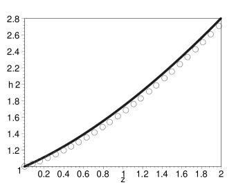
Figure 1: The dimensionless Hubble parameter $h$ with redshift $z$. The circled line is for the standard $\Lambda\textrm{CDM}$ model. The solid line is for the aether model.

Figure 2: The deceleration parameter $q$ with redshift $z$. The circled line is for the standard $\Lambda\textrm{CDM}$ model. The solid line is for the aether model.

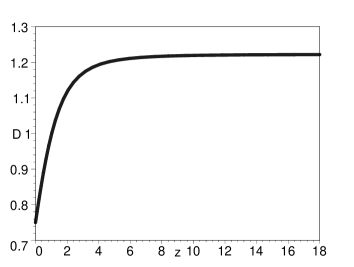
Figure 3: The dimensionless energy density $D$ with redshift $z$. At redshifts greater than $4$, the energy density of aether field is nearly a constant.

In Fig. 3, we plot the dimensionless energy density (from Eq. (25))

$$D=\zeta^{2}\left(3-\frac{1}{h}\frac{d{h}}{dx}\right)^{2}\;,$$ (27)

for the aether field with the redshift. It shows the energy density of aether field is nearly a constant at redshifts greater than $4$.

Carroll et al carroll:2004 showed that the energy density of aether field is proportional to $H^{2}$ in the absence of gravitational coupling. The reason for this difference could be understood as follows: for the usual Einstein-aether theory, the norm constraint condition Eq. (4) gives (by order) in flat FRW Universe carroll:2004

$$A^{\mu}\sim m\;.$$ (28)

The norm of the vector is fixed as a constant. On the other hand, dimensional analysis suggests that we must have

$$\nabla_{\mu}\sim H\;.$$ (29)

Therefore, we conclude that the energy density is

$$\nabla_{\mu}A^{\mu}\nabla_{\nu}A^{\nu}\sim H^{2}\;,$$ (30)

which is consistent with the calculation of Ref. carroll:2004 . For our Einstein-aether field, from the constraint equation Eq. (7)

$$A^{\mu}\sim\frac{m}{H}\sim\frac{m}{\sqrt{\rho}}\;,$$ (31)

where $\rho$ is the total energy of the Universe. It is apparent that the norm of our vector is environment dependant. The energy density turns out to be

$$\nabla_{\mu}A^{\mu}\nabla_{\nu}A^{\nu}\sim H^{2}\cdot H^{-2}\simeq{\rm const.}\;$$ (32)

As another example, we have checked with detailed calculation that for the Einstein-aether theory with the Lagrangian density

$$\mathscr{L}=\sqrt{-g}\left[G_{\mu\nu}\nabla^{\mu}A^{\alpha}\nabla^{\nu}A_{\alpha}+\lambda\left(G_{\mu\alpha}G^{\alpha}_{\nu}A^{\mu}A^{\nu}+m^{2}\right)\right]\;,$$ (33)

the energy density of aether in this model is also kept at nearly constant level. However, the corresponding Einstein equations involves derivatives higher than second order.

III Cosmological constant and Phantom from quintessence

III.1 equation of motion

Inspired by the dynamical behavior of the Einstein-aether theory with the Lagrange multiplier field, we consider its role in quintessence field theory. For our purpose, here we consider the following model:

$$\mathscr{L}=-\sqrt{-g}\left[\frac{1}{2}G_{\mu\nu}\nabla^{\mu}\phi\nabla^{\nu}\phi+\lambda\left(\frac{1}{2}R\phi+\frac{m^{2}}{2}\right)\right]\;$$ (34)

where $m$ is a constant, $R$ is the Ricci scalar. The case where $\lambda$ is a constant has been investigated extensively. However, we emphasize that $\lambda$ is not a constant, but a Lagrange multiplier or auxiliary field. This brings interesting new possibilities.

The equation of motion for $\lambda$ and $\phi$ are given by

$$R\phi+m^{2}=0\;,$$ (35)

$$G_{\mu\nu}\nabla^{\mu}\nabla^{\nu}\phi-\frac{\lambda}{2}R=0\;,$$ (36)

and the energy-momentum tensor takes the form sushkov:2009 ; ford:1987 ; uzan:1999

$$T_{\mu\nu} = -{\textstyle\frac{1}{2}}\nabla_{\mu}\phi\,\nabla_{\nu}\phi\,R+2\nabla_{\alpha}\phi\,\nabla_{(\mu}\phi R^{\alpha}_{\nu)}$$ (37)

$$+\nabla^{\alpha}\phi\,\nabla^{\beta}\phi\,R_{\mu\alpha\nu\beta}+\nabla_{\mu}\nabla^{\alpha}\phi\,\nabla_{\nu}\nabla_{\alpha}\phi$$

$$-\nabla_{\mu}\nabla_{\nu}\phi\,\square\phi-{\textstyle\frac{1}{2}}(\nabla\phi)^{2}G_{\mu\nu}$$

$$+g_{\mu\nu}\big{[}-{\textstyle\frac{1}{2}}\nabla^{\alpha}\nabla^{\beta}\phi\,\nabla_{\alpha}\nabla_{\beta}\phi+{\textstyle\frac{1}{2}}(\square\phi)^{2}$$

$$-\nabla_{\alpha}\phi\,\nabla_{\beta}\phi\,R^{\alpha\beta}\big{]}-{\textstyle\frac{1}{2}}\lambda m^{2}g_{\mu\nu}+\lambda G_{\mu\nu}\phi$$

$$+\lambda g_{\mu\nu}\nabla^{2}\phi-\lambda\nabla_{(\mu}\nabla_{\nu)}\phi\;.$$

III.2 cosmological solution

With the flat FRW background model, we obtain

$$\phi = -\frac{m^{2}}{{R}}=\frac{m^{2}}{{{6\dot{H}+12H^{2}}}}\;,$$ (38)

$$\lambda = \frac{2}{m^{2}}\phi\left[3H^{2}\ddot{\phi}+3H\left(2\dot{H}+3H^{2}\right)\dot{\phi}\right]\;.$$ (39)

From the energy-momentum tensor, the energy density of scalar is

$$\rho_{\phi}=\frac{9}{2}H^{2}\dot{\phi}^{2}+3\lambda H^{2}\phi+3\lambda H\dot{\phi}+\frac{1}{2}\lambda m^{2}$$ (40)

Using Eq. (38) and Eq. (39), and assuming the total equation of state $w$ is a constant, we find the energy density is

$$\rho_{\phi}=18{m^{4}}\cdot\frac{\left(1+w\right)\left(1-w-w^{2}\right)}{\left(1-3w\right)^{3}}\;.$$ (41)

We have $w\simeq 0$ for the matter dominated Universe. The corresponding energy density is

$$\rho_{\phi}=18m^{4}\;.$$ (42)

This density does not vary as the Universe expands, so the field behaves as a cosmological constant.

For the radiation dominated case, we have $n\simeq 1/2$. It is apparent that Eq. (41) is divergent. This is not surprising, since $R=0$ in radiation dominated Universe. We should look for the energy density from the Lagrangian. Ref. gao:2010 showed that the energy density scales as

$$\rho_{\phi}=\frac{\rho_{0}}{a^{2}}\;,$$ (43)

in the radiation dominated epoch, with $\rho_{0}$ an integration constant. Then the field has the equation of state $w=-1/3$. The energy density evolution given in Eq. (41) is different from the usual non-minimally coupled quintessence field. For the present-day Universe, we have $w\simeq{-0.75}$ such that $\rho_{\phi}\simeq 0.16\ m^{2}.$

The reason for this difference could be understood as follows. The fixed-norm constraint Eq. (35) (also Eq. (38)) tells us

$$\phi\sim\frac{m^{2}}{H^{2}}\sim\frac{m^{2}}{{\rho}}\;.$$ (44)

In other words, the strength of the field is determined by the energy density of the background matter source. In the usual quintessence theory, the strength of the field can be arbitrarily large. However, we have $\nabla_{\mu}\sim H$ and $G_{\mu\nu}\sim H^{2}$, so

$$G_{\mu\nu}\nabla^{\mu}\phi\nabla^{\mu}\phi\sim H^{2}\cdot H^{2}\cdot H^{-4}\sim{\rm const.}\;$$ (45)

Another interesting model is

$$\mathscr{L} = -\sqrt{-g}\left[\frac{1}{2}\nabla_{\mu}\phi\nabla^{\mu}\phi+\lambda\left(\frac{1}{2}R\phi+\frac{m^{2}}{2}\right)\right]\;,$$ (46)

in this case the scalar field behaves as “phantom”, with equation of state $w<-1$. This can be seen by the following reasoning: the norm-fixing constraint yields

$$\phi\sim\frac{m}{H^{2}}\;.$$ (47)

So the energy density is

$$\nabla_{\mu}\phi\nabla^{\mu}\phi\sim H^{2}\cdot{H^{-4}}\sim H^{-2}\;.$$ (48)

The energy density increases with the expansion of the Universe, i.e. it behaves as a phantom. By using the Lagrange Multiplier field, one may construct the dark energy model which exhibit the desired behaviors.

IV cold dark matter from quintessence

IV.1 the theory

In Section II and Section III, we have shown that the energy density of the Einstein-aether and the quintessence can be kept at nearly a constant value in the evolution of the Universe by employing a Lagrange multiplier field, which points to a dynamical origin of cosmological constant. In this section, we shall show that with proper choice of the Lagrange multiplier field, the cold dark matter behavior can also be obtained.

Note that the usual quintessence field can have zero pressure for particular potential forms. However, the sound speed for the canonical quintessence field is 1, so it is not a true cold dark matter. Here we show how with the help of Lagrange multiplier field, we can construct true cold dark matter with the quintessence field.

We consider the following Lagrangian density:

$$\mathscr{L} = -\lambda\sqrt{-g}\left[\frac{1}{2}\nabla_{\mu}\phi\nabla^{\mu}\phi+V\left(\phi\right)\right]\;,$$ (49)

where $\lambda$ is a Lagrange multiplier field, and $V\left(\phi\right)$ is the scalar potential. The equation of motion for $\lambda$ and $\phi$ are given by

$$\frac{1}{2}\nabla_{\mu}\phi\nabla^{\mu}\phi+V\left(\phi\right)=0\;,$$ (50)

$$\nabla_{\mu}\left(\lambda\nabla^{\mu}\phi\right)-\lambda V^{{}^{\prime}}=0\;,$$ (51)

Here prime denotes the derivative with respect to $\phi$. The energy-momentum tensor is

$$T_{\mu\nu}=\lambda\left[\nabla_{\mu}\phi\nabla_{\nu}\phi-\frac{1}{2}g_{\mu\nu}\nabla_{\alpha}\phi\nabla^{\alpha}\phi-g_{\mu\nu}V\right]\;.$$ (52)

For a flat FRW model, Eq. (50) and Eq. (51) reduce to

$$\frac{1}{2}\dot{\phi}^{2}-V=0\;,$$ (53)

and

$$\ddot{\phi}+3H\dot{\phi}+V^{{}^{\prime}}+{\lambda}^{-1}\dot{\lambda}\dot{\phi}=0\;.$$ (54)

Differentiating Eq. (53) with respect to time $t$, we obtain

$$V^{{}^{\prime}}=\ddot{\phi}\;.$$ (55)

Substituting it into Eq. (54), we obtain

$$\frac{d\dot{\phi}}{\dot{\phi}}+\frac{3}{2}\frac{da}{a}+\frac{1}{2}\frac{d\lambda}{\lambda}=0\;.$$ (56)

Solving the equation, we have

$$\lambda=\frac{\rho_{0}}{a^{3}\dot{\phi}^{2}}\;,$$ (57)

with $\rho_{0}$ an integration constant. Using Eq. (52) and Eq. (57), we find that the energy density evolves as

$$\rho_{\phi}=\frac{\rho_{0}}{a^{3}}\;,$$ (58)

which is exactly the behavior of the cold dark matter. We note that this expression of energy density is independent of the explicit form of the scalar potential.

IV.2 speed of sound

A dark matter model will fit the CMB data only if the rest-frame sound speed is indeed zero mydeg . As this is such an important condition, it is worthwhile to spend some time to derive the sound speed from the perturbation equations directly. For this purpose, we work in the Newtonian gauge. In the absence of anisotropic stress, and for scalar perturbations, the perturbed flat FRW metric can be written in the form

$$ds^{2}=-\left(1+2\Phi\right)dt^{2}+a\left(t\right)^{2}\left(1-2\Phi\right)dx_{i}dx^{i}\;,$$ (59)

where $\Phi$ is the Newtonian potential. For the scalar field and the Lagrange multiplier field, we define the perturbation as

$$\phi\left(t,\vec{x}\right) = \phi_{0}\left(t\right)+\delta\phi\left(t,\vec{x}\right)\;,$$ (60)

$$\lambda\left(t,\vec{x}\right) = \lambda_{0}\left(t\right)+\delta\lambda\left(t,\vec{x}\right)\;.$$ (61)

The perturbed energy-momentum tensor is

$$\delta T_{0}^{0} = \delta\rho_{\phi}=\lambda\left(\dot{\phi_{0}}\dot{\delta\phi}-\Phi\dot{\phi_{0}}^{2}+V^{{}^{\prime}}\delta\phi\right)+\rho_{\phi 0}\delta\lambda/\lambda\;,$$

$$\delta T_{i}^{j} = -\delta p_{\phi}\left(t,\vec{x}\right)\delta_{i}^{j}=-\lambda\left(\dot{\phi_{0}}\delta\dot{\phi}-\Phi\dot{\phi_{0}}^{2}-V^{{}^{\prime}}\delta\phi\right)\delta_{i}^{j}\;,$$

$$ik\delta T_{0}^{i} = ik\left(\rho_{\phi 0}+p_{\phi 0}\right)\delta u^{i}_{\phi}\left(t,\vec{x}\right)={\rho_{\phi 0}}\mathscr{V}\;.$$ (62)

It is well-known that both the adiabatic sound speed and the rest frame sound speed (the sound speed for the fluid in its rest frame) play important roles in the discussion of structure formation theory. Here we work out both of these quantities explicitly. The adiabatic sound speed squared is defined as bean:2004 ; kunz:2006

$$c_{a}^{2}\equiv\frac{\dot{p}_{\phi 0}}{\dot{\rho}_{\phi 0}}.$$ (63)

Since the pressure of this quintessence is vanishing, we conclude that

$$c_{a}^{2}=0.$$ (64)

The rest frame sound speed squared $\hat{c}_{s}^{2}$ of the scalar is related to the pressure perturbation in the Newtonian gauge through bean:2004 ; kunz:2006

$$\delta p_{\phi}=\hat{c}_{s}^{2}\delta\rho_{\phi}+\frac{3aH}{k^{2}}\left(\hat{c}_{s}^{2}-c_{a}^{2}\right){\rho_{\phi 0}}\mathscr{V}\;.$$ (65)

Taking into account of $c_{a}^{2}=0$, we can rewrite Eq. (65) as

$$\delta p_{\phi}=\hat{c}_{s}^{2}\left(\delta\rho_{\phi}+\frac{3aH}{k^{2}}{\rho_{\phi 0}}\mathscr{V}\right)\;.$$ (66)

In order to calculate $\delta p_{\phi}$, we resort to the equation of motion for the scalar field perturbations. To this end, we insert the expansions Eq. (60-61) into the Lagrangian density, and expand to quadratic order

$$\mathscr{L}\rightarrow\mathscr{L}_{0}+\mathscr{L}_{1}+\mathscr{L}_{2}\;,$$ (67)

where $\mathscr{L}_{1}$ and $\mathscr{L}_{2}$ are the Lagrangian terms which are of linear and quadratic order in $\delta\phi$, respectively. Variation of $\mathscr{L}_{0}$ give us the equation of motions for the unperturbed $\phi$ and $\lambda$. Variation of $\mathscr{L}_{2}$ give us the equation of motion for $\delta\phi$ and $\delta\lambda$, respectively. Variation of $\mathscr{L}_{1}$ does not yield new information.

Straightforward calculation yields

$$\mathscr{L}_{2} = -a^{3}\delta\lambda\left(\Phi\dot{\phi}_{0}^{2}-\dot{\phi}_{0}\delta\dot{\phi}+V^{{}^{\prime}}\delta\phi\right)$$ (68)

$$-2a^{3}\Phi\delta\lambda\left(-\frac{1}{2}\dot{\phi}^{2}+V\right)$$

$$+2a^{3}\Phi\lambda\left(\Phi\dot{\phi}_{0}^{2}-\dot{\phi}_{0}\delta\dot{\phi}+V^{{}^{\prime}}\delta\phi\right)$$

$$-\lambda a^{3}\left[2\Phi\dot{\phi}_{0}\delta\dot{\phi}-\frac{1}{2}\delta\dot{\phi}^{2}+\frac{1}{2a^{2}}\left(\nabla\delta{\phi}\right)^{2}\right.$$

$$\left.+\frac{1}{2}V^{{}^{\prime\prime}}\delta{\phi}^{2}\right]\;.$$

Variation of $\mathscr{L}_{2}$ with respect to $\delta\lambda$ and taking into account of Eq. (53), we obtain

$$\Phi\dot{\phi}_{0}^{2}-\dot{\phi}_{0}\delta\dot{\phi}+V^{{}^{\prime}}\delta\phi=0\;.$$ (69)

Comparing this with the second equation in Eqs. (IV.2), it follows that

$$\delta T_{i}^{j} = -\delta p_{\phi}\left(t,\vec{x}\right)\delta_{i}^{j}=0\;.$$ (70)

We then conclude immediately that

$$\hat{c}_{s}^{2}=0\;.$$ (71)

Therefore, for this model the pressure, the adiabatic sound speed, and the rest frame sound speed all vanishes, which ensures that the scalar field has every desirable property of the cold dark matter.

V conclusion and discussion

In conclusion, we have introduced gravitational coupling to the usual Einstein-aether theory and Lagrange multiplier field to the scalar field quintessence theory. We find that by changing the norm-fixing condition from unit norm in the usual Einstein aether theory to an environment-dependent one, one can make the aether density stay constant as the Universe expands.

As for the case of scalar field quintessence, by introducing the Lagrange multiplier field, the strength of the quintessence field can be related to the background matter source, and the density can also be kept as nearly constant during the cosmic expansion. This suggests a possible dynamical origin of cosmological constant. Alternatively, we also find an example in which the quintessence with Lagrange multiplier field behaves as phantom.

Furthermore, with the help of a Lagrange multiplier field, we also proposed a way to generate cold dark matter from quintessence. It is found that the pressure, the adiabatic sound speed and the rest-frame sound speed of the quintessence is exactly zero. These properties enable the scalar field to be a potential candidate for cold dark matter.

- (1) S. Perlmutter et al., Astrophys. J. 517, 565 (1999)
- (2) A. G. Riess et al., Astron. J. 116, 1009 (1998)
- (3) R. R. Caldwell, R. Dave and P. J. Steinhardt, Phys. Rev. Lett. 80, 1582 (1998) [astro-ph/9708069]; C. Wetterich, Nucl. Phys. B 302, 668 (1988); P. J. E. Peebles and B. Ratra, Astrophys. J. 325, L17 (1988).
- (4) R. R. Caldwell, Phys Lett. B 545 (2002) 23.
- (5) S. M. Carroll, M. Hoffman and M. Trodden, Phys. Rev. D 68, 023509 (2003); B. Feng, X. L. Wang and X. M. Zhang, Phys. Lett. B 607, 35 (2005) [astro-ph/0404224]; E. Elizalde, S. Nojiri and S. D. Odintsov, Phys. Rev. D 70, 043539 (2004); B. Feng, M. Li, Y. S. Piao and X. M. Zhang, Phys. Lett. B 634, 101 (2006) [astro-ph/0407432];
- (6) T. Chiba, T. Okabe and M. Yamaguchi, Phys. Rev. D 62, 023511 (2000); C. Armendariz-Picon, V. F. Mukhanov and P. J. Steinhardt, Phys. Rev. Lett. 85, 4438 (2000) [astro-ph/0004134]; C. Armendariz-Picon, V. F. Mukhanov and P. J. Steinhardt, Phys. Rev. D 63, 103510 (2001) [astro-ph/0006373].
- (7) M. Li, Phys.Lett. B603 (2004) 1.
- (8) S. Nojiri and S. D. Odintsov, Gen. Rel. Grav. 38, 1285 (2006); X. Zhang, F. Q. Wu, Phys. Rev. D 72 (2005) 043524; Z. Chang, F.Q. Wu, X. Zhang, Phys.Lett.B 633 (2006) 14; J. Zhang, X. Zhang, H. Liu Phys.Lett.B651 (2007) 84; Y. Ma, X. Zhang, Phys.Lett.B 661 (2008) 239; L. Xu, W. Li J. Lu arXiv: 0810.4730; C. Gao, F. Wu, X. Chen and Y. Shen, Phys. Rev. D 79, 043511 (2009). R. G. Cai, B. Hu and Y. Zhang, Commun. Theor. Phys. 51, 954 (2009) C.J. Feng, Phys. Lett. B 670, 231 (2008); L.N. Granda and A. Oliveros, Phys. Lett. B 669, 275 (2008); Q.G. Huang and M. Li, JCAP 0408, 013 (2004); Y.G. Gong, B. Wang and Y.Z. Zhang Phys. Rev. D 72, 043510 (2005); B. Wang, Y.G. Gong and E. Abdalla, Phys. Lett. B 624, 141 (2005); B. Chen, M. Li and Y. Wang, Nucl. Phys. B 774, 256 (2007); I.P. Neupane, Phys. Rev. D 76, 123006 (2007); J.P. Wu, D.Z. Ma and Y. Ling, Phys. Lett. B 663, 152 (2008); H. Wei and R.G. Cai, Eur. Phys. J. C 59, 99 (2009).
- (9) R. G. Cai, Phys. Lett. B 657, 228 (2007).
- (10) H. Wei and R. G. Cai, Phys. Lett. B 660, 113 (2008).
- (11) T. Jacobson and D. Mattingly, Phys. Rev. D 64, 024028 (2001) [arXiv:grqc/ 0007031];
- (12) V. A. Kostelecky and S. Samuel, Phys. Rev. D40, 1886 (1989); V. A. Kostelecky, Phys. Rev. D69, 105009 (2004), hep-th/0312310; J. D. Bekenstein, (2004), astro-ph/0403694; J.W. Elliott, G. D. Moore and H. Stoica, JHEP 0508, 066 (2005) [arXiv:hepph/ 0505211]; See, for example, M. Gasperini, Class. Quantum Grav. 4, 485 (1987); Repulsive gravity in the very early Universe, Gen. Rel. Grav. 30, 1703 (1998); and references therein; B. Li and H. zhao, Phys. Rev. D 80, 064007 (2009).
- (13) S. Nojiri and S. D. Odintsov, Phys. Rev. D 68, 123512 (2003); S. Nojiri and S. D. Odintsov, Int. J. Geom. Meth. Mod. Phys. 4, 115 (2007); M. Israelit and N. Rosen, Found. Phys. 22, 555 (1992); M. Israelit and N. Rosen, Found. Phys. 24, 901 (1994); G. R. Dvali, G. Gabadadze and M. Porrati, Phys. Lett. B 485, 208 (2000); C. Deffayet, G. R. Dvali and G. Gabadadze, Phys. Rev. D 65, 044023 (2002); S. M. Carroll, V. Duvvuri, M. Trodden and M. S. Turner, Phys. Rev. D 70, 043528 (2004); J. D. Bekenstein, Phys. Rev. D 70, 083509 (2004); [Erratum-ibid. D 71, 069901 (2005)]; C. Skordis, D. F. Mota, P. G. Ferreira and C. Boehm, Phys. Rev. Lett. 96, 011301 (2006).
- (14) R. R. Caldwell, M. Kamionkowski, Ann. Rev. Nucl. Part. Sci. 59, 397 (2009).
- (15) C.M. Will and K. Nordvedt, Jr., Astrophys. J. 177, 757 (1972); K. Nordvedt, Jr. and C.M. Will, Astrophys. J. 177, 775 (1972); R.W. Hellings and K. Nordvedt, Jr., Phys. Rev. D7, 3593 (1973).
- (16) Sean. M. Caroll, et al, Phys. Rev. D 79, 065011 (2009).
- (17) Sean. M. Caroll, et al, Phys. Rev. D 79, 065012 (2009).
- (18) Sean. M. Carroll and Eugene. A. Lim, Phys. Rev. D 70, 123525 (2004).
- (19) V. F. Mukhanov and R. H. Brandenberger, Phys. Rev. Lett. 68, 1969 (1992); R. H. Brandenberger, V. F. Mukhanov and A. Sornborger, Phys. Rev. D 48, 1629 (1993). arXiv:gr-qc/9303001.
- (20) Eugene A. Lim, Ignacy Sawicki, Alexander Vikman, JCAP 05, 012 (2010); arXiv:astro-ph/1003.5751.
- (21) S. Capozziello, J. Matsumoto, S. Nojiri and S. D. Odintsov, Phys. Lett. B 693, 2010 (198).
- (22) S. Nojiri and S. D. Odintsov, Phys. Lett. B 691, 2010 (60); S. Nojiri and S. D. Odintsov, Phys. Rev. D 83, 2011 (023001).
- (23) Y. F. Cai and E. N. Saridakis, Class. Quant. Grav. 28, 035010 (2011).
- (24) C. J. Feng and X. Z. Li, JCAP 1010, 027 (2010).
- (25) J. Kluson, Class. Quant. Grav. 28, 125025 (2011).
- (26) S. Nojiri et al., Phys. Lett. B 696, 2011 (278).
- (27) S. Nojiri and S. D. Odindtsov, “Unified cosmic history in modified gravity: from F(R) theory to Lorentz non-invariant models”, arXiv:1011.0544.
- (28) K.Bambo et al., “Screening of cosmological constant for De Sitter Universe in non-local gravity, phantom-divide crossing and finite-time future singularities”, arXiv:1104.2692.
- (29) J. Kluson et al., “Covariant Lagrange multiplier constrained higher derivative gravity with scalar projectors”, arXiv:1104.4286.
- (30) C. Armendariz-Picon and A. Diez-Tejedor, JCAP 0912, 018 (2009) astro-ph/0904.0809.
- (31) E. Komatsu et al, Astrophys. J. Suppl. 180, 330 (2009).
- (32) S. V. Sushkov, Phys. Rev. D 80, 103505 (2009).
- (33) L. H. ford, Phys. Rev. D 35, 2339 (1987).
- (34) J. P. Uzan, Phys. Rev. D 59, 123510 (1999).
- (35) C. Gao, JCAP 6, 23 (2010); arXiv:gr-qc/1002.4035.
- (36) M. Kunz, arXiv:astro-ph/0702615.
- (37) R. Bean and O. Dor e, Phys. Rev. D69, 083503 (2004)
- (38) M. Kunz and D. Sapone, Phys. Rev. D74, 123503 (2006).