Localization of a Bose-Einstein condensate vortex in a bichromatic optical lattice

Abstract

By numerical simulation of the time-dependent Gross-Pitaevskii equation we show that a weakly interacting or noninteracting Bose-Einstein condensate (BEC) vortex can be localized in a three-dimensional bichromatic quasi-periodic optical-lattice (OL) potential generated by the superposition of two standing-wave polarized laser beams with incommensurate wavelengths. This is a generalization of the localization of a BEC in a one-dimensional bichromatic OL as studied in a recent experiment [Roati et al., Nature 453, 895 (2008)]. We demonstrate the stability of the localized state by considering its time evolution in the form of a stable breathing oscillation in a slightly altered potential for a large period of time. Finally, we consider the localization of a BEC in a random 1D potential in the form of several identical repulsive spikes arbitrarily distributed in space.

I Introduction

The possibility of the localization of the electronic wave function in a one-dimensional (1D) disordered potential as predicted by Anderson in his pioneering work anderson has drawn the attraction of researchers in different areas. Different forms of localization have been observed experimentally in diverse contexts, such as in electromagnetic waves light ; micro , in sound waves sound , and also more recently in quantum matter waves billy ; roati ; chabe ; edwards . Using a cigar-shaped noninteracting Bose-Einstein condensate (BEC) book1 ; book2 of ⁸⁷Rb atoms, Billy et al. billy demonstrated its exponential localization when released into a 1D waveguide in the presence of a controlled disorder created by a laser speckle. In another experiment, using a cigar-shaped noninteracting BEC of ³⁹K atoms, Roati et al. roati demonstrated its localization in a 1D bichromatic optical-lattice (OL) potential created by the superposition of two standing-wave polarized laser beams with different wavelengths. The noninteracting BEC of ³⁹K atoms was created roati by tuning the inter-atomic scattering length to zero near a Feshbach resonance fesh .

The localization of a BEC in a 1D bichromatic quasi-periodic OL potential and related topics have been the subject matter of several theoretical das ; dnlse ; harper ; boers ; aubry ; thouless ; random ; optical ; modugno ; modugno2 ; roux ; roscilde ; paul ; adhikari and experimental billy ; roati ; chabe ; edwards studies. After the pioneering experiments roati ; billy on the localization of a 1D cigar-shaped BEC, a natural extension of this phenomenon would be to achieve localization in higher dimensions, e.g., in two (2D) and three (3D) dimensions. We address this important issue in the present investigation. Using the complete numerical solution of the Gross-Pitaevskii (GP) equation GP , here we study the localization of a (nonrotating) disk-shaped BEC in 2D and also a BEC in 3D, with a small nonlinearity, in the presence of bichromatic OL potentials along orthogonal directions. (For zero nonlinearity the problem of a stationary state of a $d$-dimensional $-$ $d=2,3$ $-$ nonrotating BEC trivially decouples into $d$ 1D problems and for a large repulsive nonlinearity the localization is destroyed adhikari ; modugno2 .) In 3D another nontrivial phenomenon can happen, i.e., the generation of a stable vortex state of unit quantum. Here we demonstrate the localization of a stable nontrivial vortex state in a 3D BEC under the action of bichromatic OL potential along the axial direction and harmonic potentials along radial directions. We find, as in 1D adhikari ; modugno2 , a repulsive nonlinearity has a strong effect on localization and a not-too-large nonlinearity destroys localization in all cases. We exhibit results for zero and small nonlinearities. (Effects of a weak nonlinearity in Anderson localization have been shown experimentally in light waves in photonic crystals roati ; lahini .)

In the presence of strong disorder, the localized state could be quite similar to a localized state of Gaussian shape in an infinite potential. However, the more interesting case of localization is in the presence of a weak disorder when the system is localized due to the quasi-periodic nature of the potential billy ; roati and not due to the strength of the lattice. When this happens the localized state acquires an exponential tail. The present localization with an exponential tail in a quasi-periodic OL potential with a deterministic weak disorder is a special case of Anderson localization in a fully disordered potential and is well described in the Aubry-André model aubry .

In the pioneering study, Anderson considered localization of electron(s) in a 1D random potential generated by impurity or disorder arbitrarily distributed on a lattice. This is of interest in the study of a BEC and we consider its localization in a disorder potential in the form of identical narrow repulsive spikes (simulating delta functions) distributed randomly in space. (This is different from a speckle potential where the spikes also have different strength and width.) We find that as small as four such spikes can localize a noninteracting BEC in 1D. This is not just of academic interest as such potential can be created in 1D and possibly in 2D for a BEC in an atom chip chip ; chip2 . A single repulsive spike separating the BEC into two parts is now routinely created chip2 .

There have been theoretical studies on different aspects of Anderson localization which are worth mentioning adhikari . Wobst et al. wobst considered Anderson localization in higher dimensions. Sanchez-Palencia et al. and Clément et al. considered Anderson localization in a random potential random ; stoca ; optical . Damski et al. and Schulte et al. considered Anderson localization in disordered OL potential optical . There have been studies of Anderson localization with other types of disorder other . Effect of interaction on Anderson localization was also studied interaction ; dnlse . Anderson localization in BEC under the action of a disordered potential in 2D and 3D has also been investigated 2D3D .

In Sec. II we present a brief account of the nonlinear 2D and 3D time-dependent GP equations used in our study and of the variational solution of the same under appropriate conditions. The generalization of the equation to study vortex states in 3D is also presented. In Sec. III we present numerical results of localization employing time propagation using the semi-implicit Crank-Nicolson algorithm. The wave function of the localized states has a central Gaussian (variational) form with a long exponential tail. First we consider in Sec. III.1 the localization of a 2D disk-shaped BEC. We also consider localization of a 3D BEC and a 3D vortex BEC in bichromatic OL potential(s) in Sec. III.2. In Sec. III.3 we consider the localization of a noninteracting BEC for a random potential comprised of arbitrarily distributed narrow spikes. In Sec. IV we present a brief discussion and concluding remarks.

II Theoretical formulation of localization

The quasi-periodic bichromatic OL potentials generated by two standing-wave polarized laser beams of incommensurate wavelengths in the $x$ direction have the following generic forms roati :

$$U(x)=\sum_{i=1}^{2}s_{i}E_{i}\cos^{2}(k_{i}x),$$ (1)

$$U(x)=\sum_{i=1}^{2}s_{i}E_{i}\sin^{2}(k_{i}x),$$ (2)

where $s_{i},i=1,2,$ are the amplitudes of the OL potentials in units of respective recoil energies $E_{i}=2\pi^{2}\hbar^{2}/(m\lambda_{i}^{2})$, and $k_{i}=2\pi/\lambda_{i}$, $i=1,2$ are the respective wave numbers and $\lambda_{i}$ are the wave lengths, $\hbar(\equiv h/2\pi)$ is the reduced Planck constant, and $m$ the mass of an atom.

If we have a single periodic potential of forms (1) and (2) with $s_{2}=0,$ the solution of the Schrödinger equation cannot be localized. One can have localization if a second periodic component with a different frequency is introduced in Eqs. (1) and (2). These localized states are not the gap solitons, which are localized states in the solution of a nonlinear Schrödinger equation with a repulsive nonlinearity appearing in the band-gap of the spectrum of the linear Schrödinger equation gs .

The BEC in 3D is described by the GP equation

$$i\hbar\frac{\partial\phi({\bf r},\tau)}{\partial\tau}=\left[-\frac{\hbar^{2}\nabla^{2}}{2m}+V({\bf r})+g|\phi({\bf r},\tau)|^{2}\right]\phi({\bf r},\tau),$$ (3)

where $g=4\pi\hbar^{2}aN/m,\int|\phi({\bf r},\tau)|^{2}d{\bf r}=1$, $\tau$ the time, $N$ the number of atoms, $V({\bf r})$ is the trap, and $a$ is the atomic scattering length. With three quasi-periodic, bichromatic OL potential in $x,y$, and $z$ directions, after canceling the factor $\hbar^{2}/m$ from both sides of Eq. (3), the GP equation in explicit notation becomes

$$i\frac{\partial\phi(x,y,z,t)}{\partial t} = \biggr{[}-\frac{1}{2}\left(\partial_{x}^{2}+\partial_{y}^{2}+\partial_{z}^{2}\right)+V(x)+V(y)$$ (4)

$$+ V(z)+g|\phi(x,y,z,t)|^{2}\biggr{]}\phi(x,y,z,t),$$

where $g=4\pi aN$, $\partial_{x}$’s denote space derivatives, and time $t\equiv\tau\hbar/m$ is now expressed in units of $m/\hbar$. Note that Eq. (4) is not expressed in dimensionless units. The variables $x,y,z,\lambda_{i}$ are in actual units of length ($L$), $|\phi|^{2}$ is in units of $L^{-3}$ with normalization $\int_{-\infty}^{\infty}\int_{-\infty}^{\infty}\int_{-\infty}^{\infty}|\phi(x,y,z,t)|^{2}dxdydz=1$. In Eq. (4) the scaled potentials $V(x)\equiv U(x)m/\hbar^{2}$ are now defined by one of the two following expressions:

$$V(x) = \sum_{i=1}^{2}\frac{2\pi^{2}s_{i}}{\lambda_{i}^{2}}\cos^{2}\left(\frac{2\pi x}{\lambda_{i}}\right),$$ (5)

$$V(x) = \sum_{i=1}^{2}\frac{2\pi^{2}s_{i}}{\lambda_{i}^{2}}\sin^{2}\left(\frac{2\pi x}{\lambda_{i}}\right).$$ (6)

In case of a 2D and 3D BEC, instead of having the same potential, e.g., (5) or (6) in different directions, one can choose different potentials along different directions.

For axially-symmetric traps, the GP equation can be easily generalized to include a vortex state, as shown in Ref. ds ; book2 , in axially-symmetric coordinates ${\bf r}\equiv(\rho,z),$ where $\rho$ is the radial coordinate and $z$ the axial coordinate. To obtain a singly quantized vortex state of angular momentum $\hbar$ around $z$ axis, one has to explicitly introduce a phase (equal to the azimuthal angle) in the wave function. (Vortex states of higher angular momentum are unstable and decays into multiple states of angular momentum $\hbar$.) This procedure introduces a centrifugal term in the GP equation representing a vortex state ds ; book2 . Thus we can study a localized quantized BEC vortex of unit angular momentum in the axially-symmetric potential, where the bichromatic OL potential $V(z)$ is placed along the axial $z$ direction and an harmonic trap $\rho^{2}/2$ along the transverse radial $\rho$ direction. The modified GP equation for such a vortex is given by ds

$$i\frac{\partial\phi(\rho,z,t)}{\partial t}=\biggr{[}-\frac{1}{2}\frac{\partial^{2}}{\partial\rho^{2}}-\frac{1}{2\rho}\frac{\partial}{\partial\rho}-\frac{1}{2}\frac{\partial^{2}}{\partial z^{2}}+\frac{1}{2\rho^{2}}$$

$$+\frac{1}{2}\rho^{2}+V(z)+g|\phi(\rho,z,t)|^{2}\biggr{]}\phi(\rho,z,t),$$ (7)

where we have explicitly included the angular momentum dependent centrifugal term ${1}/({2\rho^{2}})$ ajp . Because of the centrifugal term, the density of the vortex should be zero along the $z$ axis.

If there is a strong harmonic trap in the axial $z$ direction, one can derive a reduced quasi-2D GP equation for a disk-shaped BEC, which can be written in dimensionless harmonic oscillator units as CPC

$$i\frac{\partial\phi(x,y,t)}{\partial t} = \biggr{[}-\frac{1}{2}\left(\partial_{x}^{2}+\partial_{y}^{2}\right)+V(x)+V(y)$$ (8)

$$+ g|\phi(x,y,t)|^{2}\biggr{]}\phi(x,y,t),$$

where $g=2\sqrt{2\pi}aN$ and $V(x)$ is given by Eqs. (5) or (6). In Eq. (8) the normalization is $\int_{-\infty}^{\infty}\int_{-\infty}^{\infty}|\phi(x,y,t)|^{2}dxdy=1$. In Eq. (8) lengths are expressed in units of $l_{z}\equiv\sqrt{\hbar/m\omega_{z}}$ with $\omega_{z}$ the frequency in $z$ direction, $\phi(x,y,t)$ in units of $l_{z}^{-2}$ and time in units of $\omega_{z}^{-1}$.

Finally, for the sake of completeness we note that if there is a strong harmonic trap in transverse $y$ and $z$ directions, one can derive a reduced quasi-1D GP equation for a cigar-shaped BEC, which can be written in dimensionless harmonic oscillator units as CPC

$$i\frac{\partial\phi(x,t)}{\partial t}=\biggr{[}-\frac{1}{2}\partial_{x}^{2}+V(x)+g|\phi(x,t)|^{2}\biggr{]}\phi(x,t),$$ (9)

where $g=2aN$ and $V(x)$ is given by Eqs. (5) or (6). Now the normalization is $\int_{-\infty}^{\infty}|\phi(x,t)|^{2}dx=1$. Equation (9) has been used modugno ; adhikari for the study of localization in 1D in bichromatic OL potential. In Eq. (9) lengths are expressed in units of $l\equiv\sqrt{\hbar/m\omega_{\perp}}$ with $\omega_{\perp}$ the frequency in transverse $y$ and $z$ directions, $\phi(x,t)$ in units of $l^{-1}$ and time in units of $\omega_{\perp}^{-1}$.

Although we use potentials (5) and (6) in our study, there is some difference between these two potentials. Potential (6) generates a different type of localized states compared to potential (5). Potential (6) has a local minimum at the center, consequently stationary solutions with this potential have a maximum there. However, potential (5) has a local maximum at the center corresponding to a minimum of the stationary solution.

Usually the stationary localized states formed with quasi-periodic OL potentials (5) and (6) occupy many sites of the quasi-periodic OL potential and have many local maxima and minima. For certain values of the parameters, potential (6) leads to localized states confined practically to the central cell of the quasi-periodic OL potential. When this happens, a variational approximation with Gaussian ansatz leads to a reasonable prediction for the localized state in the central region. (However, it has an exponential tail at large distances.)

To derive a simple variational solution of linear Eqs. (4), (8), and (9) in 3D, 2D, and 1D, respectively, in a unified fashion, we adopt the convenient notation ${\bf r}\equiv(x,y,z)$ in 3D, $\equiv(x,y)$ in 2D, and $\equiv(x)$ in 1D. The stationary form of the linear Schrödinger equations (4), (8), and (9) (with $i\partial/\partial t$ replaced by a chemical potential $\mu$) with potential (6) can be derived from the following Lagrangian

$$L = \int_{-\infty}^{\infty}\biggr{[}\mu|\phi({\bf r})|^{2}-\frac{1}{2}|\nabla\phi({\bf r})|^{2}$$ (10)

$$- V({\bf r})|\phi({\bf r})|^{2}-\frac{g}{2}|\phi({\bf r})|^{4}\biggr{]}d{\bf r}-\mu,$$

by demanding $\delta L/\delta\phi=\delta L/\delta\mu=0$. To apply the variational approximation we use the Gaussian ansatz PG

$$\phi({\bf r})=\left(\frac{\pi^{-1/4}}{\sqrt{w}}\right)^{d}{\sqrt{\cal N}}\exp\left(-\frac{\sum_{j=1}^{d}x_{j}^{2}}{2w^{2}}\right),$$ (11)

where $d$ is the dimension of space, $x_{1}\equiv x,x_{2}\equiv y,x_{3}\equiv z,$ and the variational parameters are the norm $\cal N$, width $w$, and $\mu$. This ansatz implies that the center of the stationary state is placed at the local minimum at $x_{i}=0,i=1,2,3$ of the quasi-periodic OL potential. The substitution of ansatz (11) in Lagrangian (10) leads to

$$L = \mu({\cal N}-1)-\frac{d{\cal N}}{4w^{2}}+d{\cal N}\sum_{i=1}^{2}\frac{{A_{i}}}{2}[\exp(-\alpha_{i}^{2}w^{2})-1]$$ (12)

$$- \frac{g{\cal N}^{2}}{2}\left(\frac{1}{\sqrt{2\pi}w}\right)^{d},$$

where $A_{i}=2\pi^{2}s_{i}/\lambda_{i}^{2},\alpha_{i}=2\pi/\lambda_{i}.$ The first variational equation from Eq. (12), $\partial L/\partial\mu=0,$ yields ${\cal N}=1$, which will be used in other variational equations. The second variational equation $\partial L/\partial w=0,$ yields

$$1=\sum_{i=1}^{2}2\alpha_{i}^{2}A_{i}w^{4}\exp(-\alpha_{i}^{2}w^{2})-\frac{g}{(2\pi)^{d/2}w^{d-2}},$$ (13)

and determines the width $w$. The last variational equation $\partial L/\partial{\cal N}=0,$ yields

$$\mu=\frac{d}{4w^{2}}-\sum_{i=1}^{2}\frac{{dA_{i}}}{2}[\exp(-\alpha_{i}^{2}w^{2})-1]+g\left(\frac{1}{\sqrt{2\pi}w}\right)^{d},$$ (14)

which determines the chemical potential.

In addition to considering a disorder potential in the form of a bichromatic lattice, we also consider the following disorder potential in the form of randomly distributed $S$ repulsive identical Gaussian spikes in 1D along the $x$ axis

$$V(x)=\sum_{i=1}^{S}B_{i}\exp[-c_{i}(x-\beta_{i})^{2}],$$ (15)

where $B_{i}$ is the amplitude of the Gaussian spike, $c_{i}$ is its width, and $\beta_{i}$ is its random position. If the spikes are placed at constant periodic spacing, no localization can be obtained. There will be localization if the positions $\beta_{i}$ are random. In 2D and 3D the appropriate potentials are $V(x)+V(y)$ and $V(x)+V(y)+V(z).$ We study the localization of a BEC in random potential (15).

For an analytical understanding of the problem, next we present a variational analysis. As the potential (15) is Gaussian a variational analysis based on the Gausssian ansatz is fully integrable. Only the potential term in the Lagrangian gets modified and in this case the third term in the Lagrangian of Eq. (12) becomes

$$-d{\cal N}\sum_{i=1}^{S}B_{i}\frac{\exp\left[-c_{i}\beta_{i}^{2}/\gamma_{i}\right]}{\sqrt{\gamma_{i}}},$$ (16)

and Eq. (13) for width gets modified into

$$1=\sum_{i=1}^{S}\frac{2c_{i}B_{i}w^{4}[2c_{i}\beta_{i}^{2}-\gamma_{i}]}{\exp\left[c_{i}\beta_{i}^{2}/\gamma_{i}\right]\sqrt{\gamma_{i}}}-\frac{g}{(2\pi)^{d/2}w^{d-2}},$$ (17)

where $\gamma_{i}=1+c_{i}w^{2}$. The expression for chemical potential becomes

$$\mu=\frac{d}{4w^{2}}+\sum_{i=1}^{S}\frac{dB_{i}\exp(-c_{i}\beta_{i}^{2}/\gamma_{i})}{\sqrt{\gamma_{i}}}+g\left(\frac{1}{\sqrt{2\pi}w}\right)^{d}.$$ (18)

III Numerical Results

We performed numerical simulation employing imaginary- and real-time propagations with Crank-Nicolson discretization scheme bo ; CPC using adequately small space and time steps necessary for obtaining converged solutions. In practice we used space and time steps smaller than 0.025 and 0.0005, respectively, and sometimes as small as 0.0025 and 0.00002, respectively. We use the FORTRAN programs provided in Ref. CPC for our purpose. For checking the consistency of our calculation we compared our real-time results with imaginary-time results and we verified that the two sets of results were in agreement with each other. Because of the oscillating nature of the bichromatic OL potential, great care was needed to obtain a localized state precisely. The accuracy of the numerical simulation was tested by varying the space and time steps as well as the total number of space and time steps. Although we used the time-dependent GP equation for the study of localization, all results reported in this paper, except those in Fig. 4, are stationary results independent of time. In Fig. 4 we study time-dependent stability dynamics of the localized states obtained with real-time propagation.

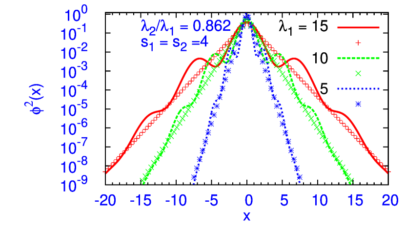
Figure 1: (Color online) Numerical density $\phi^{2}(x)$ (line) and its exponential fit (symbol) vs. $x$ for $\lambda_{1}=15,10$ and 5.

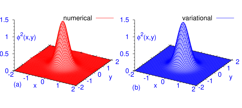
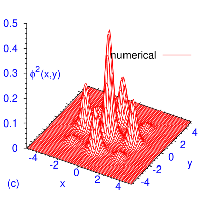
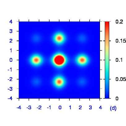
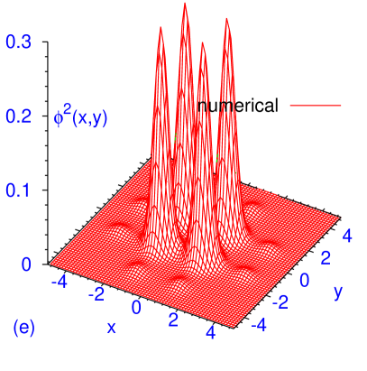
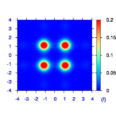
Figure 2: (Color online) (a) Numerical and (b) variational density $\phi^{2}(x,y)$ vs. $x$ and $y$ from a solution of Eqs. (8) and (6) for a disk-shaped BEC for $g=0$. (c) Numerical density $\phi^{2}(x,y)$ vs. $x$ and $y$ and (d) its contour plot from a solution of Eqs. (8) and (6) for a disk-shaped BEC for $g=2$. (e) Numerical density $\phi^{2}(x,y)$ vs. $x$ and $y$ and (f) its contour plot from a solution of Eqs. (8) and (5) for a disk-shaped BEC for $g=2$. Quantities $\phi^{2}(x,y)$ and $x,y$ are all in dimensionless harmonic oscillator units.

III.1 2D Bichromatic Optical Lattice

To study the localization of a BEC in 2D and 3D with potentials (5) and (6), we set the ratio $\lambda_{2}/\lambda_{1}=0.86$ (roughly the same ratio $\lambda_{2}/\lambda_{1}$ as in the experiment of Roati et al. roati ). First we consider the solution of Eq. (8) for a disk-shaped BEC. To understand the nature of these localized states, we consider the localized states with larger values of $\lambda_{1}$. Such states with a large $s_{2}/s_{1}(=1)$ occupy a small number of OL sites and hence their numerical simulation can be performed relatively easily. All results reported in Secs. III.1 and III.2 are obtained with the following parameters in the bichromatic OL potentials (5) and (6): $\lambda_{1}=5,$ $\lambda_{2}/\lambda_{1}=0.86,$ and $s_{1}=s_{2}=4$. It now remains to be seen if with this set of parameters the localized state is in the limit of weak disorder with an exponential tail. In 1D this would mean $\phi(x)\sim\exp(-x/L_{\mathrm{loc}})$, where $L_{\mathrm{loc}}$ is the localization length. In Fig. 1 we plotted the numerical probability $\phi^{2}(x)$ vs. $x$ on a log scale, together with a fitting exponential function with $L_{\mathrm{loc}}=0.75,1.5$ and 2.2, respectively, for $\lambda_{1}=5,10$ and 15. These localization lengths are large compared to the root mean square (rms) size of the localized states, which are 0.53, 1.05, and 1.55 for $\lambda_{1}=5,10$ and 15. The wave functions shown in Fig. 1 are identical to those shown in Fig. 1 (a) of Ref. adhikari where the central part of these wave functions are well fitted to Gaussian variational approximations.

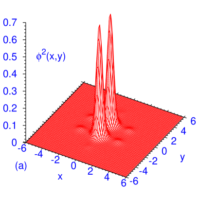
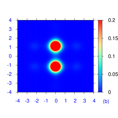
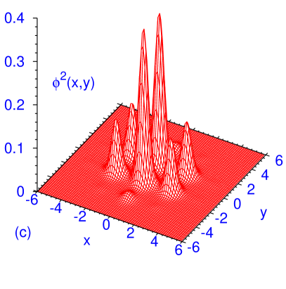
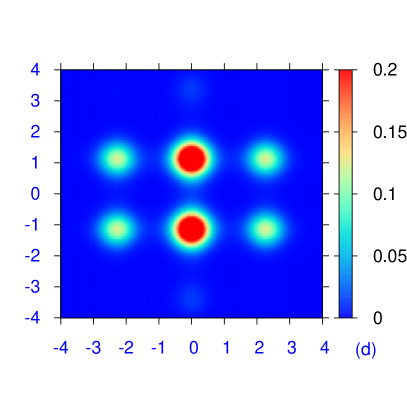
Figure 3: (Color online) (a) Density $\phi^{2}(x,y)$ of a disk-shaped BEC from a numerical solution of Eq. (8) with (b) its contour plot for potential (6) along $x$ direction and potential (5) along $y$ direction for $g=0$. (c) Same as (a) but with $g=2$. (d) Same as (b) but with $g=2.$ All quantities are in oscillator units.

In Figs. 2 (a) and (b) we plot the results for density $\phi^{2}(x,y)$ vs. $x$ and $y$ from numerical and variational solutions of Eqs. (8) and (6) for $g=0$, respectively. (The $g=0$ case is trivial as the 2D and 3D Eqs. (8) and (4) decouple into two and three 1D equations, respectively. Nevertheless, this case allows us to test carefully the numerical programs by comparing the variational result with the two numerical results obtained by real- and imaginary-time propagation.) The variational width ($w=0.4864$) obtained from a solution of Eq. (13) produced the density in good agreement with the numerical density in Fig. 2 (a). In Fig. 2 (c) we plot the results for density $\phi^{2}(x,y)$ vs. $x$ and $y$ from a numerical solution of Eqs. (8) and (6) for the same set of parameters as in Fig. 2 (a) but with $g=2$. (As in 1D adhikari ; modugno2 , repulsive nonlinearity $g$ has a strong effect on localization. As $g$ is increased to a small positive value, the localized states occupy more and more lattice sites with larger spatial extension.) In Fig. 2 (d) we show a contour plot of the density shown in Fig. 2 (c). Because of the nonlinear inter-atomic repulsion, the essentially single peak of Fig. 2 (a) now transforms into a multi-peak structure, although the central peak is still the strongest. Finally, in Figs. 2 (e) and (f) we plot $\phi^{2}(x,y)$ vs. $x$ and $y$ and its contour plot from a numerical solution of Eqs. (8) and (5) for $g=2$. Due to a change in the nature of the potential from Eq. (6) (sine, minimum of potential at origin) to Eq. (5) (cosine, maximum of potential at origin) the central region has a minimum of density in this case and not a maximum as in Figs. 2 (a) and (c). The difference in the structure of the BEC densities can clearly be seen from the respective contour plots.

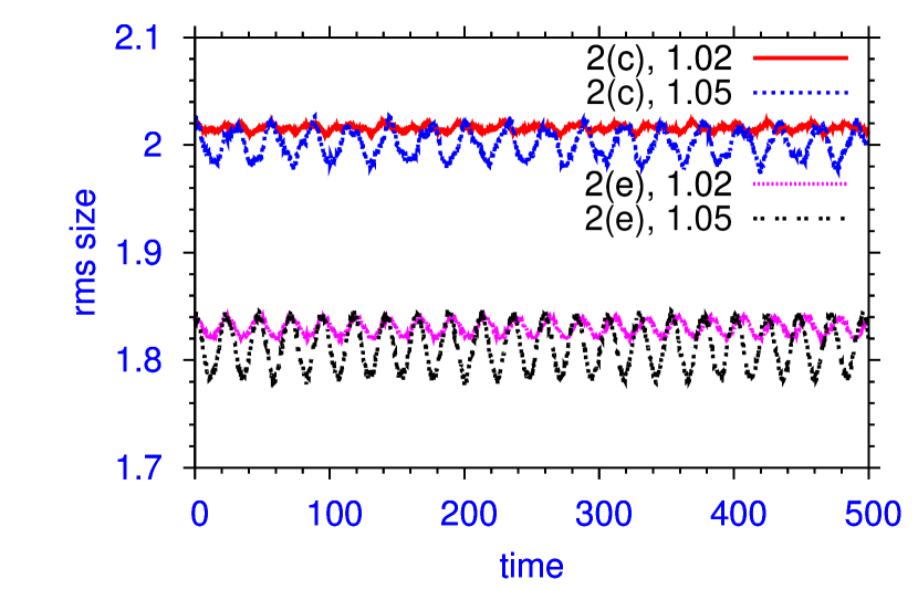
Figure 4: (Color online) Time evolution of the rms sizes of the BECs depicted in Figs. 2 (c) and (e) as the potential is multiplied suddenly by a factor of 1.02 or 1.05. All quantities are in oscillator units.

We also calculated the chemical potential of the states illustrated in Figs. 2. The numerical result for energy for potential (6) of Fig. 2 (a) is 4.747, to be compared with the variational result of Eq. (14) 4.791, calculated with width $w=0.4864$ obtained by solving Eq. (13). This agreement between the numerical and variational results of the BEC density for potential (6) in Fig. 2 (a), and of the respective energies, provides assurance about the accuracy of the numerical code used in simulation in our investigation. We also calculated the (numerical) chemical potential of the BEC density displayed in Figs. 2 (c) ($\mu=5.102$) and (e) ($\mu=5.103$). The two chemical potentials are practically the same. A similar finding was noted in the 1D case as the potential was changed from sine to cosine type adhikari .

As we are considering two potentials (5) and (6) in 2D and 3D it is possible to have a distinct potential along each axis. We consider this possibility in the case of the localized state in a disk-shaped BEC where we take potential (5) along $x$ direction and potential (6) along $y$ direction with $g=0$. The density and the contour plot of the BEC in this case are shown in Figs. 3 (a) and (b). Just to illustrate the effect of a small nonlinearity on the localized state we repeated the numerical simulation in this case with a nonlinearity $g=2$. The density and the corresponding contour plot of the resulting localized state are shown in Figs. 3 (c) and (d). The density in Fig. 3 (c) is quite similar to that in Fig. 3 (a), with the exception that the density in Fig. 3 (c) extends over more sites due to the repulsive nonlinearity.

Next we explicitly demonstrate that the densities shown in Figs. 2 corresponds to stable states. For this we consider the time evolution of the BECs illustrated in Figs. 2 (c) and (e) in a slightly altered potential, e.g., the potential obtained by multiplying the original potentials by a factor of 1.02 and 1.05. The resultant rms sizes as calculated by the real-time propagation routine are plotted in Fig. 4. The curves in Fig. 4 are labeled by Fig. 2 (c) or (e) and the factor 1.02 or 1.05 which multiplies the potential. In all cases the rms sizes execute breathing oscillation over a long period of time as shown in Fig. 4 and this demonstrates the stability of the localized states.

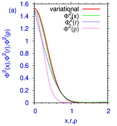
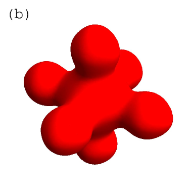
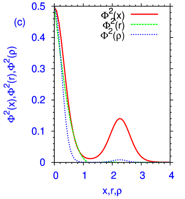
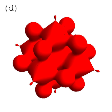
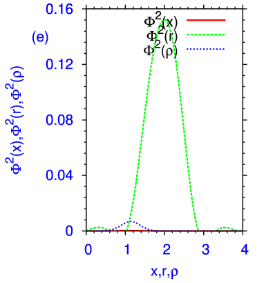
Figure 5: (Color online) (a) Sections of density $\phi^{2}(x,y,z)$ for a 3D BEC from a solution of Eq. (4) with the (b) 3D contour plot of density $\phi^{2}(x,y,z)$ for potential (6) with $g=0$; (c) Same as (a) with $g=2$; (d) Same as (b) with $g=2$; (e) Same as (a) with potential (5) with the parameters $\lambda_{1}=5,\lambda_{2}/\lambda_{1}=0.86,s_{1}=s_{2}=4$ and $g=2$; (f) Contour plot for (e). The sections plotted in the left panel are $\Phi^{2}(x)\equiv\phi^{2}(x,0,0)$ vs. $x$, $\Phi^{2}(\rho)\equiv\phi^{2}(0,\rho/\sqrt{2},\rho/\sqrt{2})$ vs. $\rho$, and $\Phi^{2}(r)\equiv\phi^{2}(r/\sqrt{3},r/\sqrt{3},r/\sqrt{3})$ vs. $r$. For potential (6) the variational result for $\Phi^{2}(r)$ vs. $r$ is also plotted.

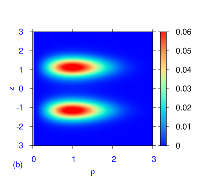
Figure 6: (Color online) (a) 2D contour plot of the BEC density $\phi^{2}(\rho,z)$ for a localized 3D vortex in bichromatic OL potential (6) with $g=5$, obtained by solving Eq. (II). The vortex core appears as the line $\rho=0$. (b) Same as (a) in bichromatic OL potential (5). As potential (5) has a maximum at $z=0$ the matter density is zero there.

III.2 3D Bichromatic Optical Lattice

Now we consider a few cases of the localized states in 3D as obtained from a solution of Eq. (4) together with potential (5) or (6) along three orthogonal directions. First, as in 2D, we consider the solution of Eq. (4) with potential (6) for $g=0$. The result is illustrated in Figs. 5 (a) and (b). In Fig. 5 (a) we plot three sections of the density $-$ $\Phi^{2}(x)\equiv\phi^{2}(x,0,0)$ vs. $x$, $\Phi^{2}(r)\equiv\phi^{2}(r/\sqrt{3},r/\sqrt{3},r/\sqrt{3})$ vs. $r$, and $\Phi^{2}(\rho)\equiv\phi^{2}(0,\rho/\sqrt{2},\rho/\sqrt{2})$ vs. $\rho$ $-$ together with the variational result. Here $\Phi^{2}(x)$ corresponds to the density in the axial $x$ direction with polar angle $\theta=0$, $\Phi^{2}(r)$ that in the diagonal direction with polar angle $\theta=\pi/4$ and azimuthal angle $\varphi=\pi/4$, and $\Phi^{2}(\rho)$ that in the transverse direction with polar angle $\theta=\pi/2$ and azimuthal angle $\varphi=\pi/4$. In Fig. 5 (b) we show the 3D contour plot (obtained using Mathematica) of the BEC density showing the actual shape of the localized state. (The value of the density at the boundary of the plot is 0.001 in Figs. 5 (b), (d) and (f).) As $g=0$ in Fig. 5 (a), the 3D wave function is trivial and decouples in the three directions. The variational result in this case is in good agreement with the numerical result for the density in the diagonal direction $-$ $\Phi^{2}(r)$. Next we consider the nontrivial 3D case with $g=2$ for potential (6). In this case the 3D solution has no 1D counterpart. In Figs. 5 (c) and (d) we plot the sections of the densities and the 3D contour plot, respectively, for potential (6) with $g=2$. The shape of the BEC density is similar to the $g=0$ case with a maximum at the origin, the only difference being that in Fig. 5 (c) the density extends over a larger distance in space due to the repulsion introduced by a positive $g$ value. The density has secondary maxima in adjacent OL sites in this case. Finally, in Fig. 5 (e) and (f) we show the results for the density and its 3D contour plot, respectively, with potential (5) and $g=2$. Now the density has a minimum at the origin in contrast to the maxima in Figs. 5 (a) and (c). Also, in Figs. 5 (e) and (f) the density is zero along the three axes (explicitly shown in $x$ direction with $\Phi^{2}(x)=0$).

Next we consider the localization in a 3D bichromatic OL potential of a noninteracting BEC vortex with $g=5$ rotating around the $z$ direction with unit angular momentum from a numerical solution of Eq. (II). In this case we consider potentials (6) and (5) along the $z$ direction. For a localized 3D vortex state rotating around the $z$ direction and described by Eq. (II) under the action of the bichromatic OL potentials (6) and (5), a vortex core of zero density passing through the origin develops along the $z$ axis. To illustrate the vortex state we solve Eq. (II) with potentials (6) and (5) for $g=5.$ In Figs. 6 (a) and (b) we show the contour plot of the density $\phi(\rho,z)$ for potentials (6) and (5), respectively. For potential (5), in addition to the vortex core along the $z$ axis, the density is also zero along the $z=0$ line.

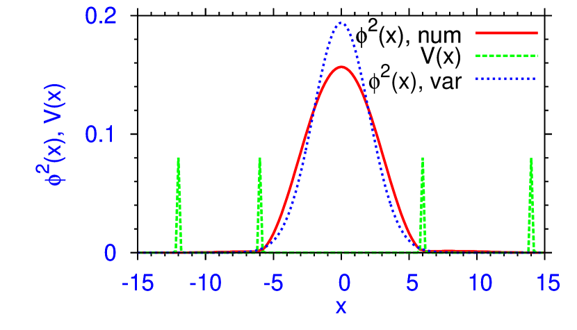
Figure 7: (Color online) The numerical (num) and variational (var) BEC density $\phi^{2}(x)$ vs. $x$ for the random potential (15) with $B_{i}=8,c_{i}=100,x_{10}=-12,x_{20}=-6,x_{30}=6,x_{40}=14$ and $g=0$. The potential $V(x)$ is also plotted in arbitrary units.

III.3 Random Spike Potential

Now we consider the localization of a BEC in the 1D random potential (15). For small values of the amplitude $B_{i}$, a large number $S$ of spikes is needed for a good localization. However we consider the minimum number $S(=4)$ of spikes for localization. For a robust localization with $S=4$, we take $B_{i}=8$ and $c_{i}=100$ corresponding to a Gaussian spike of very small width. Next we had to choose the random positions $\beta_{i}$. Different sets of unevenly distributed $\beta_{i}$ produced localization and here we take $\beta_{i}=-12,-6,6,14$ for $i=1,2,3,4$. This choice of the points sets the center of the localized BEC approximately at $x=0$. In Fig. 7 we plot the localized BEC density $\phi^{2}(x)$ vs. $x$ for nonlinearity $g=0$. The variational and numerical chemical potentials are 0.03739 and 0.03093, respectively. The plot of the potential (in arbitrary units) is also shown in Fig. 7. With this potential the localization is destroyed for a very small nonlinearity $g(\sim 1)$, unless the number of spikes is increased and we do not consider the localization of an interacting BEC here.

IV SUMMARY

In this paper, using the numerical solution CPC of the GP equation GP in 2D and 3D, we studied the localization roati ; billy of a noninteracting and weakly interacting BEC in a quasi-periodic bichromatic OL potential along different axes. We considered two analytical forms (sine and cosine) of the OL potential, e.g., (5) and (6) and considered the same or different potentials along different axes. First we consider the localization of a disk-shaped BEC with a small repulsive nonlinearity under the action of the bichromatic OL potential (5) or (6). We considered the localization of a full 3D BEC under the action of bichromatic OL potentials (5) or (6) along the three axes with or without a small nonlinear atomic interaction. The increase of nonlinearity destroys localization in all cases considered adhikari ; dnlse ; modugno2 . We also considered the localization of a noninteracting BEC vortex of unit angular momentum with a 3D bichromatic OL potential (6) or (5) along the axial direction and harmonic traps along the transverse radial directions. The clear stable vortex cores in 3D as shown in Figs. 6 (a) and (b) are the most important findings of this paper. Finally, we showed that one can have localized noninteracting BEC states under the action of random potentials taken in the form of repulsive spikes randomly distributed in space. All these localized states are found to be dynamically stable.

We hope that the present work will motivate new studies, specially experimental ones, on localization in a more realistic 2D and 3D BEC under the action of bichromatic OL potentials along different axes. Specially challenging is the localization of a singly-quantized vortex BEC in 3D as predicted in this work. The consideration of a vortex lattice of BEC ketterle in bichromatic OL potentials is of great interest also. It remains to be seen if one has vortex pinning in a rotating BEC as observed in a monochromatic OL potential superposed on a harmonic trap cornell . The effect of a bichromatic OL potential on a two-species mixture of BECs two is also of interest. In the bichromatic OL potential considered in this paper, the disorder term is taken in the form of a periodic potential with an incommensurate wave length. We also considered a disordered potential in the form of narrow identical repulsive spikes distributed randomly in space. Further work need be done to study the effect of different types disorder terms. The 2D and 3D localization of BEC under the action of bichromatic OL potentials and of a random potential $-$ as predicted in this paper $-$ may find application in other contexts in 2D and 3D, for example, in the localization of electron waves in 2D and 3D lattice as well as in the localization of electromagnetic waves, or sound waves in the presence of disorder.

- (1) P. W. Anderson, Phys. Rev. 109, 1492 (1958).
- (2) D. S. Wiersma et al., Nature 390, 671 (1997); F. Scheffold et al., ibid. 398, 206 (1999).
- (3) R. Dalichaouch et al., Nature 354, 53 (1991); A. A. Chabanov et al., ibid. 404, 850 (2000).
- (4) R. L. Weaver et al., Wave Motion 12, 129 (1990).
- (5) J. Billy et al., Nature 453, 891 (2008).
- (6) G. Roati et al., Nature 453, 895 (2008).
- (7) J. Chabé et al., Phys. Rev. Lett. 101, 255702 (2008).
- (8) E. E. Edwards, M. Beeler, T. Hong, and S. L. Rolston, Phys. Rev. Lett. 101, 260402 (2008).
- (9) L. Pitaevskii and S. Stringari, Bose Einstein Condensation (Oxford University Press, Oxford, 2003).
- (10) C. J. Pethick and H. Smith, Bose Einstein Condensation in Dilute Gases (Cambridge University Press, Cambridge, England, 2002).
- (11) S. Inouye, M. R. Andrews, J. Stenger et al., Nature 392, 151 (1998).
- (12) P. G. Harper, Proc. Phys. Soc. Lond. A 68, 874 (1955).
- (13) D. J. Boers, B. Goedeke, D. Hinrichs, and M. Holthaus, Phys. Rev. A 75, 063404 (2007).
- (14) S. Aubry and G. André, Ann. Isr. Phys. Soc. 3, 133 (1980); G. Kopidakis, S. Komineas, S. Flach, and S. Aubry, Phys. Rev. Lett. 100, 084103 (2008).
- (15) D. J. Thouless, Phys. Rev. B 28, 4272 (1983).
- (16) L. Sanchez-Palencia et al., Phys. Rev. Lett. 98, 210401 (2007); D. Clément et al., ibid. 95, 170409 (2005); J. E. Lye et al., Phys. Rev. Lett. 95, 070401 (2005).
- (17) B. Damski, J. Zakrzewski, L. Santos, P. Zoller, and M. Lewenstein, Phys. Rev. Lett. 91, 080403 (2003); T. Schulte et al., ibid. 95, 170411 (2005).
- (18) M. Modugno, New. J. Phys. 11, 033023 (2009).
- (19) M. Larcher, F. Dalfovo, and M. Modugno, Phys. Rev. A 80, 053606 (2009).
- (20) S. K. Adhikari and L. Salasnich, Phys. Rev. A 80, 023606 (2009).
- (21) G. Roux et al., Phys. Rev. A 78, 023628 (2008).
- (22) T. Roscilde, Phys. Rev. A 77, 063605 (2008); X. Deng, R. Citro, E. Orignac, and A. Minguzzi, Eur. Phys. J. B 68, 435 (2009).
- (23) T. Paul, M. Albert, P. Schlagheck, P. Leboeuf, and N. Pavloff, Phys. Rev. A 80, 033615 (2009).
- (24) A. S. Pikovsky and D. L. Shepelyansky, Phys. Rev. Lett. 100, 094101 (2008); S. Flach, D. O. Krimer, and Ch. Skokos, Phys. Rev. Lett. 102, 024101 (2009), I. García-Mata and D. L. Shepelyansky, Phys. Rev. E 79, 026205 (2009); Ch. Skokos, D. O. Krimer, S. Komineas, and S. Flach, Phys. Rev. E 79, 056211 (2009).
- (25) J. Biddle, B. Wang, D. J. Priour, Jr., and S. Das Sarma, Physical Review A 80, 021603(R) (2009).
- (26) E. P. Gross, Nuovo Cimento 20, 454 (1961); L. P. Pitaevskii, Zh. Eksp. Teor. Fiz. 40, 646 (1961) [Sov. Phys. JETP 13, 451 (1961)].
- (27) T. Schwartz et al., Nature 446, 52 (2007); Y. Lahini et al., Phys. Rev. Lett. 100, 013906 (2008); Y. Lahini et al., Phys. Rev. Lett. 103, 013901 (2009).
- (28) W. Hänsel, P. Hommelhoff, T. W. Hänsch, and J. Reichel Nature (London) 413, 498 (2001).
- (29) Y. Shin et al., Phys. Rev. A 72, 021604(R) (2005); T. Schumm et al., Nature Physics 1, 57 (2005); J. Estève et al., Eur. Phys. J. D 35, 141 (2005).
- (30) A. Wobst, G. L. Ingold, P. Hanggi, and D. Weinmann, Phys. Rev. B 68, 085103 (2003).
- (31) G. Srinivasan, A. Aceves, and D. M. Tartakovsky, Phys. Rev. A 77, 063806 (2008).
- (32) C. Fort et al., Phys. Rev. Lett. 95, 170410 (2005); D. R. Grempel, S. Fishman, and R. E. Prange, ibid. 49, 833 (1982); L. Fallani, J. E. Lye, V. Guarrera, C. Fort, and M. Inguscio, ibid. 98, 130404 (2007); P. Lugan, D. Clement, P. Bouyer, A. Aspect, M. Lewenstein, and L. Sanchez-Palencia, ibid. 98, 170403 (2007); N. Bilas and N. Pavloff, Eur. Phys. J. D 40, 387 (2006); C. Tang and M. Kohmoto, Phys. Rev. B 34, 2041 (1986).
- (33) P. Lugan, D. Clement, P. Bouyer, A. Aspect, and L. Sanchez-Palencia, Phys. Rev. Lett. 99, 180402 (2007); J. E. Lye et al., Phys. Rev. A 75, 061603(R) (2007).
- (34) R. C. Kuhn, C. Miniatura, D. Delande, O. Sigwarth, and C. A. Muller, Phys. Rev. Lett. 95, 250403 (2005); S. E. Skipetrov, A. Minguzzi, B. A. vanTiggelen, and B. Shapiro, ibid. 100, 165301 (2008); E. Abrahams, P. W. Anderson, D. C. Licciardello, and T. V. Ramakrishnan, ibid. 42, 673 (1979).
- (35) S. K. Adhikari and B. A. Malomed, Phys. Rev. A 79, 015602 (2009); 76, 043626 (2007); Europhys. Lett. 79, 50003 (2007); Physica D 238, 1402 (2009).
- (36) F. Dalfovo and S. Stringari, Phys. Rev. A 53, 2477 (1996).
- (37) S. K. Adhikari, Am. J. Phys. 54, 362 (1986).
- (38) P. Muruganandam and S. K. Adhikari, Comput. Phys. Commun. 180, 1888 (2009).
- (39) V. M. Pérez-García, H. Michinel, J. I. Cirac, M. Lewenstein, and P. Zoller, Phys. Rev. A 56, 1424 (1997).
- (40) P. Muruganandam and S. K. Adhikari, J. Phys. B 36, 2501 (2003); S. K. Adhikari and P. Muruganandam, J. Phys. B 35, 2831 (2002); S. K. Adhikari, Phys. Rev. E 62, 2937 (2000); Phys. Lett. A 265, 91 (2000).
- (41) A. Soibel, E. Zeldov, M. Rappaport et al., Nature 406, 282 (2000); J. R. Abo-Shaeer, C. Raman, J. M. Vogels, and W. Ketterle, Science 292, 476 (2001).
- (42) S. Tung, V. Schweikhard, and E. A. Cornell, Phys. Rev. Lett. 97, 240402 (2006).
- (43) S. K. Adhikari, Phys. Lett. A 346, 179 (2005); V. M. Pérez-García and J. B. Beitia, Phys. Rev. A 72, 033620 (2005).