Scaling laws of resistive magnetohydrodynamic reconnection in the high-Lundquist-number, plasmoid-unstable regime
Abstract
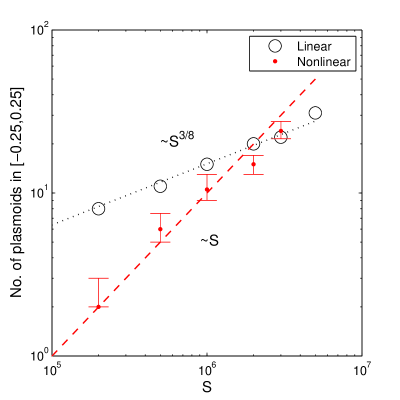
The Sweet-Parker layer in a system that exceeds a critical value of the Lundquist number () is unstable to the plasmoid instability. In this paper, a numerical scaling study has been done with an island coalescing system driven by a low level of random noise. In the early stage, a primary Sweet-Parker layer forms between the two coalescing islands. The primary Sweet-Parker layer breaks into multiple plasmoids and even thinner current sheets through multiple levels of cascading if the Lundquist number is greater than a critical value . As a result of the plasmoid instability, the system realizes a fast nonlinear reconnection rate that is nearly independent of , and is only weakly dependent on the level of noise. The number of plasmoids in the linear regime is found to scales as , as predicted by an earlier asymptotic analysis (Loureiro et al., Phys. Plasmas 14, 100703 (2007)). In the nonlinear regime, the number of plasmoids follows a steeper scaling, and is proportional to . The thickness and length of current sheets are found to scale as , and the local current densities of current sheets scale as . Heuristic arguments are given in support of theses scaling relations.
I Introduction
Recent studies of nonlinear reconnection in large high-Lundquist-number () plasmas, based on resistive magnetohydrodynamics (MHD) Bhattacharjee et al. (2009) as well as fully kinetic simulations that include a collision operator Daughton et al. (2009) have produced a surprise. It is seen in these studies that above a critical value of the Lundquist number, the system deviates qualitatively from the predictions of Sweet-Parker theory Sweet (1958); Parker (1963) which has been the standard model for reconnection in the high- regime. In the Sweet-Parker model, the reconnection layer has the structure of Y-points, with a length of the order of the system size, and a width given by , where is the Lundquist number based on the system size , the Alfvén speed , and the magnetic diffusivity . The Sweet-Parker model is usually considered to be a model of “slow” reconnection as it predicts the reconnection rate to scale as . (The Petschek model Petschek (1964) predicts a much weaker dependence on , with the maximum reconnection rate . However, it has become clear over the years that Petschek model is realizable only when the resistivity is locally enhanced around the reconnection site. Biskamp (2000)) For weakly collisional systems such as the solar corona, the Lundquist number is typically very large () and the Sweet-Parker reconnection time scale is of the order of years, much too slow to account for fast events such as solar flares. The Sweet-Parker model is based on the assumption of the existence of a long thin current layer. Although it has been known for some time that such a thin current layer may be unstable to a secondary tearing instability (referred to hereafter as the plasmoid instability) which generates plasmoids,Bulanov et al. (1979); Lee and Fu (1986); Biskamp (1986); Yan et al. (1992); Shibata and Tanuma (2001); Lapenta (2008) it has been realized only fairly recently that the Sweet-Parker layer actually becomes more unstable as the Lundquist number increases, with a linear growth rate and the number of plasmoids .Loureiro et al. (2007); Bhattacharjee et al. (2009) In a recent paper (Ref. Bhattacharjee et al. (2009), hereafter referred to as Paper I), Bhattacharjee et al. have presented numerical results that suggest strongly that as a consequence of the plasmoid instability, the system evolves into a nonlinear regime in which the reconnection rate becomes weakly dependent on .
The primary goal of this paper is to strengthen the results obtained in Paper I in two significant ways: first, to present new simulation results with a modified initial condition that enables us to obtain stronger scaling results on the nonlinear reconnection rate and the number of plasmoids generated in the nonlinear regime, and second, a simple heuristic model that is consistent with the results of the simulation and fortifies the claim in Paper I that the reconnection rate in the nonlinear regime of the plasmoid instability is fast and independent of .
II Numerical Model
The initial condition in Paper I does not have a thin current sheet to begin with. It has four magnetic islands and is unstable to an ideal coalescence instability. After the onset of the coalescence instability, a Sweet-Parker current sheet is created when two islands are attracted toward each other.Longcope and Strauss (1993) In this case, there is a relatively long initial transient period before the reconnection process starts. Furthermore, the dynamics of the system are complicated by the sloshing of coalescing islands that causes the primary Sweet-Parker layer to lengthen or shorten from time to time. This makes it difficult to verify the predictions of linear theory in this particular system. The present study seeks remedies to these two drawbacks. We still consider the merging of two islands, but now put them in close contact initially. There is an initial current layer between the flux tubes, which quickly (typically within less than one Alfvén time) adjusts its width depending on the Lundquist number to form the primary Sweet-Parker layer, which may subsequently become unstable to the plasmoid instability. In this new system, the transient period is significantly shortened and the sloshing between islands is largely eliminated. It is still not easy to measure the linear growth rate in this new model, but we can at least verify the scaling of the number of plasmoids in the linear regime.
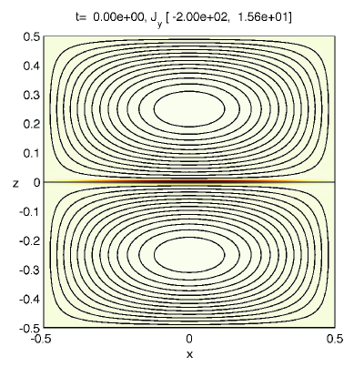
The initial condition is similar to the model of Uzdensky and Kulsrud.Uzdensky and Kulsrud (2000) To start with, let and in the domain . The so defined satisfies . If the pressure is set to with an arbitrary constant, the system is in force balance. However, the magnetic field defined by has a tangential discontinuity at , which causes numerical difficulties. We smooth it out as where is a large number. This smoothed function no longer satisfies and the magnetic force cannot be balanced entirely by pressure. However, the magnetic force can be canceled to a large extent if the pressure is set to , where and , respectively. We assume the isothermal equation of state, , in our simulation. We choose , , and . For these parameters, the initial plasma density varies from to and the plasma beta () obeys the inequality . The system is, therefore, nearly incompressible. Figure 1 shows the initial current density and magnetic field lines.
We find in the present study that the plasmoid instability depends on the noise level of the system, at least when the Lundquist number is not far above the critical value. Due to the outflow in the primary Sweet-Parker layer, if the noise level is low, the plasmoid instability may not grow to visible size before being convected out. When we seed the system initially with random noise, at relatively low values of the Lundquist number () we obtain a short burst of plasmoids, following which the current layer becomes stable again after all the plasmoids are convected out. Because of this, we have included a random forcing in the system, which enables us also to study the effect of noise level on the reconnection rate. (Notice that we did not apply any random forcing or noise in Paper I. The sloshing between coalescing islands is a natural source of noise, but uncontrolled.) The governing equations for the time evolution of the system are:
| (1) |
| (2) |
| (3) |
where a random forcing term is added to the right hand side of the momentum equation (2). The forcing function is white noise in both space and time with , and is a small parameter which controls the noise level. By white noise we mean that where and can be or and is the ensemble average. Care has to be taken to ensure that the discrete representation is independent of the time step. Our implementation is similar to that in Ref.Alvelius (1999). It is convenient to set , where is a random acceleration. In a single time step, the momentum density evolves from to (neglecting other forces), and the kinetic energy density evolves from to . Therefore, the average power density from the random force is
where is used, and . At each grid point, we set , to random numbers between and with a uniform probability distribution, divided by . That is,
Then and is independent of . The average power density is and the total power with the total mass ( in our simulation). We use in our simulations and the corresponding power density ranges from to . Since our simulations typically last only a few Alfvén times, the energy input from random forcing is negligible compared to the total magnetic energy () in the system. This ensures that the random forcing only provides noise for the instability to grow but does not otherwise alter the system in a significant way (see more discussion in Sec. III).
Our numerical algorithm Guzdar et al. (1993) uses finite differences with a five-point stencil in each direction, and a second-order accurate trapezoidal leapfrog method for time stepping. We use a uniform grid along the direction, and a nonuniform grid in the direction that packs high resolution around in order to resolve the sharp spatial gradients in the reconnection layer. Perfectly conducting (), impenetrable (), and free slipping () boundary conditions are assumed ( is the unit normal vector to the boundary). We further assume reflection symmetry along the axis and only the region is simulated. The highest resolution is in and in , with the smallest grid size .
III Numerical Results
One of the key objectives of this study is to determine the scaling of reconnection rate in the plasmoid-unstable regime. To quantify the speed of reconnection, we measure the time it takes to reconnect a significant portion of the magnetic flux within the two merging islands. The amount of magnetic flux in an island is , where is the maximum of in the island and is the value of at the separatrix separating the two merging islands. Initially and it remains approximately unchanged since the resistivity is low; therefore it suffices to just measure . We denote the time it takes to reconnect from to as . The starting point is chosen to allow the plasmoid instability to build up, and the end point is chosen such that the reconnection layer does not shorten too much compared with that in the initial condition. The range corresponds to reconnecting of the initial flux.
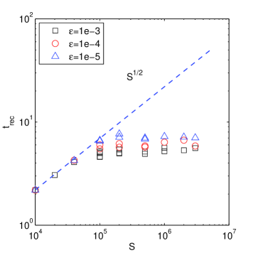
Figure 2 shows the reconnection time for various and . For lower , the reconnection time , as expected from the Sweet-Parker theory.Uzdensky and Kulsrud (2000) The critical Lundquist number for plasmoid instability is about . Above , the reconnection time deviates from the Sweet-Parker scaling and becomes shorter. In the plasmoid unstable regime, the reconnection time is nearly independent of . However, the reconnection time has a weak dependence on the noise level throughout the range we have tested. The plateaued values of in the high- regimes for , , and are , , and , respectively. Here we take the average values over the range to , and the errors represent the standard deviation. We have tested the convergence of our numerical results by varying the resolution, the time step, and the random seed for selected runs. These are represented by multiple data points with the same parameters in Figure 2. The results are fairly consistent, with fluctuations no more than a few percent. The dependence of on may be tentatively fit with a power law, which gives . However, given the limited range of the parameter space we have explored, this scaling should not be considered as conclusive.
The global characteristic values for and are about , which yield the normalized average reconnection rate as
In the high Lundquist number regime, to from our simulations and the normalized reconnection rate is in the range to . The normalized reconnection rate obtained here is similar to the result of Paper I.
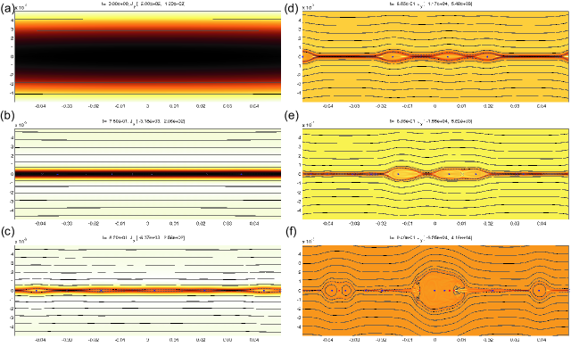
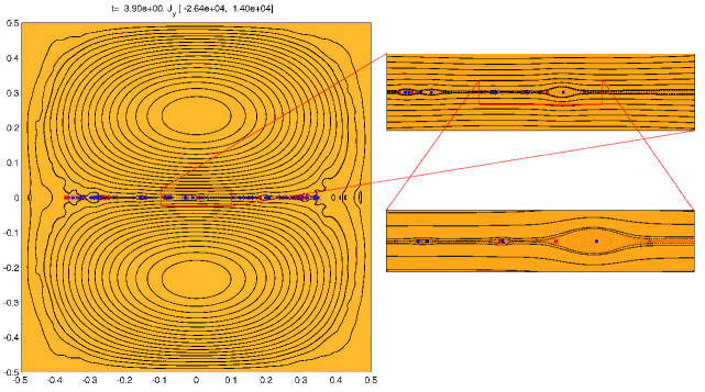
Figure 3 shows a time sequence of the current density, overlaid with magnetic field lines, within a small area () of the whole domain for a case with and . The initial current layer (panel (a)) quickly thins down to form the primary Sweet-Parker layer (panel(b)), which becomes unstable to the plasmoid instability (panel (c)). As the instability proceeds, the plasmoids grow in size and the current sheets between plasmoids are again Sweet-Parker like (panel (d)). These secondary Sweet-Parker current sheets are thinner than the primary one and are again unstable to the tertiary plasmoid instability (panel (e)). This process of multiple stages of cascading resembles the scenario envisaged in Ref.Shibata and Tanuma (2001). The plasmoids can merge to form larger ones and new plasmoids are constantly generated (panel (f)). Figure 4 shows the global configuration at a later time , as well as close-ups of the reconnection layer. The figure shows that on a large, coarse-grained scale, the configuration looks Sweet-Parker like, except for the important difference that the reconnection layer is no longer a single extended current sheet, but is made up of a sequence of copious plasmoids and current sheets.
Linear theory predicts that the number of plasmoids, , scales as .Loureiro et al. (2007); Bhattacharjee et al. (2009) We verify this by counting the maximum number of plasmoids within the central region, , before the plasmoid instability becomes highly nonlinear (roughly corresponds to panel (c) in Figure 3). Figure 5 shows the number of plasmoids versus , for , in both linear and nonlinear (see the discussion later) regimes. The result in the linear regime is in good agreement with the scaling predicted by asymptotic analysis. This scaling has been verified by Samtaney et al. with local simulations up to .Samtaney et al. (2009)
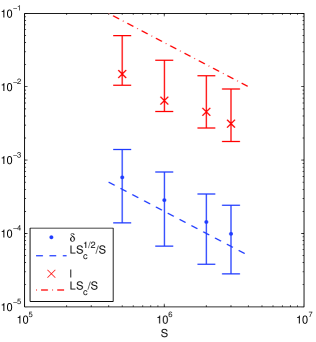
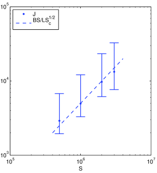
In the fully nonlinear regime, the plasmoid dynamics are very complicated and constantly evolving. Plasmoids may grow in size, coalesce with each other to form larger plasmoids, and finally get ejected into the downstream region. Meanwhile, new plasmoids are constantly generated in the reconnection layer. We may regard the reconnection layer with multiple plasmoids as a statistical steady state. As a simple, first approximation, we expect the cascading to stop when the current sheet segments between plasmoids become stable. We may imagine the reconnection layer as a chain of plasmoids connected by marginally stable Sweet-Parker current sheets. For given and , the critical length of a marginally stable current layer is . Therefore we expect the number of plasmoids in the nonlinear regime, , to scale like . Furthermore, the thickness of each Sweet-Parker sheet is , and the current density . If we identify the reconnection rate with , then the reconnection rate , which is independent of . This is consistent with our finding that the reconnection rate is nearly independent of in the high- regime. Clearly, the assumption that all current sheets are marginally stable, and therefore all identical, is oversimplified. If we look at the individual current sheets, there are a whole variety of them, each with a different length, width, and current density. Therefore, the system is better described with a statistical approach. If we neglect complications such as asymmetry or background shear flow, and consider the simple Sweet-Parker picture for each current sheet, then the local Lundquist number is the only dimensionless parameter associated with it. Here denotes the length of the current sheet. The current sheet thickness will be , as predicted by the Sweet-Parker theory. The local Lundquist number being greater or smaller than determines whether a current sheet may or may not further break into plasmoids and even smaller current sheets. Because it is the local Lundquist number that determines the cascading of a local current sheet to even smaller scales, we hypothesize that the probability distribution of is independent of the global Lundquist number. The underlying assumption is that, if we consider the ensemble of local current sheets and characterize each current sheet by a dimensionless parameter , there is a similarity across systems of different global Lundquist numbers. If we further assume that the local upstream Alfvén speed is determined by global conditions, it follows that statistically the length and the thickness of a current sheet scale as , and the current density scales as . If we consider the simple picture that two neighboring current sheets are separated by a plasmoid, then implies the number of plasmoids in the nonlinear regime .
Now we proceed to examine whether the conclusions from the simple heuristic argument are consistent with our simulation data. Here we present the results from cases with . Results from other values of are similar. We count the number of plasmoids by first identifying X-points and O-points along . There are two types of O-points, the local minimum (type I) and the local maximum (type II) of . Likewise, there are two types of X-points, one with , (type I) and the other with , (type II). In the linear regime, only X-points and O-points of type I are present. When plasmoids start to coalesce with each other, type II null points may be created. We count the number of type I O-points within as the number of plasmoids in the nonlinear regime. As shown in Figure 5, the number of plasmoids in the nonlinear regime appears to agree with the scaling. Because the number of plasmoids fluctuates, the median value is used; the error bar indicates the range between the first and the third quartiles. Notice that although the number of plasmoids in the nonlinear regime follows a steeper scaling than that in the linear regime, it is not until about that the nonlinear scaling catches up with the linear counterpart. This is because at lower , the coalescence and ejection of plasmoids exceeds the generation of new plasmoids. Equating the estimate, , from the linear theory Loureiro et al. (2007); Bhattacharjee et al. (2009) with the heuristic nonlinear estimate, , and using , we obtain when , which is in approximate agreement with the observed .
To examine the statistics of current sheets, we have to first set up a diagnostic for a current sheet, which is subject to a certain degree of arbitrariness. We search for local maxima of greater than of the global maximum within as potential sites of current sheets. However, two neighboring maxima are regarded as separate current sheets only when the trough between them is lower than of the greater of the two. The length and the thickness of a current sheet are measured by the locations where the current density drops to of the local maximum of the current sheet.
Figures 6 and 7 show scalings of the thickness , length , and current density with respect to the global Lundquist number . The data are collected from time slices during the period to reconnect of the flux in each case. Again the median values are used, and error bars indicate the range between the first and the third quartiles. Also shown for reference are the predictions from the heuristic argument based on marginally stable current sheets, i.e., , , and . It is evident that the characteristics of current sheets are distributed over a broad range, as indicated by the rather large error bars. Clearly, the observed quantities follow the expected scalings. Quite surprisingly, the predictions for and from the heuristic argument are in good agreement with the observed median values, even though the argument itself is rather crude. However, the prediction of appears to be systematically an overestimate, and lies at the larger end of the numerically observed lengths. This is consistent with the fact that is the critical length just above which the plasmoid instability is triggered. One may wonder how the prediction of can be consistent with the observed values when the prediction of is an overestimate. A possible explanation is that, the heuristic argument assumes Sweet-Parker-like local current sheets, but clearly not all current sheets in simulations are Sweet-Parker-like. The existence of non-Sweet-Parker-like current sheets is evident from the movie available online, which is for the case , .
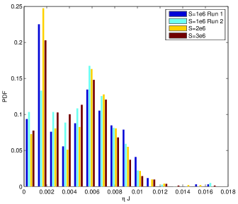
Let us now take a more detailed look into the statistics of current sheets. Figure 8 shows the probability distribution functions (PDFs) of for , from cases with . The case has been done with two runs. The PDFs of from different runs clearly show a degree of similarity, which lends some support to our hypothesis of similarity across systems of different global Lundquist number. However, we also notice some differences between the PDFs from different runs. Even the two runs with show a significant variation in the PDFs. Therefore, more study is needed to further assess the validity of our hypothesis. Ideally the same global setting should be repeated many times with different random seeds for better statistics, but that is computationally too expensive to be done at the present time.
Before we conclude this Section, we remark on a few subtle issues. In the heuristic argument given above, we have used the quantity to estimate the reconnection rate. Strictly speaking, this is valid when the X-point and the stagnation point of the flow coincide, which is not necessarily the case when the reconnection layer is embedded with multiple X-points and plasmoids. Notwithstanding this caveat, we generally find that the peak value of is a reasonable measure of the reconnection rate.
We also address the issue of whether random forcing, by itself, can significantly enhance the reconnection rate. An estimate of the effect of reconnection rate due to random fluctuations is the quantity at the reconnection layer, where is the random velocity fluctuation. Our estimates indicate that the contribution of random fluctuations is less than 1% of the observed reconnection rate in the high- regime. This conclusion is reinforced by the fact that in the plasmoid stable regime, the variations in for different are negligible. This is qualitatively different from a recent turbulent magnetic reconnection study by Loureiro et al.,Loureiro et al. (2009) where the system is more strongly driven, and the reconnection rate shows a noticeable dependence on the magnitude of the forcing even for a Lundquist number as low as .
IV Summary and Conclusion
In summary, we have shown through a series of simulations that resistive MHD can achieve a fast reconnection rate in the high-Lundquist-number regime. Fast reconnection is facilitated by the plasmoid instability. The resultant reconnection rate is independent of and is weakly dependent on the noise level. We have verified the scaling of the number of plasmoids in the linear regime, as predicted in Refs. Loureiro et al. (2007); Bhattacharjee et al. (2009). In the nonlinear regime, the number of plasmoids follows a steeper scaling and is proportional to . We also have done statistical studies of the local current sheets, and found that the current sheet thickness and length both scale as , while the current density scales as . These findings are consistent with our heuristic argument and the claim that the reconnection rate is independent of in the high- regime.
The fast reconnection rate we have obtained is approximately , which is similar to the values from other recent resistive MHD studies,Bhattacharjee et al. (2009); Cassak et al. (2009) but is smaller than the typical reconnection rate from collisionless two-fluid or particle-in-cell simulations by an order of magnitude. Which rate will be realized depends on how collisional the system is. If the Sweet-Parker thickness is greater than the ion skin depth (or the ion Larmor radius at the sound speed, , if there is a guide field) in a system, a Sweet-Parker layer is likely to form first. On the other hand, if (or ), the reconnection would likely proceed dominated by collisionless effects.Aydemir (1992); Ma and Bhattacharjee (1996); Dorelli and Birn (2003); Bhattacharjee (2004); Cassak et al. (2005, 2007) An interesting regime that has not drawn much attention before is when (or ) but . Then we expect the plasmoid instability to set in and the primary Sweet-Parker layer will break into segments. This brings the thickness further down to . If (or ) then the system is still dominated by collisional effects and we may end up getting a reconnection rate of . However, if (or ) then the system will be in the collisionless regime. It is possible the reconnection rate will be further enhanced. Indeed, the recent particle-in-cell simulation by Daughton et al. suggests this possibility Daughton et al. (2009) but more needs to be done to determine if this is a general trend.
Acknowledgements.
The authors would like to thank Dr. Brian P. Sullivan, Prof. Kai Germaschewski, Dr. William Fox, Dr. Hongang Yang, Prof. Barrett N. Rogers, and Prof. Chung-Sang Ng for beneficial conversations. We also acknowledge an anonymous referee for many constructive suggestions. This work is supported by the Department of Energy, Grant No. DE-FG02-07ER46372, under the auspice of the Center for Integrated Computation and Analysis of Reconnection and Turbulence (CICART) and the National Science Foundation, Grant No. PHY-0215581 (PFC: Center for Magnetic Self-Organization in Laboratory and Astrophysical Plasmas). Computations were performed on facilities at National Energy Research Scientific Computing Center and the Zaphod Beowulf cluster, which was funded in part by the Major Research Instrumentation program of the National Science Foundation, Grant No. ATM-0424905.References
- Bhattacharjee et al. (2009) A. Bhattacharjee, Y.-M. Huang, H. Yang, and B. Rogers, Phys. Plasmas 16, 112102 (2009).
- Daughton et al. (2009) W. Daughton, V. Roytershteyn, B. J. Albright, H. Karimabadi, L. Yin, and K. J. Bowers, Phys. Rev. Lett. 103, 065004 (2009).
- Sweet (1958) P. A. Sweet, Nuovo Cimento Suppl. Ser. X 8, 188 (1958).
- Parker (1963) E. N. Parker, Astrophys. J. Suppl. 8, 177 (1963).
- Petschek (1964) H. E. Petschek, in AAS/NASA Symposium on the Physics of Solar Flares, edited by W. N. Hess (NASA, Washington, DC, 1964), p. 425.
- Biskamp (2000) D. Biskamp, Magnetic Reconnection in Plasmas (Cambridge University Press, 2000).
- Bulanov et al. (1979) S. V. Bulanov, J. Sakai, and S. I. Syrovatskii, Sov. J. Plasma Phys. 5, 157 (1979).
- Lee and Fu (1986) L. C. Lee and Z. F. Fu, J. Geophys. Res. 91, 6807 (1986).
- Biskamp (1986) D. Biskamp, Phys. Fluids 29, 1520 (1986).
- Yan et al. (1992) M. Yan, H. C. Lee, and E. R. Priest, Journal of Geophysical Research 97, 8277 (1992).
- Shibata and Tanuma (2001) K. Shibata and S. Tanuma, Earth Planets Space 53, 473 (2001).
- Lapenta (2008) G. Lapenta, Phys. Rev. Lett. 100, 235001 (2008).
- Loureiro et al. (2007) N. F. Loureiro, A. A. Schekochihin, and S. C. Cowley, Phys. Plasmas 14, 100703 (2007).
- Longcope and Strauss (1993) D. W. Longcope and H. R. Strauss, Phys. Fluids B 5, 2858 (1993).
- Uzdensky and Kulsrud (2000) D. A. Uzdensky and R. M. Kulsrud, Phys. Plasmas 7, 4018 (2000).
- Alvelius (1999) K. Alvelius, Phys. Fluids 11, 1880 (1999).
- Guzdar et al. (1993) P. N. Guzdar, J. F. Drake, D. McCarthy, A. B. Hassam, and C. S. Liu, Phys. Fluids B 5, 3712 (1993).
- Samtaney et al. (2009) R. Samtaney, N. F. Loureiro, D. A. Uzdensky, A. A. Schekochihin, and S. C. Cowley, PRL 103, 105004 (2009).
- Loureiro et al. (2009) N. F. Loureiro, D. A. Uzdensky, A. A. Schekochihin, S. C. Cowley, and T. A. Yousef, Mon. Not. R. Astron. Soc. 399, L146 (2009).
- Cassak et al. (2009) P. A. Cassak, M. A. Shay, and J. F. Drake, Phys. Plasmas 16, 120702 (2009).
- Aydemir (1992) A. Y. Aydemir, Phys Fluids B-Plasma Phys. 4, 3469 (1992).
- Ma and Bhattacharjee (1996) Z. W. Ma and A. Bhattacharjee, Geophys. Res. Lett. 23, 1673 (1996).
- Dorelli and Birn (2003) J. C. Dorelli and J. Birn, J. Geophys. Res. 108, 1133 (2003).
- Bhattacharjee (2004) A. Bhattacharjee, Annu. Rev. Astron. Astrophys. 42, 365 (2004).
- Cassak et al. (2005) P. A. Cassak, M. A. Shay, and J. F. Drake, Phys. Rev. Lett. 95, 235002 (2005).
- Cassak et al. (2007) P. A. Cassak, J. F. Drake, and M. A. Shay, Phys. Plasmas 14, 054502 (2007).