Basis set effects on the hyperpolarizability of CHCl₃: Gaussian-type orbitals, numerical basis sets and real-space grids

Abstract

Calculations of the hyperpolarizability are typically much more difficult to converge with basis set size than the linear polarizability. In order to understand these convergence issues and hence obtain accurate ab initio values, we compare calculations of the static hyperpolarizability of the gas-phase chloroform molecule (CHCl₃) using three different kinds of basis sets: Gaussian-type orbitals, numerical basis sets, and real-space grids. Although all of these methods can yield similar results, surprisingly large, diffuse basis sets are needed to achieve convergence to comparable values. These results are interpreted in terms of local polarizability and hyperpolarizability densities. We find that the hyperpolarizability is very sensitive to the molecular structure, and we also assess the significance of vibrational contributions and frequency dispersion.

I Introduction

Chloroform (CHCl₃) is a widely used solvent in measurements of nonlinear optical properties of organic chromophores, using techniques such as electric-field-induced second-harmonic generation (EFISH) and hyper-Rayleigh scattering (HRS).Kaatz et al. (1998); Das (2006) It is sometimes also used as an internal reference.Clays and Persoons (1991) However, assumptions have to made to extract molecular hyperpolarizabilities from these measurements, in particular from EFISH which actually measures a third-order response function. For calibration purposes, either absolute measurements or ab initio calculations are needed to convert between the different combinations of tensor components of the hyperpolarizability measured in the EFISH and HRS experiments. However, very early calculations, which have been recognized as unsatisfactory by their authors,Karna and Dupuis (1990) have heretofore been used for such conversions.Kaatz et al. (1998) Consequently there is a need for better understanding of the convergence issues and for more accurate ab initio calculations. Toward this end we have carried out a systematic study of the second-order hyperpolarizability $\beta$ of chloroform using several theoretical methods. In an effort to obtain high-quality results which improve on earlier calculations, we have based our calculations on an accurate experimental structure and also considered both frequency-dependence and vibrational contributions, effects which are typically neglected in other calculations.

Although our presentation is restricted to a single system, the methodology is more general and hence many of our results will likely be applicable to many other cases. Likewise, the quantitative comparison of several theoretical methods is both novel and of general interest. Finally we believe our interpretation of the linear and nonlinear response in terms of local polarizability densities provides a useful way of understanding the local contributions to the polarizability from various parts of a molecule.

Chloroform is of particular theoretical interest because its hyperpolarizability is challenging to measure experimentally due its small magnitude compared to typical experimental errors, and hence the available measurements have both positive and negative values, with large error bars.Kaatz et al. (1998); Miller and Ward (1977) Similarly, this nonlinear property has proved to be quite difficult to calculate theoretically, as the results exhibit a large dependence on the quality of the basis set used, both for DFT and coupled-cluster methods,Davidson et al. (2006); Hammond and Kowalski (2009) as well as the molecular geometry. One of the main purposes of this paper is to investigate the reasons for these difficulties using three different basis set approaches: i) Gaussian-type orbitals (GTOs); ii) numerical basis sets; and iii) real-space grids, all with comparable treatments of exchange and correlation. The importance of different aspects of the basis sets (diffuseness, polarization, etc.) was studied systematically by changing the number of GTOs, the cutoff radii of the numerical basis sets, and the extent and density of the real-space grids. In order to interpret these results, we also studied the spatial distribution of the dielectric properties using the concepts of polarizability- and hyperpolarizability-densities, as well as first- and second-order electric-field-perturbed densities.Chopra et al. (1989); Nakano et al. (2005) In addition, we also investigated the dependence of polarization properties on the choice of exchange-correlation (XC) functionals and the correlation level by means of DFT, HF, MP2 and CCSD methods. We also briefly discuss the dependence of the results on the molecular geometry, which was found to have a significant influence on the calculated hyperpolarizability.

Unless noted explicitly, the experimental molecular geometry of Colmont et al.Colmont et al. (1998) was used throughout this work: $r_{\mathrm{CH}}=1.080$ Å, $r_{\mathrm{CCl}}=1.760$ Å and $\angle{\mathrm{HCCl}}=108.23$^∘. The molecule was located with its center of mass at the origin, and oriented with the CH bond along the positive $z$-direction and one HCCl angle in the $yz$-plane. Since chloroform has C_3v point-group symmetry, the following symmetry relations hold for the linear polarizability $\alpha$ and hyperpolarizability $\beta$: $\alpha_{xx}=\alpha_{yy}$, $\beta_{xxy}=-\beta_{yyy}$ and $\beta_{xxz}=\beta_{yyz}$. In the static case Kleinman symmetryKleinman (1962) also applies. Thus the $\alpha_{yy}$, $\alpha_{zz}$, $\beta_{yyy}$, $\beta_{yyz}$ and $\beta_{zzz}$ components fully describe the polarizability and hyperpolarizability tensors; all other permutations of the indices are equivalent. In the dynamic case at non-zero frequency, however, the components of $\beta_{ijk}\left(-2\omega;\omega,\omega\right)$ are not all equivalent: $\beta_{yyz}=\beta_{yzy}\neq\beta_{zyy}$. Here we use the Taylor convention for hyperpolarizabilities.Willetts et al. (1992)

From our calculated tensor components we can calculate the isotropically averaged polarizability $\bar{\alpha}=\frac{1}{3}\sum_{i}\alpha_{ii}$, the second-order hyperpolarizability coefficient, and the EFISH hyperpolarizability in the direction of the dipole moment $\beta_{\parallel i}=\frac{1}{5}\sum_{j}\left(\beta_{ijj}+\beta_{jij}+\beta_{jji}\right)$. In the C_3v point group, these relations reduce to $\bar{\alpha}=\frac{1}{3}(2\alpha_{yy}+\alpha_{zz})$, $\beta_{\parallel z}=\frac{3}{5}(2\beta_{yyz}+\beta_{zzz})$. We also calculate the hyperpolarizability for hyper-Rayleigh scattering in the VV polarization, as given by Cyvin et al.Cyvin et al. (1965) for the static case (where Kleinman symmetry holds) and the generalization of Bersohn et al.Bersohn et al. (1966) for the dynamic case. In the static case for C_3v symmetry

$$\left[\beta_{\mathrm{HRS}}^{\mathrm{VV}}\right]^{2}=\frac{8}{35}\beta_{yyy}^{2}+\frac{1}{7}\beta_{zzz}^{2}+\frac{24}{35}\beta_{yyz}^{2}+\frac{12}{35}\beta_{yyz}\beta_{zzz}.$$ (1)

This quantity has only been measured for liquid chloroform;Kaatz et al. (1998) measurements are not available for the gas phase.

Our best results for each method generally exhibit a consistent agreement among themselves and lend confidence to the overall quality of our calculations compared to earlier work. Achieving this consistency points to the need for a comprehensive and well balanced description of all regions of the system: namely, the outlying regions of the molecule, the short C-H bond, and the Cl atoms. A key finding is that the local contributions to the $\beta_{zzz}$ response of the Cl atoms and the C-H bond are of opposite sign and tend to cancel, thus explaining the relatively slow convergence of this component with respect to the basis set size. This behavior, together with the near cancellation of the $\beta_{yyz}$ and $\beta_{zzz}$ components, leads to the relatively small value of $\beta_{\parallel}$ of chloroform. By contrast, the HRS hyperpolarizability converges much more quickly since it is an incoherent process which is mostly given by a sum of squares of tensor components that do not cancel.

II Methods

II.1 Gaussian-Type Orbitals

The GTO polarization properties were calculated using finite-field perturbation theory (FFPT). The electric-field strengths $\mathcal{E}$ used were 0.00, $\pm$0.01 and $\pm$0.02 au. The different components of the induced dipole moment were fit to a 4th-order polynomial to obtain the polarizability and hyperpolarizability tensors. Using analytic derivatives available at the Hartree-Fock level, we find that the properties obtained with the FFPT method agree to 0.1% or better. The effects of the basis set size and diffuse quality were studied using Dunning’s double- through quintuple-$\zeta$ correlation-consistent sets,Dunning (1989); Woon and Dunning (1993) with and without augmentation exponents, and with additional diffuse exponents. We also used Sadlej’s HyPol basis set,Pluta and Sadlej (1998) which is specifically designed for the calculation of nonlinear response properties. In this paper, for simplicity, these basis sets will be referred to as aVDZ and VDZ (for aug-cc-pVDZ and cc-pVDZ, respectively), aVTZ and VTZ (for aug-cc-pVTZ and cc-pVTZ), etc. The HyPol set will be abbreviated as HP. The basis set labeled aV5Zs corresponds to the aV5Z set, where the $g$ and $h$ functions were removed from the C and Cl atoms and the $f$ and $g$ were removed from the H atom. The d-aV5Zs basis set corresponds to the aV5Zs set augmented with (0.014184, 0.009792, 0.025236) and (0.017244, 0.012528, 0.036108) ($s$,$p$,$d$) exponents on the C and Cl atoms, respectively and (0.004968, 0.026784) ($s$,$p$) exponents on the H atom.

Throughout this paper, unless otherwise specified, we use Hartree atomic units $e=\hbar=m=1$ with distances in Bohr ($a_{0}\approx$ 0.529 Å) and energies in Hartrees $\approx$ 27.2 eV. The effect of electron correlation on these all-electron calculations was studied with the LDA,Perdew and Zunger (1981) PBE,Perdew et al. (1996) B3LYP,Becke (1993); Stephens et al. (1994) and BMKBoese and Martin (2004) exchange-correlation density functionals, as well as with the HF, MP2 and CCSD methods. Other XC functionals, such as the CAM-B3LYP functional,Yanai et al. (2004) have been used for hyperpolarizability calculations, but we have not included them since they have not shown a systematic improvement with respect to CCSD.Hammond and Kowalski (2009) All GTO calculations were performed with Gaussian 03.Frisch et al. (2003)

II.2 Real-Space Grids

For the real-space grid calculations we used ab initio density-functional theory with a real-space basis, as implemented in Octopus.Castro et al. (2006); Marques et al. (2003) The polarizability and hyperpolarizability were calculated by linear response via the Sternheimer equation and the $2n+1$ theorem.Andrade et al. (2007) This approach, also known as density-functional perturbation theory, avoids the need for sums over unoccupied states. The PBE exchange-correlation functional was used for the ground state, and the adiabatic LDA kernel was used for the linear response. All calculations used Troullier-Martins norm-conserving pseudopotentials.Troullier and Martins (1991)

The molecule was studied as a finite system, with zero boundary conditions for the wavefunction on a large sphere surrounding the molecule, as described below. Convergence was tested with respect to the real-space grid spacing and the radius of the spherical domain. The grid spacing required is determined largely by the pseudopotential, as it governs the fineness with which spatial variations of the wavefunctions can be described as well as the accuracy of the finite-difference evaluation of the kinetic-energy operator. The spacing $\lambda$ can be converted to an equivalent plane-wave cutoff via $E_{c}=({\hbar^{2}}/{2m})({2\pi}/{\lambda})^{2}$, where $E_{c}$ is the cutoff energy for both the charge density and wavefunctions. The sphere radius determines the maximum spatial extent of the wavefunctions.

With tight numerical tolerances in solving the Kohn-Sham and Sternheimer equations, we can achieve a precision of 0.01 au or better in the converged values of the tensor components of $\beta$. We also did two additional kinds of calculations. For comparison to the nonlinear experiments, which used incoming photons of wavelength 1064 nm (energy 1.165 eV), we also performed dynamical calculations at this frequency via time-dependent density-functional theory (TDDFT). To compare directly to the results from finite-field perturbation theory with the other basis sets, we also calculated the dielectric properties via finite differences using electric-field strengths of $\pm$0.01 and $\pm$0.015 au.

II.3 Numerical Basis Sets

The numerical basis set (NBS) calculations were performed with the SiestaE. Artacho, D. Sánchez-Portal, P. Ordejón, A. García, and J. M. Soler (1999); J. M Soler, E. Artacho, J. D. Gale, A. García, J. Junquera, P. Ordejón, and D. Sánchez-Portal (2002) code and used Troullier-Martins norm-conserving pseudopotentials.Troullier and Martins (1991) As in the GTO calculations described in section II.1, the polarization properties were obtained using FFPT with electric-field strengths of 0.00, $\pm$0.01 and $\pm$0.02 au. The NBSs use a generic linear combination of numerical atomic orbitals (NAOs) that are forced to be zero beyond a cutoff radius $r_{c}$.Sankey and Niklewski (1989) Rather than using a fixed $r_{c}$ for all atoms, a common confinement-energy shift is usually enforced, resulting in well-balanced basis sets.J. M Soler, E. Artacho, J. D. Gale, A. García, J. Junquera, P. Ordejón, and D. Sánchez-Portal (2002) In general, multiple radial functions with the same angular dependence are introduced to enhance the flexibility of the basis set. This results in a so-called multiple-$\zeta$ scheme similar to the standard split-valence approach used for GTOs.Huzinaga (1985); Szabo and Ostlund (1982) Polarization functions can also be added using the approach described in Ref. J. M Soler, E. Artacho, J. D. Gale, A. García, J. Junquera, P. Ordejón, and D. Sánchez-Portal, 2002. Typically, double-$\zeta$ sets with a single polarization function (DZP) are sufficient in linear-response calculations. However, we found that a DZP set is insufficient for nonlinear properties. Instead of performing an optimization of the NBSs, we improved their flexibility by adding $\zeta$-functions, and controlling their splitting.J. M Soler, E. Artacho, J. D. Gale, A. García, J. Junquera, P. Ordejón, and D. Sánchez-Portal (2002) By varying the “norm-splitting” parameter in Siesta, we can control the flexibility in different regions of the radial functions, resulting in the cutoff radii and energy shifts shown in Tables 1 and 2.

Table 1: Parameters used in the definition of the numerical basis sets: energy shifts $\delta\epsilon$ and cutoff radii $r_{c}^{l}(\mathrm{X})$ of the first-$\zeta$ for angular momentum $l$ and atom X. All values are in atomic units.

Parameter	DZP	QZTPe4	5Z4Pe5	5Z4Pe6	5Z4Pe7	5Z4Pe8
$\delta\epsilon$	$10^{-2}$	$10^{-4}$	$10^{-5}$	$10^{-6}$	$10^{-7}$	$10^{-8}$
$r_{c}^{s}(\mathrm{C})$	$4.088$	$6.574$	$7.832$	$8.875$	$10.056$	$11.114$
$r_{c}^{p}(\mathrm{C})$	$4.870$	$8.655$	$10.572$	$12.283$	$14.271$	$15.772$
$r_{c}^{s}(\mathrm{H})$	$4.709$	$8.164$	$9.972$	$11.586$	$13.461$	$14.877$
$r_{c}^{s}(\mathrm{Cl})$	$3.826$	$5.852$	$6.799$	$7.704$	$8.730$	$9.410$
$r_{c}^{p}(\mathrm{Cl})$	$4.673$	$7.514$	$8.951$	$10.400$	$11.784$	$13.024$

Table 2: Parameters used in the definition of the numerical basis sets: splitting radii $r_{c}^{l}(\mathrm{X})$ associated with a given norm splitting for angular momentum $l$ and atom X. All values are in atomic units.

Norm splitting	0.0015	0.0150	0.1500	0.6000
$r_{c}^{s}(\mathrm{C})$	$6.574$	$5.120$	$3.519$	$2.272$
$r_{c}^{p}(\mathrm{C})$	$8.548$	$6.332$	$3.841$	$2.005$
$r_{c}^{s}(\mathrm{H})$	$8.690$	$6.600$	$4.155$	$2.223$
$r_{c}^{s}(\mathrm{Cl})$	$5.707$	$4.557$	$3.252$	$2.292$
$r_{c}^{p}(\mathrm{Cl})$	$7.328$	$5.566$	$3.639$	$2.235$

Finally, the NBS calculations used a common (20.0 Å)³ cell and real-space grid with a plane-wave-equivalent cutoff of 250 Ry for the calculation of the Hartree and exchange-correlation potentials. This corresponds to a real-space mesh spacing of about 0.1 Å.

II.4 Linear and Nonlinear Response Densities

The origin of the slow convergence of the hyperpolarizability with respect to the quality of the basis set is difficult to understand by studying only the total quantities. A more informative analysis can be obtained from the spatial distribution of the dielectric properties. Thus, we have calculated the linear and nonlinear response densities, as well as their associated properties. Here we will focus on the response densities induced by an electric field in the $z$-direction. The first-order density is defined as

$$\rho_{z}^{(1)}\left(r\right)=\frac{\partial\rho}{\partial\mathcal{E}_{z}},$$ (2)

and the linear polarizability $\alpha_{zz}\left(r\right)$ as

$$\alpha_{zz}\left(r\right)=\rho_{z}^{(1)}\left(r\right)z.$$ (3)

The second-order response density and associated hyperpolarizability are defined similarly:

$$\rho_{zz}^{(2)}\left(r\right)=\frac{\partial^{2}\rho}{\partial\mathcal{E}_{z}^{2}},$$ (4)

$$\beta_{zzz}\left(r\right)=\rho_{zz}^{(2)}\left(r\right)z.$$ (5)

These response densities are all calculated using finite differences. For the real-space grids, our Sternheimer approach provides only the linear response density and polarizability density, but not the nonlinear response and hyperpolarizability densities.

Unlike the total properties, the spatial distributions of polarizabilities and hyperpolarizabilities as defined above depend on the origin of coordinates. Throughout this work we chose a center-of-mass reference for the spatial distributions. To understand the role that different regions of the molecule play in the total properties, we have devised a partitioning scheme for the spatial distribution corresponding to the spaces occupied roughly by the Cl atoms and C-H bond. That is, we divide space into two regions by constructing three planes, each orthogonal to one of the C-Cl bonds, and passing through a point located 40% along the C-Cl bond from the C atom, which corresponds approximately to the density minimum along the C-Cl bond. The first region (“CH”) consists of all the space above the three planes, and contains the C-H bond, while the second (“Cl”) covers the remainder of the space, including the three Cl atoms. We have integrated the various densities in each region numerically to find its contribution to the total.

III Results and Discussion

III.1 Structure

Although all the results presented in later sections were obtained for the experimental geometry determined by Colmont et al.,Colmont et al. (1998) here we briefly discuss the effect of the structural parameters on the dielectric properties. We compared properties obtained for experimental structuresColmont et al. (1998); Jen and Lide (1962) with theoretical structures optimized using the PBE functional, one obtained with the aVQZ basis in Gaussian03,Davidson et al. (2006) and the other with a real-space grid in Octopus. The parameters for each structure are listed in Table 3. The linear and nonlinear properties for each structure were calculated with the Sternheimer method in Octopus, using a radius of 17 $a_{0}$ and a spacing of 0.25 $a_{0}$ and the results are summarized in Table 4. Our calculations show that the dipole moment and polarizability are not affected much, but the hyperpolarizability varies significantly with structure. Individual tensor components of the hyperpolarizability do not change by more than $\sim$30%, but since $\beta_{\parallel}$ is a sum of large positive and negative components, it can change sign, and change by orders of magnitude depending on the structure. Note, however, that all geometries give results consistent with the large relative error bar on the gas-phase experimental value of $\beta_{\parallel}=1\pm 4$ au.Kaatz et al. (1998)

Table 3: Structural parameters used in the study of the variation of the dielectric properties of CHCl₃ with structure. PBE/aVQZ and PBE/RS refer to PBE-optimized structures using the aVQZ GTO in Gaussian and a real-space grid in Octopus, respectively. Bond lengths are in Å and angles in degrees. The experimental structure from Ref. Colmont et al., 1998 was used for all our subsequent calculations.

Source	$r$(C-H)	$r$(C-Cl)	∠HCCl
Expt.Jen and Lide (1962)	1.100 $\pm$ 0.004	1.758 $\pm$ 0.001	107.6 $\pm$ 0.2
Expt.Colmont et al. (1998)	1.080 $\pm$ 0.002	1.760 $\pm$ 0.002	108.23 $\pm$ 0.02
PBE/aVQZDavidson et al. (2006)	1.090	1.779	107.7
PBE/RS	1.084	1.769	107.6

Table 4: Dielectric properties of various structures for CHCl₃ described in Table 3, as calculated by DFT on a real-space grid with radius 17 $a_{0}$ and spacing 0.25 $a_{0}$, compared with the experimental values of the dipole moment and the electronic contribution to the polarizability. PBE/aVQZ and PBE/RS refer to the structures described in Table 3. All values are in atomic units (au).

Structure	$\mu_{z}$	$\alpha_{yy}$	$\alpha_{zz}$	$\beta_{yyy}$	$\beta_{yyz}$	$\beta_{zzz}$	$\bar{\alpha}$	$\beta_{\parallel}$	$\beta_{\mathrm{HRS}}^{\mathrm{VV}}$
Expt.Jen and Lide (1962)	$0.395$	$66.14$	$47.22$	$27.09$	$-14.41$	$28.47$	$59.83$	$-0.21$	$16.89$
Expt.Colmont et al. (1998)	$0.399$	$66.02$	$47.00$	$27.12$	$-16.36$	$26.92$	$59.68$	$-3.49$	$17.44$
PBE/aVQZDavidson et al. (2006)	$0.401$	$67.17$	$47.35$	$27.23$	$-14.11$	$27.76$	$60.57$	$-0.27$	$16.79$
PBE/RS	$0.397$	$66.66$	$47.12$	$27.29$	$-14.26$	$28.92$	$60.15$	$0.24$	$16.96$
Expt.	0.409$\pm$0.008  Reinhart et al. (1970)	61$\pm$5  Stuart and Volkmann (1933)	45$\pm$3  Stuart and Volkmann (1933)				56$\pm$4  Stuart and Volkmann (1933)	1$\pm$4  Kaatz et al. (1998)

III.2 Gaussian-Type Orbitals

Table 5 shows the effect of the basis set size on the dielectric properties calculated with the PBE functional and GTOs. The results from this work agree well with those reported by Davidson et al.Davidson et al. (2006) In the case of the dipole moment, we also find agreement to within 1% of the experimental value of 0.409 $\pm$ 0.008 auReinhart et al. (1970) for every basis set except VDZ. (The quality of the basis set roughly increases down the table.) The polarizabilities agree well with the experimentally measured values at 546 nm (2.27 eV);Stuart and Volkmann (1933) these quantities are optical polarizabilities which contain only an electronic contribution and have minimal dispersion. Indeed, our real-space TDDFT calculations (Section III.3) at 532 nm (2.24 eV) give $\alpha_{yy}$ = 68.827 au and $\alpha_{zz}$ = 48.405 au, a small increase from the static and 1064 nm results, and basically consistent with the experimental values. We can also compare to a measurement of the static isotropically averaged polarizability of 64 $\pm$ 3 au.Miller et al. (1981) To compare with our result for the average electronic polarizability, we subtract the estimated vibrational contribution of 4.5 au calculated from experimental data (no error bar provided),Bishop and Cheung (1982) yielding 60 au, which agrees with the predicted values within 0.4%. To verify this comparison, we have also computed the vibrational component of the polarizability from first principles, obtaining a value of 6.3 au, in reasonable agreement with the above estimate. This value was obtained by first doing a standard Gaussian 03Frisch et al. (2003) calculation of vibrational-frequencies at the PBE/aug-cc-pVTZ level, using a molecular structure optimized at the same level. The polarizability is then calculated as described in Ref. Kirtman et al., 1996.

Table 5: Effect of the GTO basis set quality on the components of the dielectric properties of CHCl₃ calculated with the PBE functional. All values are in atomic units.

Basis Set	$\mu_{z}$	$\alpha_{yy}$	$\alpha_{zz}$	$\beta_{yyy}$	$\beta_{yyz}$	$\beta_{zzz}$	$\bar{\alpha}$	$\beta_{\parallel}$	$\beta_{\mathrm{HRS}}^{\mathrm{VV}}$
VDZ	$0.426$	$46.36$	$25.82$	$19.64$	$-8.43$	$-44.25$	$39.51$	$-36.66$	$23.33$
VTZ	$0.417$	$54.57$	$34.08$	$0.52$	$-3.35$	$-37.20$	$47.74$	$-26.33$	$15.75$
VQZ	$0.407$	$59.92$	$39.76$	$-5.83$	$-2.88$	$-25.57$	$53.20$	$-18.80$	$10.90$
V5Z	$0.405$	$61.65$	$41.93$	$-6.12$	$-5.70$	$-25.85$	$55.08$	$-22.35$	$12.64$
aVDZ	$0.412$	$63.29$	$44.35$	$8.53$	$-11.35$	$2.62$	$56.98$	$-12.05$	$9.78$
aVTZ	$0.408$	$64.91$	$46.03$	$14.67$	$-11.81$	$11.72$	$58.62$	$-7.14$	$10.82$
aVQZ	$0.406$	$65.50$	$46.61$	$21.15$	$-13.81$	$19.52$	$59.21$	$-4.86$	$13.96$
aV5Z	$0.404$	$65.69$	$46.71$	$22.02$	$-14.26$	$18.65$	$59.36$	$-5.92$	$14.45$
aV5Zs	$0.404$	$65.67$	$46.70$	$21.78$	$-14.01$	$17.92$	$59.34$	$-6.07$	$14.24$
d-aV5Zs	$0.404$	$65.70$	$46.79$	$27.35$	$-15.31$	$22.27$	$59.40$	$-5.01$	$16.90$
HP	$0.405$	$65.51$	$46.60$	$27.64$	$-15.54$	$22.93$	$59.21$	$-4.89$	$17.12$
Expt.	0.409$\pm$0.008  Reinhart et al. (1970)	61$\pm$5  Stuart and Volkmann (1933)	45$\pm$3  Stuart and Volkmann (1933)				56$\pm$4  Stuart and Volkmann (1933)	1$\pm$4  Kaatz et al. (1998)

For the hyperpolarizability, Davidson et al. also obtain good agreement between theory and experiment provided the values of $\beta_{\parallel}$ calculated with the aVDZ, aVTZ and aVQZ correlation-consistent basis sets are smoothly extrapolated to the complete basis set limit.Peterson et al. (1993) If the same extrapolation scheme is applied to our results for $\beta_{\parallel}$ given in Table 5, however, we obtain a value of -2.89 au, which is barely within the error of the experimental value of 1 $\pm$ 4 au. This extrapolated value also differs from the value of 0.35 au obtained by Davidson et al. The difference can be attributed to the different geometries used: In this work we used the experimentally determined structure, while Davidson et al. used the theoretical structures obtained with the aVDZ, aVTZ and aVQZ basis sets. When we use the aVTZ-optimized geometry in our calculations instead of the experimental one, we obtain an extrapolated value of 0.6 au, which is consistent with the Davidson et al. value. Our calculations also included the aV5Z basis set, the next basis set in the correlation-consistent series. When this set is included in the extrapolation, our predicted value is lowered to -5.29 au. The sudden reduction of the estimated complete basis set value upon inclusion of the aV5Z set indicates that the convergence of $\beta_{\parallel}$ is not smoothly monotonic. Therefore the basis set sequence aVDZ-aV5Z is not well adapted to the extrapolation of this property. This stems from the fact that although the individual components $\beta$ rise in a reasonably monotonic way, small deviations in their progression and their near cancellation lead to sudden changes in $\beta_{\parallel}$.

Table 6: Effect of the exchange-correlation (XC) treatment on the components of the dielectric properties of CHCl₃ calculated with the HP GTO basis set. All values are in atomic units.

XC	$\mu_{z}$	$\alpha_{yy}$	$\alpha_{zz}$	$\beta_{yyy}$	$\beta_{yyz}$	$\beta_{zzz}$	$\bar{\alpha}$	$\beta_{\parallel}$	$\beta_{\mathrm{HRS}}^{\mathrm{VV}}$
LDA	$0.414$	$65.95$	$47.03$	$28.89$	$-16.21$	$22.56$	$59.64$	$-5.91$	$17.83$
PBE	$0.405$	$65.51$	$46.60$	$27.64$	$-15.54$	$22.93$	$59.21$	$-4.89$	$17.12$
BMK	$0.453$	$62.13$	$44.77$	$22.56$	$-11.58$	$18.63$	$56.35$	$-2.72$	$13.56$
B3LYP	$0.423$	$63.60$	$45.60$	$21.90$	$-12.99$	$18.98$	$57.60$	$-4.21$	$13.87$
HF	$0.476$	$58.98$	$42.76$	$13.57$	$-7.58$	$13.02$	$53.57$	$-1.28$	$8.48$
MP2	$0.424$	$62.13$	$45.18$	$15.03$	$-9.75$	$16.47$	$56.48$	$-1.82$	$10.03$
CCSD	$0.425$	$61.54$	$44.88$	$16.51$	$-10.31$	$16.81$	$55.99$	$-2.29$	$10.78$
Expt.	0.409$\pm$0.008  Reinhart et al. (1970)	61$\pm$5  Stuart and Volkmann (1933)	45$\pm$3  Stuart and Volkmann (1933)				56$\pm$4  Stuart and Volkmann (1933)	1$\pm$4  Kaatz et al. (1998)

To better understand the convergence of the nonlinear properties with respect to the degree of polarization and diffuseness of the basis sets, we also performed calculations using simplified and enhanced versions of the correlation-consistent basis sets. The results for the non-augmented sets (labeled VDZ-V5Z in Table 5) indicate, as is widely known, that the diffuse exponents are important for the polarizability and crucial for the hyperpolarizability. Even the very large V5Z basis set yields $\beta_{\parallel}$ values that are too low. These values are also less well converged than the much smaller aVDZ augmented set. The polarization functions with high angular momentum (i.e. larger than $d$ and $f$ for the hydrogen and heavy atoms, respectively) play a very small role, as seen from the similarity between the results obtained with the aV5Z set, and the aV5Zs set, where such functions were removed. The results in Table 5 show that this simplification has a negligible effect on the dipole moment and linear polarizability. It also has a fairly small effect ($\sim$3%) on the hyperpolarizability.

The hyperpolarizability values can be further improved by enhancing the diffuseness of the basis set beyond that of the standard Dunning correlation-consistent sets. When the aV5Zs set is extended with a single $d$-function with exponent 0.036108 localized on the Cl atoms, the value of $\beta_{zzz}$ was increased by almost 20%. Further extending the basis set with diffuse functions in the C and H atoms, resulting in the d-aV5Zs set, increases $\beta_{zzz}$ slightly. The d-aV5Zs basis set provides the most saturated GTO results obtained in this work. We note that, from the point of view of augmentation, the basis set d-aV5Zs is equivalent to a d-aug-cc-pV5Z set. That is, the diffuse exponents used are the same as those in the Dunning set. The main difference between the two sets is in the high-angular-momentum exponents, which play a very small role as discussed below. We also attempted to perform the calculations with the t-aug-cc-pV5Z set; however, Gaussian 03 calculations have convergence problems due to the extremely diffuse exponents.

We have also investigated the effect of the tight d-functions on Cl by carrying out calculations with the cc-pV(5+d)Z basis set for Cl augmented with diffuse functions and paired with the d-aV5Zs set from our original calculations for the C and H atoms. However, we find that the tight $d$ functions change the individual components by only about 0.3% and $\beta_{\parallel}$ by only about 2%. Finally, we find that the HyPol basis set, which is approximately equivalent in size to the aVTZ set, yields results that are equivalent to the much larger d-aV5Zs set. This basis set was designed with the explicit purpose of efficiently calculating nonlinear properties. Thus it is not surprising that it provides converged results for a smaller size.

The large variations in $\beta_{\parallel}$ are due largely to changes in $\beta_{zzz}$, for which completing the basis set produces a change of sign and an absolute change of nearly two orders of magnitude. This effect translates into a change of $\beta_{\parallel}$ of nearly an order of magnitude! The same behavior is observed as we complete the numerical basis sets (see Table 8) but not in the case of the real-space calculations (see Table 7). Then the two basis set approaches (GTO and NBS) show similar convergence features as we increase the quality of the basis set.

The variation in the results with the quality of the exchange-correlation treatment is shown in Table 6, in order of increasing level of exchange-correlation accuracy. Note first that the linear properties are rather insensitive to the treatment of exchange and correlation. Also the higher-quality ab initio correlation treatments (MP2 and CCSD) are more or less consistent, while the DFT functionals LDA, PBE, BMK, and B3LYP vary considerably for the nonlinear properties. In the case of the higher-level methods, the properties follow the usual pattern of decreasing the dipole moment and enhancing the polarizability when the treatment of correlation is improved. Compared to the CCSD values, the components of the hyperpolarizability vary by as much as 75%. Judging by the values of $\beta_{\parallel}$, the predicted value increases with improvements in the treatment of correlation. Also the variation among the values can be regarded as an estimate of the error in the results due to approximations in the treatment of exchange and correlation.

III.3 Real-Space Grids

Convergence of the dipole moment, polarizability, and hyperpolarizability is illustrated in Table 7. The total energy was well converged for a spacing of 0.35 $a_{0}$ (equivalent plane-wave cutoff = 20 Ry) and a sphere radius of 12 $a_{0}$. The dipole moment was also well converged with that basis. However, to converge $\beta_{\parallel}$ to better than 0.01 au, a spacing of 0.25 $a_{0}$ (equivalent plane-wave cutoff = 40 Ry) and a sphere radius of 22 $a_{0}$ was required. The convergence of the tensor components of $\beta$ is similar to that of $\beta_{\parallel}$ in absolute terms, i.e. they are also converged to 0.01 au or better with these parameters. Generally, the magnitude of $\beta_{\parallel}$ declines with smaller spacing and larger radius, as the cancellation between the tensor components becomes closer.

Finite-difference calculations were done with the converged grid spacing of 0.25 $a_{0}$, and a sphere radius of 22. $a_{0}$, for comparison to the Sternheimer calculation with the same grid parameters (Table 10). The differences between the linear-response and finite-difference calculations are small, allowing a direct comparison between the results with different basis sets. The use of the LDA kernel in the linear-response results gives a small discrepancy compared to the purely PBE finite-difference results. Fields of 0.015 au rather than 0.02 au as for the other basis sets were used because 0.02 au was out of the linear regime in the real-space calculation. The linear response density $\rho_{z}^{(1)}(r)$ and polarizability density $\alpha_{zz}(r)$ are virtually identical between the finite-difference and linear-response calculations.

Calculations at 1064 nm with the same grid parameters show increases of about 1% in the polarizability, and 10-20% in the hyperpolarizability, as compared to the static case. We find a small violation of Kleinman symmetry here, in that $\beta_{yyz}$ = -18.945 au whereas $\beta_{zyy}$ = -19.448 au.

Table 7: Effect of the real-space-grid quality (radius $R$ and spacing $\lambda$) on the components of the dielectric properties of CHCl₃ calculated with the PBE functional and LDA kernel. All values are in atomic units.

$R$	$\lambda$	$\mu_{z}$	$\alpha_{yy}$	$\alpha_{zz}$	$\beta_{yyy}$	$\beta_{yyz}$	$\beta_{zzz}$	$\bar{\alpha}$	$\beta_{\parallel z}$	$\beta_{\mathrm{HRS}}^{\mathrm{VV}}$
12	$0.25$	$0.398$	$65.921$	$46.924$	$27.975$	$-17.232$	$22.975$	$59.589$	$-6.921$	$17.106$
15	$0.25$	$0.399$	$66.019$	$46.993$	$27.159$	$-16.401$	$26.758$	$59.677$	$-3.629$	$17.461$
17	$0.25$	$0.399$	$66.022$	$46.995$	$27.123$	$-16.363$	$26.921$	$59.680$	$-3.485$	$17.443$
20	$0.25$	$0.399$	$66.023$	$46.995$	$27.119$	$-16.358$	$26.940$	$59.680$	$-3.469$	$17.441$
22	$0.25$	$0.399$	$66.023$	$46.995$	$27.119$	$-16.358$	$26.940$	$59.680$	$-3.468$	$17.441$
17	$0.35$	$0.397$	$66.032$	$47.002$	$27.181$	$-16.233$	$26.921$	$59.689$	$-3.351$	$17.415$
17	$0.30$	$0.399$	$66.029$	$46.989$	$27.168$	$-16.357$	$26.893$	$59.683$	$-3.492$	$17.455$
17	$0.25$	$0.399$	$66.022$	$46.995$	$27.123$	$-16.363$	$26.921$	$59.680$	$-3.485$	$17.443$
17	$0.20$	$0.398$	$66.021$	$46.993$	$27.091$	$-16.355$	$26.903$	$59.678$	$-3.488$	$17.427$
Expt.		0.409$\pm$0.008  Reinhart et al. (1970)	61$\pm$5  Stuart and Volkmann (1933)	45$\pm$3  Stuart and Volkmann (1933)				56$\pm$4  Stuart and Volkmann (1933)	1$\pm$4  Kaatz et al. (1998)

III.4 Numerical Basis Sets

Table 8 shows the variation of the dielectric properties as a function of the quality of the numerical basis set; this is determined by the “energy shift” parameter $\delta\epsilon$ (which is a measure of the spatial extent of the basis) and the number of atomic orbitals.E. Artacho, D. Sánchez-Portal, P. Ordejón, A. García, and J. M. Soler (1999) The default DZP basis set, using the default energy shift of 0.01 au, produces results that are clearly inadequate, being unable to reproduce even the dipole moment. We have found for CHCl₃, that $\delta\epsilon$ must be at least $0.5\times 10^{-6}$ au to obtain a value of $\beta_{\parallel}$ that approaches those obtained with GTOs and real-space grids. Numerical basis set convergence is apparently achieved with $\delta\epsilon=1\times 10^{-8}$ au. The corresponding cutoff radii are 2 to 3 times larger than those produced by the default value of $\delta\epsilon$, clearly matching the need for very diffuse GTOs and large confining spheres for the real-space grids. Moreover, both the valence and polarization parts of the numerical basis set have to be sufficiently flexible to represent the response properties accurately. For instance, at least five valence and four polarization atomic orbitals are needed to obtain accurate results, as is also the case for the GTOs (e.g. the d-aV5Zs set has five $sp$ valence functions plus four $d$- and three $f$-polarization functions). The best value of $\beta_{\parallel}$ is -5.07 au, obtained with the 5Z4Pe8 numerical basis set. This is in good agreement with the value of -5.01 au obtained with the d-aV5Zs GTO set. The close agreement with the GTO results seems to be fortuitous since the components of $\beta$ differ by about 6%.

Table 8: Effect of the numerical basis set quality on the components of the dielectric properties of CHCl₃ calculated with the PBE functional. All values are in atomic units. See Table 1 for a detailed description of each basis set. Note that DZP and DZPe4 are both double-$\zeta$ basis with the same split radius except the first-$\zeta$’s cut-off radius is the same as QZTPe4 for DZPe4.

Basis Set	$\mu_{z}$	$\alpha_{yy}$	$\alpha_{zz}$	$\beta_{yyy}$	$\beta_{yyz}$	$\beta_{zzz}$	$\bar{\alpha}$	$\beta_{\parallel}$	$\beta_{\mathrm{HRS}}^{\mathrm{VV}}$
DZP	$0.240$	$47.30$	$29.99$	$11.68$	$-5.35$	$-29.15$	$41.53$	$-23.91$	$15.02$
DZPe4	$0.361$	$56.45$	$37.62$	$6.05$	$-9.00$	$-39.98$	$50.17$	$-34.79$	$20.39$
QZTPe4	$0.392$	$63.71$	$44.69$	$12.18$	$-10.52$	$-9.90$	$57.37$	$-18.57$	$12.63$
5Z4Pe5	$0.397$	$65.14$	$46.02$	$21.93$	$-13.70$	$14.16$	$58.77$	$-7.96$	$14.17$
5Z4Pe6	$0.398$	$65.41$	$46.23$	$23.71$	$-14.77$	$19.51$	$59.02$	$-6.02$	$15.29$
5Z4Pe7	$0.398$	$65.45$	$46.28$	$24.48$	$-14.93$	$20.18$	$59.06$	$-5.22$	$15.64$
5Z4Pe8	$0.398$	$65.45$	$46.28$	$24.54$	$-14.90$	$21.37$	$59.06$	$-5.07$	$15.68$
Expt.	0.409$\pm$0.008  Reinhart et al. (1970)	61$\pm$5  Stuart and Volkmann (1933)	45$\pm$3  Stuart and Volkmann (1933)				56$\pm$4  Stuart and Volkmann (1933)	1$\pm$4  Kaatz et al. (1998)

III.5 Linear and Nonlinear Response Densities

The origin of the slow convergence of the response properties is difficult to determine just by analyzing their total values for different basis sets. We have found that the differences and similarities between those values can be visualized by computing the real-space distribution of the linear and nonlinear response densities, as well as the associated polarizability and hyperpolarizability densities. For example, Figure 1 shows the linear response density $\rho^{(1)}_{z}\left(r\right)$ calculated with the PBE functional for both the HP GTO basis set and a real-space grid. Clearly, the nearly identical plots confirm that the linear response is equally well represented by both basis sets. Also shown in Figure 1, the polarizability density $\alpha_{zz}\left(r\right)$ reveals the spatial contributions to the total polarizability. For the most part, this property is localized to within $\sim$ 6 au of the center of the molecule, explaining its rapid convergence with respect to the diffuseness of the basis set. Our partitioning scheme for $\alpha_{zz}(r)$ (Table 9) shows that most of the positive contribution to $\alpha_{zz}$ arises from the Cl atoms, in accord with the larger polarizability of the Cl atom. The contribution from the CH bond is significantly smaller and, as can be clearly seen in Figure 1, is the result of counteracting contributions: positive from the H atom and negative from the C-H bond region. Our partitioning also shows that the deficiencies of the GTOs are due mostly to a poorer representation of the Cl atoms.

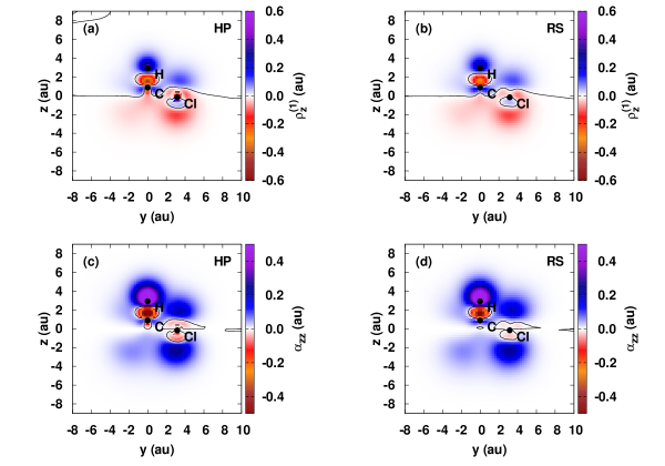
Figure 1: Linear response density $\rho_{z}^{(1)}(r)$ (a-b) and polarizability density $\alpha_{zz}(r)$ (c-d) on one of the HCCl planes of the molecule calculated with a GTO basis set (HP) and a real-space grid (RS) using the PBE functional. The positions of the nuclei are indicated with black dots, and the black lines are isolines. All quantities are in atomic units. Note that the linear response density is quite similar for both methods.

The spatial distributions of the nonlinear response density $\rho_{zz}^{(2)}(r)$ and hyperpolarizability density $\beta_{zzz}(r)$, shown in Figure 2, are also very similar for both the HP GTO set and the real-space grid. The hyperpolarizability density, however, is more delocalized than the polarizability, extending up to $\sim$ 8 au from the center, thus stressing the importance of the diffuse functions in calculations of nonlinear properties. The spatial distribution is also much more complex, with several regions of counteracting contributions. The decomposition shown in Table 9 significantly simplifies the analysis of the densities. It shows that the overall contribution from the C-H bond is negative. This contribution also varies very little with respect to the quality of the basis set. The contribution from the Cl atoms, on the other hand, is positive and varies significantly with the basis set used. For instance, the value obtained for the aVDZ set is almost 30% lower than the aV5Z set. Even the aV5Z basis set does not provide converged results, since the inclusion of extra diffuse exponents (d-aV5Zs set) results in a further increase of 5%. This change is small for the individual Cl contribution, but changes the total $\beta_{zzz}$ component by 16%. Finally, it can again be seen that, although significantly smaller, the HP set provides results that are almost identical to those obtained with the d-aV5Zs one.

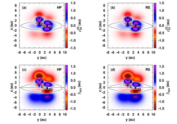
Figure 2: Nonlinear response density $\rho_{zz}^{(2)}(r)$ (a-b) and hyperpolarizability density $\beta_{zzz}(r)$ (c-d) on one of the HCCl planes of the molecule calculated with a GTO basis set (HP) and a real-space grid (RS) using the PBE functional. The positions of the nuclei are indicated with black dots, and the black lines are isolines. All quantities are in atomic units. The nonlinear densities extend much further into space than the linear densities. The agreement between the real-space and GTO methods is nevertheless quite good. The contributions to the hyperpolarizability from the Cl atoms and the CH bond are of opposite sign and, as indicated by the nonlinear response density, have contributions that extend even further into space.

The plots shown in Figure 2 indicate that the CH bond is well saturated with respect to the extent of the diffuse functions. This observation was confirmed by using the d-aV5Zs basis set, which also includes diffuse functions on both the C and H atoms and only slightly improves the results.

Table 9: Partitioning of the linear and nonlinear response properties calculated numerically with GTOs and real-space grids (RS) using the PBE functional together with the numerical sum over the CH and Cl₃ partitions. For comparison the “Analytic” results are given for the integral over all space (without partitioning) from Table V.

Property	Basis Set	CH	Cl3	CH + Cl3	Analytic
$\alpha_{zz}$	aVDZ	$8.91$	$35.42$	$44.33$	$44.35$
	aV5Z	$8.96$	$37.71$	$46.67$	$46.71$
	d-aV5Zs	$8.96$	$37.79$	$46.75$	$46.79$
	HP	$8.92$	$37.67$	$46.59$	$46.60$
	RS	$8.85$	$38.02$	$46.87$	$46.87$
$\beta_{zzz}$	aVDZ	$-43.82$	$46.46$	$2.63$	$2.62$
	aV5Z	$-44.48$	$63.08$	$18.61$	$18.65$
	d-aV5Zs	$-44.31$	$66.54$	$22.24$	$22.27$
	HP	$-44.55$	$67.49$	$22.94$	$22.93$
	RS	$-43.41$	$67.12$	$23.71$	$23.89$

IV Conclusions

We have carried out calculations of the static hyperpolarizability of the gas-phase CHCl₃ molecule, using three different kinds of basis sets: Gaussian-type orbitals, numerical basis sets, and real-space grids. We find that all of these methods can yield quantitatively similar results provided sufficiently large, diffuse basis sets are included in the calculations. In particular diffuse functions are important to obtain accurate results for the polarizability and are crucial for the hyperpolarizability. For GTOs, the standard versions of the augmented Dunning basis set are not adequate to converge the $\beta_{zzz}$ component. However, convergence can be achieved by increasing the diffuse $d$ space on the Cl atoms. Other diffuse functions play smaller role. The overall consistency among the results gives confidence to their reliability and overall accuracy. Based on the size of the basis sets and degree of convergence, the LR real-space values in Table X are likely the most reliable. However, the variation among our results also provides a gauge of their overall theoretical accuracy.

Although the treatment here has been restricted to chloroform, many of the results are more generally applicable. For example, the spatial distributions provided by the linear and nonlinear response densities provides a good visualization tool to understand the basis set requirements for the simulation of linear and nonlinear response. A key finding for chloroform is that the local contributions near the Cl atoms and the CH bond are of opposite sign and tend to cancel, thus explaining the overall weakness of the hyperpolarizability. The molecule’s response is quite extended in space and so real-space grids on a large domain, as well as very extended local orbitals, are required to describe it properly. The frequency-dependence of the polarizability and hyperpolarizability is small, as verified by our time-dependent calculations, and so dispersion is not very important in comparing static theoretical results to experimental measurements.

The discrepancy between the experimentally determined linear polarizability and our theoretical results is essentially eliminated when the vibrational component is taken into account. Our results for the hyperpolarizability for all three basis sets are all consistent with each other. Given the error bars in the experimental result our PBE hyperpolarizability results are smaller, though essentially consistent with the experimental measurements for $\beta_{\parallel}$, even without taking into account vibrational contributions. With better treatments of exchange and correlation (Table VI) the agreement is expected to be further improved. Experimental results indicate that the vibrational contribution is small for the hyperpolarizability: differences in the hyperpolarizability of isotopically substituted molecules show the vibrational contributions. Although measurements at the same frequency are not available for CHCl₃ and CDCl₃, Kaatz et al.Kaatz et al. (1998) found that at 694.3 nm, CHCl₃ has $\beta_{\parallel}$ = 1.2 $\pm$ 2.6 au; at 1064 nm CDCl₃ has $\beta_{\parallel}$ = 1.0 $\pm$ 4.2 au. Given that the frequency-dispersion of $\beta_{\parallel}$ between zero frequency and 1064 nm is only about +15% in our calculations (much smaller than the error bars), this isotopic comparison shows that the vibrational contributions are less than the error bars. Therefore vibrational contributions are not significant in comparing the ab initio results to the available experimental measurements. We find additionally that the molecular structure has a significant influence on the calculated value of $\beta_{\parallel}$, and so it is crucial to use an accurate structure for theoretical calculations.

Table 10: Summary of the best results obtained with the GTOs, numerical basis sets and real-space grids, all using the PBE exchange-correlation functional. Real-space grids (lr denotes linear response, and fd finite difference) have radius 22 $a_{0}$, spacing 0.25 $a_{0}$. All values are in atomic units.

Basis Set	$\mu_{z}$	$\alpha_{yy}$	$\alpha_{zz}$	$\beta_{yyy}$	$\beta_{yyz}$	$\beta_{zzz}$	$\bar{\alpha}$	$\beta_{\parallel}$	$\beta_{\mathrm{HRS}}^{\mathrm{VV}}$
GTO d-aV5Zs	$0.404$	$65.70$	$46.79$	$27.35$	$-15.31$	$22.27$	$59.40$	$-5.01$	$16.90$
NBS 5Z4Pe8	$0.398$	$65.45$	$46.28$	$24.54$	$-14.90$	$21.37$	$59.06$	$-5.07$	$15.68$
RS lr	$0.399$	$66.02$	$47.00$	$27.12$	$-16.36$	$26.94$	$59.68$	$-3.47$	$17.44$
RS fd	′′	$66.05$	$46.87$	$24.74$	$-15.17$	$23.89$	$59.66$	$-3.87$	$15.97$
RS 1064 nm	′′	$66.69$	$47.34$	$30.35$	$-18.95$	$31.56$	$60.24$	$-4.01$	$19.91$
Expt.	0.409$\pm$0.008  Reinhart et al. (1970)	61$\pm$5  Stuart and Volkmann (1933)	45$\pm$3  Stuart and Volkmann (1933)				56$\pm$4  Stuart and Volkmann (1933)	1$\pm$4  Kaatz et al. (1998)