Perturbative analysis of coherent quantum ratchets in cold atom systems

Abstract

We present a perturbative study of the response of cold atoms in an optical lattice to a weak time- and space-asymmetric periodic driving signal. In the noninteracting limit, and for a finite set of resonant frequencies, we show how a coherent, long lasting ratchet current results from the interference between first and second order processes. In those cases, a suitable three-level model can account for the entire dynamics, yielding surprisingly good agreement with numerically exact results for weak and moderately strong driving.

I Introduction

In recent years considerable attention has been directed at producing directed transport in driven systems, in which the driving does not have a net bias. This type of “ratchet effect” reimann is important from the viewpoint of technology in controlling the passage of particles, ranging from electrons to nanospheres, and also to more unusual applications such as understanding the operation of biological molecular motors.

The most well-studied form of ratchet physics arises from the interplay between dissipation and the driving potential. The paradigmatic example is given by a Brownian particle in a periodic potential hanggi_review . The system is driven from equilibrium by periodically varying the potential, and a ratchet current is produced when the relevant space and time symmetries of the driven system, which would otherwise forbid the formation of a directed current symm , are broken.

Perhaps surprisingly, however, dissipation is not a necessary requirement for the production of a ratchet, and even in strictly Hamiltonian systems a ratchet current can be produced ketzmerick ; tania ; gong ; resonance ; interact ; poletti ; prl . Cold atoms loaded into optical lattices have emerged as excellent candidates to study such coherent ratchet effects, as the level of dissipation can be controlled rather precisely renzoni , and indeed such systems can be arranged to be essentially dissipation-free. Initial investigations of ratchet-like behavior concentrated on the “quantum kicked rotor”, which can be realized in experiment by subjecting a gas of ultracold atoms to a pulsed optical lattice potential. This has allowed the detailed experimental investigation of quantum chaos effects such as dynamical localization tania and quantum resonances resonance which can be harnessed to produce quantum coherent ratchets.

In this work we consider cold atoms subjected to an optical lattice potential that varies smoothly with time, instead of being pulsed. We can expect that a driving of this kind produces less heating than a kick-type potential, and accordingly will preserve the atomic coherence better. We consider a driving potential in which spatial and temporal symmetries can be separately controlled, giving extreme flexibility for probing and manipulating the system’s properties. We firstly show that starting from an unbiased initial state, symmetric in both space and time, we are able to induce a directed current. Through a perturbative study we find that this ratchet current arises from quantum interference between processes which are first- and second-order in the driving strength. We then provide a simple three-level model to describe its properties and find excellent agreement with the exact numerical simulations. We go on to show that the driving frequencies at which this current occurs obeys various resonance conditions and discuss the main features of these resonances.

II Asymmetric driving

We consider a gas of cold bosonic particles held in a toroidal trap. If the lateral dimensions of the torus are much smaller than its radius $R$ the system becomes effectively one-dimensional. Its low temperature dynamics are then well-described by the one-dimensional Gross-Pitaevskii equation

$$H(t)=-\frac{1}{2}\frac{\partial^{2}}{\partial x^{2}}+g\left|\psi(x,t)\right|^{2}+V(x,t)~{},$$ (1)

where the short-range interaction between the atoms is described by a mean-field term with strength $g$. The atoms are driven by a time-periodic external potential $V(x,t)$ with zero mean, produced by modulating the intensity of the optical lattice. We note that we measure all energies in units of the rotational constant $\hbar^{2}/mR^{2}$, and set $\hbar=1$.

The high level of control available in cold atom experiments allows us to take the unusual choice of factoring the driving potential into separate space and time components

$$V(x,t)=KV(x)f(t)~{},$$ (2)

where $V(x)$ gives the spatial dependence of the optical lattice potential, and $f(t)$ describes the time-dependence of its intensity. The archetypal form of a symmetry-breaking ratchet potential hanggi_bartussek is $V(x)=\sin(x)+\alpha\sin(2x+\phi)$, where spatial inversion symmetry is unbroken for $\phi=\pi/2$, and is maximally broken for $\phi=0,\pi$. Accordingly we choose to take

$$V(x) = \sin(x)+\alpha\sin(2x)~{},$$

$$f(t) = \sin(\omega t)+\beta\sin(2\omega t)~{},$$ (3)

where the parameters $\alpha$ and $\beta$ separately control the spatial and temporal symmetries of the driving. An experimental realization of such a driving potential in a cold atom system was recently described in Ref. bonn, . The strength of the driving is denoted by $K$, and we shall, in this paper, restrict ourselves to using small values of $K$ for which the system shows a regular response. As $K$ is increased the dynamics shows a rich quasiperiodic behavior, and we refer the reader to Ref. prl, for a discussion of this and its consequences.

In Ref. prl, we studied the dynamics under the driving (2)-(3) when the system was initially prepared in the spatially-uniform, time-symmetric state

$$\psi(x,0)=(2\pi)^{-1/2}~{}.$$ (4)

This is convenient for experiment as it is the ground state of the undriven Hamiltonian, and so can be prepared using standard cooling techniques. Clearly the symmetry of this state prevents it from carrying a current. We numerically integrate the wavefunction in time using a split-operator method, in each case checking that the time-discretization, $\Delta t$, is sufficiently small to produce converged results. The size of $\Delta t$ depended strongly on the amplitude of the driving, $K$, with the surprising result that smaller values of $K$ demand a much finer discretization to produce converged results. As an additional verification, results were also checked using a fourth-order Runge-Kutta technique. To probe the behavior of the system we evaluate

$$I(t)\equiv\langle\psi(t)|p_{x}|\psi(t)\rangle$$ (5)

as a measure of the current flowing in the ring. We note that the expectation value of the momentum operator determines the velocity of free propagation in a time-of-flight experiment after the optical confinement is released.

Reference prl, focused on the case of driving frequency $\omega=1$. It was found that for small $K$ and small or moderate $g$ the current exhibits large sinusoidal oscillations, with a period of $\sim 120$ driving periods, which clearly averaged to a non-zero value. As the non-linearity, $g$, is increased from zero, the oscillations in current are initially enhanced, together with a deformation of the waveform, and then become abruptly suppressed above a critical interaction strength. This smooth time-periodic behavior of the current for zero or small interaction strength, clearly implies that the driving induces an oscillation between the initial state and a single excited state. Examining the time evolution in detail, it was found that this oscillation occurs chiefly between $|0\rangle$ (the initial state) and $|2\rangle$, where $|l\rangle$ denotes an eigenstate of the undriven Hamiltonian with quantized angular momentum $l\hbar$. This suggests that, for weak driving and weak interactions, we can model the dynamics very efficiently by using an effective Hamiltonian operating in a reduced Hilbert space of a small number of states. The main goal of this paper is to study the weak-driving limit in greater detail. The resulting perturbative analysis gives an excellent account of the system’s ratchet dynamics.

III Floquet states: perturbative study.

We focus on the behavior of a system governed by the the time-dependent Schödinger equation

$$i\frac{\partial\psi}{\partial t}=H(t)\psi,$$ (6)

and we will concentrate on the non-interacting case, $g=0$, with an initial wave function (4). The time-periodicity of the Hamiltonian $H(t)=H(t+T)$ implies that solutions of the Schrödinger equation are given by time-periodic functions known as Floquet states, analogous to the Bloch wave solutions familiar from studies of spatially-periodic systems. Floquet states are of the general form

$$\psi_{j}(x,t)=\exp(-i\varepsilon_{j}t)\phi_{j}(x,t)~{},$$ (7)

where $\phi_{j}(x,t)=\phi_{j}(x,t+T)$ is a time-periodic function and the quasienergy $\varepsilon_{j}$ is defined modulo $2\pi/T\equiv\omega$.

We also note that our Hamiltonian is of the form

$$H(t)=H_{0}+V(t),$$ (8)

where $V(t)$ is given by the driving (2)-(3). For small $K$ we expect that a suitable perturbative study will yield the Floquet states from the eigenstates of the unperturbed Hamiltonian, which satisfy

$$H_{0}|l\rangle=\epsilon_{l}|l\rangle~{},$$ (9)

where $|l\rangle$ is an eigenstate of the momentum along the ring with space-periodic boundary conditions, with the wavefunction

$$\langle x|l\rangle=(2\pi)^{-1/2}\exp(ilx)\ ,$$ (10)

and unperturbed energy $\epsilon_{l}=l^{2}/2$.

We note first that the time-periodic functions satisfy the equation

$$[-i\partial_{t}+H(t)]\phi_{j}(t)=\varepsilon_{j}\phi_{j}(t)~{}.$$ (11)

Since we are interested in the case of space-periodic boundary conditions, $\phi_{j}(x+2\pi,t)=\phi_{j}(x,t)$ and $V(x+2\pi,t)=V(x,t)$, we may exploit the combined periodicity in $x$ and $t$ (i.e. on the square $[0,2\pi]\times[0,T]$) and map the dynamics into a time-independent problem in an effective two-dimensional geometry. Specifically, we make the replacement $t\rightarrow y$  and rewrite Eq. (6) as an eigenvalue equation

$$\left[p_{x}^{2}/2m+p_{y}+V(x,y)\right]\phi_{j}(x,y)=\varepsilon_{j}\phi_{j}(x,y)$$ (12)

where $p_{y}=-i\partial/\partial y$. The generalized Hamiltonian defined in (12) is Hermitian. Its only anomaly is that it is not bounded from below, but this does not prevent us from applying standard tools that do not rely on the existence of a minimum energy. So finding the Floquet states (7) satisfying (6) amounts to solving the Hermitian eigenvalue problem (12).

We recall that the driving,

$$V(x,y)=K[\sin(x)+\alpha\sin(2x)][\sin(\omega y)+\beta\cos(2\omega y)]~{},$$ (13)

is small, so a useful starting point is given by the unperturbed Floquet states in the $xy$ representation, which satisfy

$$(p_{x}^{2}/2m+p_{y})\phi_{lm}^{0}(x,y)=\varepsilon_{lm}^{0}\phi_{lm}^{0}(x,y)~{},$$ (14)

where

$$\phi_{lm}^{0}(\vec{r}) = (2\pi T)^{-1/2}\exp(i\vec{k}_{lm}\cdot\vec{r})$$ (15)

$$= (2\pi T)^{-1/2}\exp(ilx-i\omega_{m}y)~{},$$

with $\vec{r}=(x,y),$ and $\vec{k}_{lm}=(l,-\omega_{m})$, where $\omega_{m}=$ $2\pi m/T=m\omega$, and $l,m$ are integers. The zeroth-order approximation to the Floquet quasienergies is given by

$$\varepsilon_{lm}^{0}=\frac{l^{2}}{2}-\omega_{m}~{}.$$ (16)

The normalization has been chosen to satisfy orthonormality,

$$\int_{0}^{T}dy\int_{0}^{2\pi}dx~{}[\phi_{lm}^{0}(x,y)]^{\ast}\phi_{l^{\prime}m^{\prime}}^{0}(x,y)=\delta_{ll^{\prime}}\delta_{mm^{\prime}}~{}.$$ (17)

In the following we focus on those values of $l$ and $m$ which satisfy the resonance condition

$$\omega_{m}=\frac{l^{2}}{2}\,\,,~{}~{}\mbox{i.e.}~{}~{}\varepsilon_{lm}^{0}=0~{},$$ (18)

where we expect to find the highest values of the ratchet current.

The periodic driving (13) has a finite number of Fourier components, so that in the expansion

$$V(\vec{r})=\sum_{\vec{g}}V_{\vec{g}}\exp(i\vec{g}\cdot\vec{r})$$ (19)

only a handful of reciprocal lattice vectors $\vec{g}$ satisfy $V_{\vec{g}}\neq 0$. Specifically, the driving Fourier component is nonzero for the 16 values of $\vec{g}$ represented by small red dots in any of the four figures shown in Fig. 1. In each of these figures, the blue circles indicate the $\vec{k}_{lm}$ vectors that satisfy the resonance condition (18), which can also be written as

$$m=l^{2}/2\omega~{},$$ (20)

and whose continuous version is represented by the green parabola.

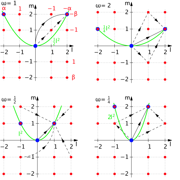
Figure 1: Schematic representation of the driving-induced transitions for driving frequencies $\omega=1/4,1/2,1,2$; see main text for the meaning of the various symbols. In each case the direct, first-order (solid arrows) and indirect, second-order (dashed arrows) transition amplitudes interfere to produce a ratchet current. For clarity, in the $\omega=1/2$ figure the first dashed arrow of the various second-order processes has been omitted.

In this peculiar $xy$ space all resonant states are “degenerate” with energy $\varepsilon_{lm}^{0}=0$. These states are connected by the driving (13), (19). By construction, our initial state corresponds to the unperturbed Floquet state $|00\rangle,$ where in general $|lm\rangle$ is the state characterized by $\vec{k}_{lm}$, its wave function being

$$\langle x,y|lm\rangle=\phi_{lm}^{0}(x,y)~{}.$$ (21)

This state $|00\rangle$ is represented by the filled blue circle in each of the four graphs of Fig. 1. Thus we expect the driving to mix $|00\rangle$ with the other resonant Floquet states satisfying $\varepsilon_{lm}^{0}=0$.

Let us focus first on the case $\omega=1$ (upper-left graph of Fig. 1). Starting from the state

$$\phi_{00}^{0}(x,y)=(2\pi T)^{-1/2}~{},$$ (22)

we expect the system to evolve from $|00\rangle$ towards $|22\rangle$ and $|\bar{2}2\rangle$, where $\bar{l}\equiv-l$. In general, under the effect of driving the state $|00\rangle$ will also mix with higher-lying unperturbed Floquet states, but we may expect that mixing to be weaker as it involves higher powers in the Fourier components $V_{\vec{g}}$, all of which are small because $K$ is assumed to be small. Thus a truncated Hilbert space spanned only by the Floquet states $\left\{|00\rangle,|22\rangle,|2\bar{2}\rangle\right\}$ may suffice to describe the dynamics under weak driving. The next section is devoted to the formulation of the three-level model.

IV Three-level model: effective matrix elements.

Inspection of the upper-left Fig. 1 strongly suggests that for $\omega=1$, the mixing between $|00\rangle$ and e.g. the state $|22\rangle$ must be dominated by the interference between the first-order process involving $\vec{g}=(2,2)$ once, and the the second-order process involving $\vec{g}=(1,1)$ twice (with $\vec{g}$ given in the units of the array there shown), while visiting the state $|11\rangle$ virtually. In this section we calculate the effective matrix elements which account for this first- and second-order mixing in an effective time-independent problem defined in the $xy$ space.

First we note that, in this $xy$ representation, we deal with a formally time-independent problem defined by the Hamiltonian

$$H=H_{0}+V~{},$$ (23)

where $H_{0}$ is given in (14) and $V$ by (13). The full Green function $G(z)\equiv(z-H)^{-1}$ can be related to its unperturbed counterpart $G^{0}(z)\equiv(z-H_{0})^{-1}$ through the Dyson equation economou

$$G=G^{0}+G^{0}VG~{}.$$ (24)

One may also describe the effect of the perturbation $V$ in terms of the $T$-matrix (not to be confused with the time-period) satisfying

$$T=V+VG^{0}T$$ (25)

or, equivalently,

$$G=G^{0}+G^{0}TG^{0}.$$ (26)

Thus the effective dynamics up to second order in $V$ may be described in terms of an effective $T$-matrix approximated as

$$T(z)\simeq V+VG^{0}(z)V~{}.$$ (27)

Finding the matrix elements of this approximate, second-order $T$-matrix is equivalent to finding those of an effective $\tilde{V}$ which, treated to first order, yields the correct second-order dynamics. So the next goal is to compute the matrix elements $\langle lm|T|l^{\prime}m^{\prime}\rangle.$ Applying the closure relation to (27) we obtain

$$\langle j|T(z)|j^{\prime}\rangle=\langle j|V|j^{\prime}\rangle+\sum_{j^{\prime\prime}}\frac{\langle j|V|j^{\prime\prime}\rangle\langle j^{\prime\prime}|V|j^{\prime}\rangle}{z-\varepsilon_{j^{\prime\prime}}^{0}}~{},$$ (28)

where $j$ is a short-hand notation for the quantum numbers $lm$.

For the case $\omega=1$ we restrict our analysis to the matrix elements between the three resonant states $\{|00\rangle,|22\rangle,|\bar{2}2\rangle\}$. These three states have an unperturbed energy $\varepsilon_{j}^{0}=0$, so in (28) we focus on the shell $z=0$. Inspection of Fig. 1 clearly shows that the intermediate state $|j^{\prime\prime}\rangle$ connecting $|00\rangle$ and $|22\rangle$ is $|11\rangle$, while $|\bar{1}1\rangle$ is the intermediary between $|00\rangle$ and $|\bar{2}2\rangle$. Thus, for example,

$$\langle 00|T|22\rangle = \langle 00|V|22\rangle-\frac{\langle 00|V|11\rangle\langle 11|V|22\rangle}{\varepsilon_{11}^{0}}=V_{22}-\frac{V_{11}^{2}}{\varepsilon_{11}^{0}}$$ (29)

$$= \frac{K}{4}\left(-\alpha\beta+\frac{K}{2}\right)\equiv\Gamma_{+}~{},$$

where $V_{lm}$ stands for the Fourier component $V_{\vec{g}}$, with $\vec{g}=(l,m)$ given in the units of Fig. 1.

Similarly,

$$\langle 00|T|\bar{2}2\rangle=\Gamma_{-}~{},$$ (30)

with

$$\Gamma_{\pm}=\frac{K}{4}\left(\mp\alpha\beta+\frac{K}{2}\right)~{}.$$ (31)

Restricting to these two well-behaved second-order matrix elements, we construct a three-level model defined by the Hamiltonian matrix

$$H_{3}\equiv\left[\begin{array}[]{ccc}0&\Gamma_{+}&0\\ \Gamma_{+}&0&\Gamma_{-}\\ 0&\Gamma_{-}&0\end{array}\right]~{},$$ (32)

spanning the space $\left\{|22\rangle,|00\rangle,|2\bar{2}\rangle\right\}$ or, for brevity, $\left\{|2\rangle,|0\rangle,|\bar{2}\rangle\right\}$ (using this ordering). In the subspace $\left\{|2\rangle,|\bar{2}\rangle\right\}$ it is always possible to introduce a rotation such that one state is decoupled from $|0\rangle$. Specifically, if we define the orthonormal states

$$|a\rangle = \frac{1}{\sqrt{\Gamma_{+}^{2}+\Gamma_{-}^{2}}}\left(\Gamma_{+}|2\rangle+\Gamma_{-}|\bar{2}\rangle\right)$$ (33)

$$|b\rangle = \frac{1}{\sqrt{\Gamma_{+}^{2}+\Gamma_{-}^{2}}}\left(\Gamma_{-}|2\rangle-\Gamma_{+}|\bar{2}\rangle\right)~{},$$ (34)

we find that $\langle 0|T|b\rangle=0,$ so that (32) transforms into

$$\tilde{H}_{3}=\left[\begin{array}[]{ccc}0&\Gamma&0\\ \Gamma&0&0\\ 0&0&0\end{array}\right]~{},$$ (35)

where

$$\Gamma=\langle 0|T|a\rangle=\sqrt{\Gamma_{+}^{2}+\Gamma_{-}^{2}}=\frac{K}{4\sqrt{2}}\sqrt{K^{2}+4\alpha^{2}\beta^{2}}~{}.$$ (36)

Therefore, for each particular driving the general three-level model can be truncated to an effective two-level problem, as found numerically in Ref. prl, .

V Averages of the current

Returning to the real time ($xt$) picture, it is clear that if the system is initially prepared in a given state $\psi(x,0)$, its subsequent evolution for $t>0$, when the driving is on [we assume (2) is multiplied by a step function $\theta(t)$], can be economically written as an expansion in the complete basis of the Floquet states, of general form (7)

$$\psi(x,t) = \sum_{j}c_{j}\exp(-i\varepsilon_{j}t)\phi_{j}(x,t)~{},$$ (37)

$$c_{j} = \int\phi_{j}(x,0)^{\ast}\psi(x,0)dx~{},$$ (38)

In this sense the Floquet states represent a generalization of the standard energy eigenstates of static Hamiltonians to the case of time-periodic systems.

Within our perturbative approach, we have seen that the three-level picture reduces in each case to a two-state ($|0\rangle$ and $|a\rangle$) problem, of Hamiltonian (35). Thus, if the initial state is $|\psi(0)\rangle=|0\rangle$, or $\psi(x,0)=(2\pi T)^{-1/2}$, the system will undergo a simple oscillation of the Rabi type between the unperturbed Floquet states $|0\rangle$ and $|a\rangle$. The frequency of those oscillations will be $2\Gamma$. Oscillations of exactly this type were observed in the numerical investigation of this model in Ref. prl, and in the recent experimental investigation bonn .

As well as evaluating the time-dependent current, it is also convenient to calculate the time-averaged current. This is particularly important to verify the existence of a long-lasting ratchet effect, which requires that the time-averaged current remains non-zero as the observation period tends to infinity. Such time-averages can be formed in two distinct ways. The first is the stroboscopic average, in which the current is evaluated only at discrete times $t_{n}=t_{0}+nT$, where $t_{0}\in\left(0,T\right]$. It can be defined as

$$\bar{I}_{s}(t_{0},N)\equiv\frac{1}{N}\sum_{n=0}^{N}I(t_{0}+nT)~{}.$$ (39)

This is frequently the scheme of measurement most convenient for experiment. One example is when the driving potential $V(x,t)$ is obtained by periodically accelerating and decelerating the optical lattice, thereby producing an inertial force in the rest frame of the lattice. Measurements of the current, however, are made in the rest frame of the laboratory, and so it is convenient to make measurements at times when the laboratory and lattice rest frames coincide, which occurs stroboscopically. The other averaging scheme is a continuous time average,

$$\bar{I}_{c}(\tau)\equiv\tau^{-1}\int_{0}^{\tau}I(t)dt~{}.$$ (40)

When the period of the driving is much shorter than the response of the system, these averages will coincide at long times. However, for lower driving frequencies it is possible that the two time-averages will yield different results, as the stroboscopic sampling will only capture a subset of the system’s dynamics.

At long times ($N,\tau\rightarrow\infty$), we can use (5), (37), (39), and (40) to write these time-averaged currents as

$$\bar{I}_{s}(t_{0}) = \sum_{j}|c_{j}|^{2}\langle\phi_{j}(t_{0})|p_{x}|\phi_{j}(t_{0})\rangle~{},$$ (41)

$$\bar{I}_{c} = \frac{1}{T}\int_{0}^{T}dt_{0}\,\bar{I}_{s}(t_{0})\;.$$ (42)

In (41) we have assumed that $\varepsilon_{j}\neq\varepsilon_{j^{\prime}}$ for all $j\neq j^{\prime}$.

Once the driving has been switched on and Rabi oscillations have started, the system will spend, on average, half its time in $|0\rangle$ and $|a\rangle$. Thus the analytical prediction for the ratchet current is simply ($I\equiv\bar{I}_{c}$)

$$I=I_{a}/2~{},$$ (43)

where  $I_{a}\equiv\langle a|p_{x}|a\rangle$ is the current carried by $|a\rangle$.

We first consider the case of the main resonance $\omega=1$. In this case the Rabi oscillation occurs between $|0\rangle$ and $|a\rangle$ given by (33), with frequency

$$\Omega_{R}=2\Gamma=\frac{K}{2\sqrt{2}}\sqrt{K^{2}+4\alpha^{2}\beta^{2}}~{}.$$ (44)

We note that, in our reduced units, the states $|2\rangle$ and $|\bar{2}\rangle$, carry currents 2 and -2, respectively. As a result, the ratchet current can be shown to be

$$I=\frac{4K\alpha\beta}{K^{2}+4\alpha^{2}\beta^{2}}~{}.$$ (45)

From (45) the beautiful picture emerges of a coherent ratchet current stemming from the interference between first- and second-order processes creating an imbalance between the matrix elements coupling the initial, time-symmetric state $|0\rangle$ to the current-carrying states $|2\rangle$ and $|\bar{2}\rangle$. Most importantly, the ratchet current exists only if both $\alpha$ and $\beta$ are nonzero, i.e. if the driving is both space- and time-asymmetric, in agreement with the symmetry analysis provided in denisov . We can further observe that the ratchet current is a unique function of the product $\alpha\beta$, and for this driving frequency the ratchet current is maximized for $\alpha\beta=K/2$, in excellent agreement with the experimental observation bonn .

Figure 2 shows the extremely good agreement between the analytical prediction of the three-level model and the full numerical simulation for the time-dependent ratchet current in the weak coupling case ($K=0.1$). In particular, this means that the analytical predictions (44) and (45) for the Rabi frequency and the long-time ratchet current become essentially exact in the weak-driving limit. As expected, the agreement with the perturbative analytical calculation worsens for higher $K$.

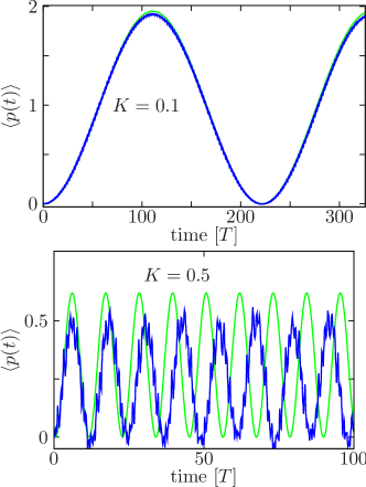
Figure 2: Comparison of the time-dependent current predicted by the effective three-level model and the exact numerical results, for $\omega=1$ and asymmetry parameters $\alpha=\beta=0.2$. The three-level model predicts Rabi oscillations which fit the exact results extremely well for weak driving ($K=0.1$). For strong driving ($K=0.5$) the exact results show additional small, high-frequency oscillations, but the main behavior is still reasonably well-described by the effective model.

We recall that our analysis predicts, in addition to the main resonance at $\omega=1$, additional resonances for $\omega=1/4,1/2,\mbox{ \ and \ }2$. To verify this prediction we show in Fig. 3 the time-averaged current obtained for a fixed driving strength of $K=0.05$ as the frequency is varied over a wide range. We can first note that we indeed see peaks at the four resonant frequencies indicated by our model. A similar set of resonance peaks was observed in the experimental investigation of this ratchet bonn . The $\omega=1$ peak is considerably larger than the others, and it is interesting to note that the response for $\omega=1/2$ is of opposite sign to the other peaks. This peak is also unusual in its sensitivity to the averaging procedure used; the stroboscopic result is larger and broader than the continuous time-average. In the inset we show an enlargement of the small-scale structure in the current response, which indicates the existence of further families of sub-resonant peaks, of much smaller magnitude than the four primary peaks, occurring at commensurate fractions of the driving frequencies. This perhaps indicates the role of higher order interference processes, which could in principle be described by a suitable generalization of our procedure.

Figure 3: Time-averaged current, averaged over 4000 driving periods for a weakly-driven system ($K=0.05$, asymmetry parameters $\alpha=\beta=0.2$), plotted as a function of the driving frequency. Four peaks appear, at driving frequencies of $\omega=0.25,0.5,1,2$ in agreement with the resonant condition (18). Inset: Magnified view, showing the existence of sub-resonances at commensurate fractions of the resonant frequencies. We also note the reduction of the $\omega=0.5$ resonance when the time-average is evaluated continuously instead of stroboscopically.

In the same way as for the $\omega=1$ resonance, we can obtain analytical results for the ratchet currents produced by the other main resonances, governed by first and second order transitions as indicated in Fig. 1. These results are given in Table 1. In Fig. 4 we compare the analytical and numerical predictions for the continuously time-averaged ratchet current for the four main resonances. The agreement is excellent. We note in particular the linear behavior $I\propto K$ for small $K,$ which is also predicted analytically, and the existence of a maximum current for $\omega=1$, occurring for a driving strength of $K=0.08$.

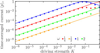
Figure 4: Comparison of the analytical results with numerically-exact data for the four principal resonances, $\omega=0.25,0.5,1,2$ 8 (see Table I). The values for $\omega=\frac{1}{2}$ are actually negative, and so for convenience we plot their absolute value. For all the curves the asymmetry parameters were set to be $\alpha=\beta=0.2$. We can see that for weak driving strengths the agreement is excellent; the effective three-level model produces quantitatively accurate results. For higher driving strengths the model diverges from the exact results, as expected for a perturbative result.

As well as the amplitude of the ratchet current, the effective model also provides predictions for the period of the Rabi oscillations. In Fig. 5 we compare these predictions [see Eq. (44)] with the numerically exact results, and again see excellent, quantitative agreement over a wide range of driving amplitudes.

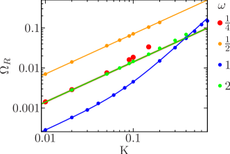
Figure 5: Rabi frequencies, $\Omega_{R}$, predicted by the effective three-level model [see Eq. (44) and Table 1] are shown with solid lines, to compare with data extracted from numerically exact simulations. As in Fig. 4, we see excellent agreement between analytics and numerics.

Finally, in Fig. 6 we show the stroboscopically-averaged current as a function of the initial sampling point time $t_{0}$. For $\omega=0.25,1,\mbox{ \ and \ }2$ the stroboscopic quantity shows only a very weak dependence on $t_{0}$. The $\omega=0.5$ resonance, however, does display an important dependence on $t_{0}$, and indeed changes sign as $t_{0}$ varies over the range $0\leq t_{0}\leq T$. This causes the continuously-averaged current to be significantly smaller than a stroboscopic estimate for this driving frequency [see Eq. (42)], as can be seen in Fig. 3.

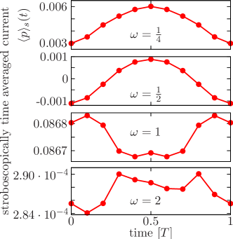
Figure 6: The stroboscopic average is evaluated at discrete times $t_{n}=t_{0}+nT$. Here we show the dependence of this time average on the initial time sampling point $t_{0}$. For $\omega=0.25,1,2$ the variation is weak, but for $\omega=0.5$ the dependence is strong, and contributes to the low value of the continuous current average for this value of the driving frequency. The number of driving periods used to compute the stroboscopic average is, from top to bottom, 400, 400, 600, 300. This amounts to about ten complete Rabi periods ($2\pi/\Omega_{R}$) in the first two cases, and one Rabi period in the last two.

aa$\omega$aa	$\Omega_{R}$	$I$
$\frac{1}{4}$	$\frac{K}{\sqrt{2}}\left[(\frac{4}{7}K\alpha)^{2}+\beta^{2}\right]^{1/2}$	$\frac{56K\alpha\beta}{7\beta^{2}+16(K\alpha)^{2}}$
$\frac{1}{2}$	a$\frac{K}{\sqrt{2}}\left[1+(\frac{1}{10}K\alpha\beta)^{2}\right]^{1/2}$a	$-\frac{10K\alpha\beta}{(K\alpha\beta)^{2}+100}$
$1$	$\frac{K}{2\sqrt{2}}\left[K^{2}+(2\alpha\beta)^{2}\right]^{1/2}$	$\frac{4K\alpha\beta}{K^{2}+(2\alpha\beta)^{2}}$
$2$	$\frac{K}{\sqrt{2}}\left[(\frac{1}{35}K\beta)^{2}+\alpha^{2}\right]^{1/2}$	$\frac{70K\alpha\beta}{(35\alpha)^{2}+(K\beta)^{2}}$

Table 1: Analytic results for the Rabi frequencies and the continuously time-averaged ratchet currents for the four resonant frequencies considered.

VI Conclusions

We have studied an unusual form of flashing ratchet, in which the spatial and time symmetries can be controlled independently. Using a novel form of perturbation theory, we find that we are able to describe the weak-driving regime of this system to a surprisingly high degree of accuracy by using a three-level effective model, which later reduces, in each particular case, to a simple two-level model. This provides an analytical underpinning to the phenomenological two-level model introduced in Ref. prl, to describe this ratchet system. The ratchet current arises from the interference between first- and second-order driving-induced processes, and so is a purely quantum coherent effect, not involving dissipation. It should be noted that we have neglected the effect of the non-linear interaction $g$. In Ref. prl, it was shown that this has the effect of damping the Rabi oscillations, eventually producing a “self-trapped” state. Introducing the non-linearity in a consistent way to this model remains a interesting topic for future work.

Acknowledgments. This work was supported by MICINN (Spain), through grant FIS-2007-65723 and the Ramón y Cajal Program (CEC).

References

- (1) P. Reimann, Phys. Rep. 361, 57 (2002).
- (2) P. Hänggi and F. Marchesoni, Rev. Mod. Phys. 81, 387 (2009).
- (3) S. Flach, O. Yevtushenko, and Y. Zolotaryuk, Phys. Rev. Lett. 84, 2358 (2000).
- (4) H. Schanz, M.-F. Otto, R. Ketzmerick, and T. Dittrich, Phys. Rev. Lett. 87, 070601 (2001).
- (5) G. Hur, C.E. Creffield, P.H. Jones, and T.S. Monteiro, Phys. Rev. A 72, 013403 (2005).
- (6) J. Gong and P. Brumer, Phys. Rev. Lett. 97, 240602 (2006).
- (7) M. Sadgrove, M. Horikoshi, T. Sekimura, and K. Nakagawa, Phys. Rev. Lett. 99 043002 (2007); I. Dana, V. Ramareddy, I. Talukdar, and G. S. Summy, Phys. Rev. Lett. 100, 024103 (2008).
- (8) D. Poletti, G. Benenti, G. Casati and B. Li, Phys. Rev. A 76, 023421 (2007).
- (9) D. Poletti, G. Benenti, G. Casati, P. Hänggi, and B. Li, Phys. Rev. Lett. 102, 1300604 (2009).
- (10) C.E. Creffield and F. Sols, Phys. Rev. Lett 103, 200601 (2009).
- (11) R. Gommers, S. Bergamini, and F. Renzoni, Phys. Rev. Lett. 95, 073003 (2005).
- (12) R. Bartussek, P. Hänggi and J.G. Kissner Europhys. Lett. 28 459 (1994).
- (13) T. Salger, S. Kling, T. Hecking, C. Geckeler, L. Morales-Molina, and M. Weitz, Science 326, 1241 (2009).
- (14) E. N. Economou, Green’s Functions in Quantum Physics, 3rd Edition (Springer, Berlin, 2006).
- (15) S. Denisov, L. Morales-Molina, S. Flach, and P. Hänggi, Phys. Rev. A 75, 063424 (2007).