An empirical Bayes procedure for the selection of Gaussian graphical models

Abstract

A new methodology for model determination in decomposable graphical Gaussian models (Dawid and Lauritzen,, 1993) is developed. The Bayesian paradigm is used and, for each given graph, a hyper inverse Wishart prior distribution on the covariance matrix is considered. This prior distribution depends on hyper-parameters.
It is well-known that the models’s posterior distribution is sensitive to the specification of these hyper-parameters and no completely satisfactory method is registered. In order to avoid this problem, we suggest adopting an empirical Bayes strategy, that is a strategy for which the values of the hyper-parameters are determined using the data. Typically, the hyper-parameters are fixed to their maximum likelihood estimations. In order to calculate these maximum likelihood estimations, we suggest a Markov chain Monte Carlo version of the Stochastic Approximation EM algorithm.
Moreover, we introduce a new sampling scheme in the space of graphs that improves the add and delete proposal of Armstrong et al., (2009). We illustrate the efficiency of this new scheme on simulated and real datasets.

Keywords: Gaussian graphical models, decomposable models, empirical Bayes, Stochastic Approximation EM, Markov Chain Monte Carlo

1 Gaussian graphical models in a Bayesian Context

Statistical applications in genetics, sociology, biology , etc often lead to complicated interaction patterns between variables. Graphical models have proved to be powerful tools to represent the conditional independence structure of a multivariate distribution : the nodes represent the variables and the absence of an edge between two vertices indicates some conditional independence between the associated variables.

Our paper presents a new approach for estimating the graph structure in Gaussian graphical model. A very large literature deals with this issue in the Bayesian paradigm: Dawid and Lauritzen, (1993); Madigan and Raftery, (1994); Giudici and Green, (1999); Jones et al., (2005); Armstrong et al., (2009); Carvalho and Scott, (2009). For a frequentist point of view, one can see Drton and Perlman, (2004).

We suggest here an empirical Bayes approach: the parameter of the prior are estimated from the data. Parametric empirical Bayes methods have a long history, with major developments evolving in the sequence of papers by Efron and Morris, (1971); Efron and Morris, 1972b ; Efron and Morris, 1972a ; Efron and Morris, 1973a ; Efron and Morris, 1973b ; Efron and Morris, 1976b ; Efron and Morris, 1976a . Empirical Bayes estimation falls outside the Bayesian paradigm. However, it has proven to be an effective technique of constructing estimators that performs well under both Bayesian and frequentist criteria. Moreover, in the case of decomposable Gaussian graphical models, it gives a default and objective way for constructing prior distribution. The theory and applications of empirical Bayes methods are given by Morris, (1983).

In this Section, we first recall some results on Gaussian graphical models, then we justify the use of the empirical Bayes strategy.

1.1 Background on Gaussian graphical models

Let $\mathcal{G}=(V,E)$ be an undirected graph with vertices $V=\{1,\ldots,p\}$ and set of edges
$E=$ $\{e_{1},\ldots,e_{t}\}$, ($\forall i=1,\ldots,t$, $e_{i}\in V\times V$). Using the notations of Giudici and Green, (1999), we first recall the definition of a decomposable graph. A graph or subgraph is said to be complete if all pairs of its vertices are joined by edges. Moreover, a complete subgraph that is not contained within another complete subgraph is called a clique. Let $\mathcal{C}=\{C_{1},\ldots,C_{k}\}$ be the set of the cliques of an undirected graph.
An order of the cliques $(C_{1},\ldots,C_{k})$ is said to be perfect if $\forall i=2,\ldots,k$, $\exists h=h(i)\in\{1,\ldots,i-1\}$ such that $S_{i}=C_{i}\cap\cup_{j=1}^{i-1}C_{i}\subseteq C_{h}$. $\mathcal{S}=\{S_{2},\ldots,S_{k}\}$ is the set of separators associated to the perfect order $\{C_{1},\ldots,C_{k}\}$. An undirected graph admitting a perfect order is said to be decomposable. Let $\mathcal{D}_{p}$ denote the set of decomposable graphs with $p$ vertices. For more details, one can refer to Dawid and Lauritzen, (1993), Lauritzen, (1996) (Chapters 2, 3 and 5) or Giudici and Green, (1999).

The graph drawn in Figure 1 – and used as benchmark in numerical Section 4.2– is decomposable. Indeed, the set of cliques $C_{1}=\{1,2,3\}$, $C_{2}=\{2,3,5,6\}$, $C_{3}=\{2,4,5\}$, $C_{4}=\{5,6,7\}$ and $C_{5}=\{6,7,8,9\}$ with associated separators $S_{2}=\{2,3\}$, $S_{3}=\{2,5\}$, $S_{4}=\{5,6\}$ and $S_{5}=\{6,7\}$ forms a perfect order.

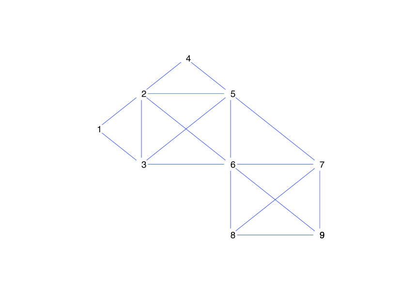
Figure 1: Example of decomposable graph

Note that, with $p$ vertices, the total number of possible graphs is $2^{p(p-1)/2}$, $p(p-1)/2$ being the number of possible edges. The total number of decomposable graphs with $p$ vertices can be calculated for moderate values of $p$. For instance, if $p=6$, among the $32\,768$ possible graphs, $18\,154$ are decomposable (around $55\%$); if $p=8$, then $30\,888\,596$ of the $268\,435\,456$ possible graphs are decomposable (around $12\%$).

A pair $(A,B)$ of subsets of the vertex set $V$ of an undirected graph $\mathcal{G}$ is said to form a decomposition of $\mathcal{G}$ if (1) $V=A\cup B$ , (2) $A\cap B$ is complete and (3) $A\cap B$ separates $A$ from $B$ ie any path from a vertex in $A$ to a vertex in $B$ goes through $A\cap B$.

To each vertex $v\in V$, we associate a random variable $y_{v}$. For $A\subseteq V$, $\mathbf{y}_{A}$ denotes the collection of random variables $\{y_{v}:v\in A\}$. To simplify the notation, we set $\mathbf{y}=\mathbf{y}_{V}$. The probability distribution of $\mathbf{y}$ is said to be Markov with respect to $\mathcal{G}$, if for any decomposition $(A,B)$ of $\mathcal{G}$, $\mathbf{y}_{A}$ is independent of $\mathbf{y}_{B}$ given $\mathbf{y}_{A\cap B}$. A graphical model is a family of distributions on $\mathbf{y}$ verifying the Markov property with respect to a graph.

A Gaussian graphical model, also called covariance selection model (see Dempster, (1972)), is such that

$$\mathbf{y}|\mathcal{G},\Sigma_{\mathcal{G}}\sim\mathcal{N}_{p}\left(\boldsymbol{\mu},\Sigma_{\mathcal{G}}\right)\,,$$ (1)

where $\mathcal{N}_{p}\left(\boldsymbol{\mu},\Sigma_{\mathcal{G}}\right)$ denotes the $p$-variate Gaussian distribution with expectation $\boldsymbol{\mu}\in\mathbb{R}^{p}$ and $p\times p$ symmetric definite positive covariance matrix $\Sigma_{\mathcal{G}}$. $\Sigma_{\mathcal{G}}$ has to ensure the Markov property with respect to $\mathcal{G}$. In the Gaussian case, $\mathbf{y}$ is Markov with respect to $\mathcal{G}=(V,E)$ if and only if

$$(i,j)\notin E\Longleftrightarrow\left(\Sigma_{\mathcal{G}}^{-1}\right)_{(i,j)}=0\,,$$

where $A^{-1}$ denotes the inverse of the matrix $A$. $\Sigma_{\mathcal{G}}^{-1}$ is called the concentration matrix.

In the following, we suppose that we observe a sample $\mathbf{Y}=(\mathbf{y}^{1},\ldots,\mathbf{y}^{n})$ from model (1) with mean parameter $\boldsymbol{\mu}$ set to zero. The data are expressed as a deviation from the sample mean. This centering strategy is standard in the literature, however the technique developed here can be easily extended to the case $\boldsymbol{\mu}\neq\mathbf{0}_{p}$.

The density of $\mathbf{Y}$ is a function of multivariate Gaussian densities on the cliques and separators of $\mathcal{G}$. More precisely, let $\mathcal{C}$ and $\mathcal{S}$ denote respectively the sets of the cliques and separators of $\mathcal{G}$ corresponding to a perfect order for $\mathcal{G}$. We have :

$$f(\mathbf{Y}|\Sigma_{\mathcal{G}},\mathcal{G})=\prod_{i=1}^{n}\left\{\frac{\prod_{C\in\mathcal{C}}\phi_{|C|}\left(\mathbf{y}^{i}_{C}|(\Sigma_{\mathcal{G}})_{C}\right)}{\prod_{S\in\mathcal{S}}\phi_{|S|}\left(\mathbf{y}^{i}_{S}|(\Sigma_{\mathcal{G}})_{S}\right)}\right\}\,,$$ (2)

where for every subset of vertices $A$, $|A|$ denotes its cardinal and $(\Sigma_{\mathcal{G}})_{A}$ is the restriction of $(\Sigma_{\mathcal{G}})$ to $A$ i.e. $\left\{(\Sigma_{\mathcal{G}})_{i,j}\right\}_{i\in A,j\in A}$ and $\mathbf{y}_{A}=(\mathbf{y}_{j})_{j\in A}$. $\phi_{q}\left(\cdot|\Delta\right)$ is the $q$-variate Gaussian density with mean $\mathbf{0}_{q}$ and $q\times q$ symmetric definite positive covariance matrix $\Delta$.

From a Bayesian perspective, we are interested in the posterior probabilities

$$\pi(\mathcal{G}|\mathbf{Y})\propto\pi(\mathcal{G})\int f(\mathbf{Y}|\Sigma_{\mathcal{G}},\mathcal{G})\pi(\Sigma_{\mathcal{G}}|\mathcal{G})d\Sigma_{\mathcal{G}}\,,$$ (3)

for specific priors $\pi(\Sigma_{\mathcal{G}}|\mathcal{G})$ and $\pi(\mathcal{G})$. In the following, we discuss the choice of these prior distributions.

1.2 Prior distributions specification

Prior and posterior distributions for the covariance matrix

 

Conditionally on $\mathcal{G}$, we set an Hyper-Inverse Wishart (HIW) distribution as prior distribution on $\Sigma_{\mathcal{G}}$:

$$\Sigma_{\mathcal{G}}|\mathcal{G},\delta,\Phi\sim\mbox{HIW}_{\mathcal{G}}\left(\delta,\Phi\right)\,,$$

where $\delta>0$ is the degree of freedom and $\Phi$ is a $p\times p$ symmetric positive definite location matrix. This distribution is the unique hyper-Markov distribution such that, for every clique $C\in\mathcal{C}$, $(\Sigma_{\mathcal{G}})_{C}\sim IW(\delta,\Phi_{C})$ with density

$$\begin{array}[]{ccl}\pi\left((\Sigma_{\mathcal{G}})_{C}|\delta,\Phi_{C}\right)&=&h^{IW}_{\mathcal{G}_{C}}(\delta,\Phi_{C})\left[\det(\Sigma_{\mathcal{G}})_{C}\right]^{-\frac{\delta+2|C|}{2}}\\ &&\exp\left\{-\frac{1}{2}\text{tr}\left[(\Sigma_{\mathcal{G}})_{C}^{-1}\Phi_{C}\right]\right\}\,,\\ \end{array}$$ (4)

where $h^{IW}_{\mathcal{G}_{C}}(\delta,\Phi_{C})$ is the normalizing constant:

$$h^{IW}_{\mathcal{G}_{C}}(\delta,\Phi_{C})=\frac{\det\left(\frac{\Phi_{C}}{2}\right)^{(|C|+\delta-1)/2}}{\Gamma_{|C|}\left(\frac{|C|+\delta-1}{2}\right)}\,,$$ (5)

where $\det(\cdot)$ and $\text{tr}(\cdot)$ are respectively the determinant and trace and $\Gamma_{v}$ is the multivariate $\Gamma$-function with parameter $v$:

$$\Gamma_{v}(a)=\pi^{v(v-1)/4}\prod_{j=1}^{v}\Gamma[a+(1-j)/2]\,.$$

The full joint density is:

$$\pi(\Sigma_{\mathcal{G}}|\mathcal{G},\delta,\phi)=\frac{\prod_{C\in\mathcal{C}}\pi\left((\Sigma_{\mathcal{G}})_{C}|\delta,\Phi_{C}\right)}{\prod_{S\in\mathcal{S}}\pi\left((\Sigma_{\mathcal{G}})_{S}|\delta,\Phi_{S}\right)}\,.$$ (6)

Conditionally on $\mathcal{G}$, the HIW distribution is conjugate. The posterior distribution of $\Sigma_{\mathcal{G}}$ is given by (Giudici,, 1996):

$$\Sigma_{\mathcal{G}}|\mathbf{Y},\mathcal{G},\delta,\Phi\sim\mbox{HIW}\left(\delta+n,\Phi+S_{\mathbf{Y}}\right)\,.$$ (7)

where $S_{\mathbf{Y}}=\sum_{i=1}^{n}\mathbf{y}^{i}\>\mathstrut{}^{t}\mathbf{y}^{i}$, $\mathstrut{}^{t}v$ denoting the transpose of $v$.

Moreover for such a prior distribution, the marginal likelihood for any graph $\mathcal{G}$ is a simple function of the HIW prior and posterior normalizing constants $h_{\mathcal{G}}(\delta,\Phi)$ and $h_{\mathcal{G}}(\delta+n,\Phi+S_{\mathbf{Y}})$ (Giudici,, 1996):

$$f(\mathbf{Y}|\mathcal{G},\delta,\Phi)=\frac{h_{\mathcal{G}}(\delta,\Phi)}{(2\pi)^{-np/2}h_{\mathcal{G}}(\delta+n,\Phi+S_{\mathbf{Y}})}\,.$$ (8)

where $h_{\mathcal{G}}(\delta,\Phi)$ is the normalizing constant of the HIW distribution which can be computed explicitly in decomposable graphs from the normalizing constants of the inverse Wishart cliques and separators densities (4-5-6) :

$$\begin{array}[]{ccc}h_{\mathcal{G}}(\delta,\Phi)&=&\frac{\prod_{C\in\mathcal{C}}h^{IW}_{\mathcal{G}_{C}}(\delta,\Phi_{C})}{\prod_{S\in\mathcal{S}}h^{IW}_{\mathcal{G}_{S}}(\delta,\Phi_{S})}\,.\end{array}$$

Note that Roverato, (2002) extends the Hyper-Inverse Wishart distribution to non- decomposable cases. Moreover, a general treatment of priors for decomposable models is given by Letac and Massam, (2007).

Prior and posterior distributions for the graphs

 

The prior distribution in the space of decomposable graphs has been widely discussed in the literature. The naive choice is to use the standard uniform prior distribution:

$$\pi(\mathcal{G})\propto 1\,.$$

One great advantage of this choice is simplifying the calculus but it can be criticized. Indeed, with $p$ vertices, the number of possible edges is equal to $m=\frac{p(p-1)}{2}$ and, in the case of a uniform prior over all graphs, the prior number of edges has its mode around $m/2$ which is typically too large.

An alternative to this prior is to set a Bernouilli distribution of parameter $r$ on the inclusion or not of each edge (Jones et al.,, 2005; Carvalho and Scott,, 2009)

$$\pi(\mathcal{G}|r)\propto r^{k_{\mathcal{G}}}(1-r)^{m-k_{\mathcal{G}}}\,,$$ (9)

where $k_{\mathcal{G}}$ is the number of edges of $\mathcal{G}$. The parameter $r$ has to be calibrate. If $r=1/2$, this prior resumes to the uniform one.

In the following we consider this prior distribution and give an empirical estimation of $r$.

Using (8) and (9), we deduce easily that the density of the posterior distribution in the space of decomposable graphs satisfies:

$$\pi\left(\mathcal{G}|\mathbf{Y},\delta,r,\Phi\right)\propto\frac{h_{\mathcal{G}}(\delta,\Phi)}{h_{\mathcal{G}}(\delta+n,\Phi+S_{\mathbf{Y}})}\pi(\mathcal{G}|r)\,.$$ (10)

This posterior distribution is known to be sensitive to the specification of the hyper-parameters $r$, $\delta$ and $\Phi$ (see Jones et al., (2005); Armstrong et al., (2009)). To tackle this problem various strategies have been developed. In the following, we supply a short review of these methods and offer an alternative one.

Choice of the hyper-parameters $\delta$, $r$ and $\Phi$

 

In a fully Bayesian context, as proposed by Giudici and Green, (1999), a hierarchical prior modelling can be used. In this approach, $\delta$and $\Phi$ are considered as random quantities and a prior distribution is assigned to those parameters ($r$ is fixed to $1/2$). This strategy does not completely solve the problem since the prior distributions on $\delta$ and $\Phi$ also depend on hyper-parameters which are difficult to calibrate.

An other strategy consists in fixing the values of $\delta$, $r$ and $\Phi$ as in Jones et al., (2005). In that paper, $r$ is set to $\frac{1}{p-1}$ encouraging sparse graphs. They choose $\delta=3$ which is the minimal integer such that the first moment of the prior distribution on $\Sigma_{\mathcal{G}}$ exists. Finally, they set $\Phi=\tau I_{p}$ and using the fact that the mode of the marginal prior for each variance terms $\sigma_{ii}$ is equal to $\tau/(\delta+2)$, $\tau$ is fixed to $\delta+2$ if the data set is standardized.

An intermediate strategy is suggested by Armstrong et al., (2009). First, they fix the value of $\delta$ to $4$ assessing that such a value gives a suitably non-informative prior for $\Sigma_{\mathcal{G}}$. Then, they consider different possibilities for $\Phi$, all of the form $\Phi=\tau A$ where the matrix $A$ is fixed. In all cases, for the hyper-parameter $\tau$, they use a uniform prior distribution on the interval $[0,\Gamma]$ where $\Gamma$ is very large. Finally, they also use a hierarchical prior on $r$ : $r\sim\beta(1,1)$, which leads to

$$\pi(G)\propto\left(\begin{array}[]{c}m\\ k_{\mathcal{G}}\end{array}\right)^{-1}$$

by integration. $\left(\begin{array}[]{c}m\\ k_{\mathcal{G}}\end{array}\right)$ is the binomial coefficient.

This hierarchical prior of $r$ is also used in Carvalho and Scott, (2009). In that paper, they suggest a HIW $g$-prior approach with $g=1/n$. This approach consists of fixing $\delta=1$ and $\Phi=S_{\mathbf{Y}}/n$.

In our point of view, $\delta$ measures the amount of information in the prior relative to the sample (see (7)): we suggest setting $\delta$ to $1$ such that the prior weight is the same as the weight of one observation. As pointed out by Jones et al., (2005), for this particular choice, the first moment of the prior distribution on $\Sigma_{\mathcal{G}}$ does not exist. However, for $\delta=1$, the prior distribution is proper and we fail to see any argument in favour of the existence of a first moment.

The structure of $\Phi$ can be discussed and various forms exist in the literature (see Armstrong et al., (2009) for instance). In this paper, we standardise the data and use $\Phi=\tau I_{p}$. This choice leads to sparse graph: on average each variable has major interactions with a relatively small number of other variables. In that context, $\tau$ plays the role of a shrinkage factor and has to be carefully chosen on the appropriate scale.

In this paper, we recommend to use an empirical Bayes strategy and to fix $(\tau,r)$ to its maximum likelihood estimation for which computation is a challenging issue. To tackle this point, a Markov Chain Monte Carlo (MCMC) version of the Stochastic Approximation EM (SAEM) algorithm is used.

The SAEM algorithm is presented in Section 2. In Section 3, a new Metropolis-Hasting algorithm is introduced. Then, the proposed methodology is tested on real and simulated datasets.

2 An empirical Bayes procedure via the SAEM-MCMC algorithm

In the following, we set $\theta=(\tau,r)\in\mathbb{R}^{*+}\times]0,1[$. In order to compute the maximum likelihood estimation of $\theta$, we need to optimize in $\theta$ the following function

$$f(\mathbf{Y}|\theta)\propto\sum_{\mathcal{G}\in\mathcal{D}_{p}}\left\{\frac{h_{\mathcal{G}}(\delta,\tau I_{p})}{h_{\mathcal{G}}(n+\delta,\tau I_{p}+S_{\mathbf{Y}})}\right\}\pi(\mathcal{G}|r)\,$$ (11)

If the number of vertices is greater than $10$, the number of decomposable graphs is so huge that it is not possible to calculate the sum over $\mathcal{D}_{p}$. In that case, we consider the use of the Expectation-Maximization (EM) algorithm developed by
Dempster et al., (1977), noting the fact that the data $\mathbf{Y}=$
$(\mathbf{y}^{1},\ldots,\mathbf{y}^{n})$ are issued from the partial observations of the complete data $(\mathbf{Y},\mathcal{G},\Sigma_{\mathcal{G}})$. However, for such a data augmentation scheme, the E-step of the EM algorithm is not explicit and we have to resort to a stochastic version of the EM algorithm, like:

1. the S-EM scheme introduced by Celeux and Diebolt, (1992) and Diebolt and Celeux, (1993) where the E-step is replaced by a single simulation from the distribution of $(\mathcal{G},\Sigma_{\mathcal{G}})$ given $\mathbf{Y}$ and $\theta$;

2. the MC-EM or the MCMC-EM algorithms
   where the E-step is replaced by some Monte Carlo approximations
   (McLachlan and Krishnan,, 2008);

3. the SAEM algorithm introduced by Delyon et al., (1999) where the E-step is divided into a simulation step and a stochastic approximation step;

4. the SAEM-MCMC algorithm
   (Kuhn and Lavielle,, 2004) which extends the SAEM scheme, the “exact” simulation step being replaced by a simulation from an ergodic Markov chain.

The S-EM, MC-EM and SAEM methods require to simulate a realization from the distribution of $(\mathcal{G},\Sigma_{\mathcal{G}})$ given $\mathbf{Y}$ and $\theta$. We are not able to produce a realization exactly distributed from the distribution of $(\mathcal{G},\Sigma_{\mathcal{G}})$ given $\mathbf{Y}$ and $\theta$. We use the SAEM-MCMC algorithm which just requires some realizations from an ergodic Markov chain with stationary distribution $(\mathcal{G},\Sigma_{\mathcal{G}})|\mathbf{Y},\theta$. In a first part, we recall the EM algorithm principles and present the SAEM-MCMC scheme. In a second part, we detail its application to Gaussian graphical models and prove its convergence.

2.1 The Stochastic Approximation version of the EM algorithm

The EM algorithm is competitive when the maximization of the function

$$\theta\rightarrow Q(\theta|\theta^{\prime})=\mathbb{E}_{\Sigma_{\mathcal{G}},\mathcal{G}|\mathbf{Y},\theta^{\prime}}\left\{\log f(\mathbf{Y},\Sigma_{\mathcal{G}},\mathcal{G}|\theta)\right\}$$

is easier than the direct maximization of the marginal likelihood (11). The EM algorithm is a two steps iterative procedure. More precisely, at the $k$-th iteration, the E-step consists of evaluating $Q_{k}(\theta)=Q(\theta\,|\,\widehat{\theta}_{k-1})$ while the M-step updates $\widehat{\theta}_{k-1}$ by maximizing $Q_{k}(\theta)$.

For complicated models where the E-step is untractable, Delyon et al., (1999) introduce the Stochastic Approximation EM algorithm (SAEM) replacing the E-step by a stochastic approximation of $Q_{k}(\theta)$. At iteration $k$, the E-step is divided into a simulation step (S-step) of $\left(\Sigma_{\mathcal{G}}^{(k)},\mathcal{G}^{(k)}\right)$ with the posterior distribution $(\Sigma_{\mathcal{G}},\mathcal{G})|\mathbf{Y},\widehat{\theta}_{k-1}$ and a stochastic approximation step (SA-step):

$$\begin{array}[]{cll}Q_{k}(\theta)&=&(1-\gamma_{k})Q_{k-1}(\theta)+\\ &&\gamma_{k}\log f(\mathbf{Y},\Sigma_{\mathcal{G}}^{(k)},\mathcal{G}^{(k)}|\widehat{\theta}_{k-1})\end{array}$$

where $(\gamma_{k})_{k\in\mathbb{N}}$ is a sequence of positive numbers decreasing to zero. When the joint distribution of $(\mathbf{Y},\Sigma_{\mathcal{G}},\mathcal{G})$ belongs to the exponential family, the SA-step reduces to the stochastic approximation on the minimal exhaustive statistics. The M-step remains the same. One of the benefits of the SAEM algorithm is the low-level dependence on the initialization $\theta_{0}$, due to the stochastic approximation of the SA-step.

In Gaussian graphical models, we cannot generate directly a realization from the conditional distribution of $(\Sigma_{\mathcal{G}},\mathcal{G})$ given $\mathbf{Y}$ and $\widehat{\theta}_{k-1}$. For such cases, Kuhn and Lavielle, (2004) suggest to replace the simulation step by a MCMC scheme which consists of generating $M$ realizations from an ergodic Markov chain with stationary distribution $\Sigma_{\mathcal{G}},\mathcal{G}|\mathbf{Y},\widehat{\theta}_{k-1}$ and use the last simulation in the SAEM algorithm. Kuhn and Lavielle, (2004) prove the convergence of the estimates sequence provided by this SAEM-MCMC algorithm towards a maximum of the function $f(\mathbf{Y}|\theta)$ under general conditions for the exponential family.

2.2 The SAEM-MCMC algorithm on Gaussian graphical models

In this section, we detail the application of the SAEM-MCMC algorithm to the Gaussian graphical model introduced in Section 1.2. More precisely, we give the expression of the complete log-likelihood and of the minimal sufficient statistics. Lavielle and Lebarbier, (2001) applied the same methodology on a change-point problem.

The complete log-likelihood $f(\mathbf{Y},\mathcal{G},\Sigma_{\mathcal{G}}|\theta)$ can be decomposed into three terms:

$$\log f(\mathbf{Y},\mathcal{G},\Sigma_{\mathcal{G}}|\theta)=\log f(\mathbf{Y}|\mathcal{G},\Sigma_{\mathcal{G}})\\ +\log\pi(\Sigma_{\mathcal{G}}|\mathcal{G},\tau)+\log\pi(\mathcal{G}|r)\,.$$ (12)

On the right-hand side of equation (12), the first quantity is independent of $\theta$ thus, it will not take part in its estimation. Using the fact that we only consider decomposable graphs and the definition of the Hyper Inverse Wishart distribution, the second term of the right-hand side of Equation (12) can be developed :

$$\log\pi(\Sigma_{\mathcal{G}}|\mathcal{G},\tau)=\sum_{C\in\mathcal{C}}\frac{|C|(|C|+\delta-1)}{2}\log(\tau)\\ -\log\Gamma_{|C|}\left(\frac{|C|+\delta-1}{2}\right)-\frac{\delta+2|C|}{2}\log\det(\Sigma_{\mathcal{G}})_{C}\\ -\sum_{S\in\mathcal{S}}\left[\frac{|S|(|S|+\delta-1)}{2}\log(\tau)-\log\Gamma_{|S|}\left(\frac{|S|+\delta-1}{2}\right)\right.\\ \left.-\frac{\delta+2|S|}{2}\log\det(\Sigma_{\mathcal{G}})_{S}\right]-\frac{\tau}{2}\text{tr}(\Sigma_{\mathcal{G}}^{-1})\,.$$

Furthermore,

$$\log\pi(\mathcal{G}|r)=k_{\mathcal{G}}\log\left(\frac{r}{1-r}\right)+m\log(1-r)\,.$$

As a consequence, there exists $\Psi$ a function of $(\mathbf{Y},\Sigma_{\mathcal{G}},\mathcal{G},\delta)$ independent of $\theta=(\tau,r)$ such that

$$\log f(\mathbf{Y},\mathcal{G},\Sigma_{\mathcal{G}}|\tau)=\Psi\left(\mathbf{Y},\Sigma_{\mathcal{G}},\mathcal{G},\delta\right)\\ +\frac{\delta-1}{2}p\log(\tau)+m\log(1-r)+\frac{1}{2}\times\\ \left<\left(\begin{array}[]{c}\sum_{C\in\mathcal{C}}|C|^{2}-\sum_{S\in\mathcal{S}}|S|^{2}\\ \text{tr}(\Sigma_{\mathcal{G}}^{-1})\\ k_{\mathcal{G}}\end{array}\right),\left(\begin{array}[]{c}\log(\tau)\\ -\tau\\ \log\left(\frac{r}{1-r}\right)\end{array}\right)\right>\,,$$ (13)

where $\left<\cdot,\cdot\right>$ is the scalar product of $\mathbb{R}^{3}$. Finally, following (13), the complete likelihood function belongs to the exponential family and the minimal sufficient statistic $S=(S_{1},S_{2},S_{3})$ is such that:

$$S_{1}(\mathbf{Y},\mathcal{G},\Sigma_{\mathcal{G}}) = \sum_{C\in\mathcal{C}}|C|^{2}-\sum_{S\in\mathcal{S}}|S|^{2}$$

$$S_{2}(\mathbf{Y},\mathcal{G},\Sigma_{\mathcal{G}}) = \text{tr}(\Sigma_{\mathcal{G}}^{-1})$$

$$S_{3}(\mathbf{Y},\mathcal{G},\Sigma_{\mathcal{G}}) = k_{\mathcal{G}}\,.$$

In an exponential model, the SA-step of the SAEM-MCMC algorithm reduces to the approximation of the minimal sufficient statistics. Thus, we can now write the three steps of the SAEM-MCMC algorithm: let $\left(\gamma_{k}\right)_{k\in\mathbb{N}}$ be a sequence of positive numbers such that $\sum_{k}\gamma_{k}=\infty$ and $\sum_{k}\gamma_{k}^{2}<\infty$.

  Algorithm 1 SAEM-MCMC algorithm
 

• Initialize $\widehat{\theta}^{(0)}$, $s_{1}^{(0)}$, $s_{2}^{(0)}$ and $s_{3}^{(0)}$.

• At iteration $k$,
  

$\bullet$ [S-Step] generate $\mathcal{G}^{(k)},\Sigma_{\mathcal{G}}^{(k)}$ from $M$ iterations of a MCMC procedure – detailed in Section 3 – with $\mathcal{G},\Sigma_{\mathcal{G}}|\mathbf{Y},\widehat{\theta}^{(k-1)}$ as stationnary distribution.
$\bullet$ [SA-Step] update $\left(s_{i}^{(k)}\right)_{i=1,2,3}$ using a stochastic approximation scheme: $i=1,2,3$

$$s_{i}^{(k)}=s_{i}^{(k-1)}+\gamma_{k}\left(S_{i}(\mathbf{Y},\mathcal{G}^{(k)},\Sigma_{\mathcal{G}}^{(k)})-s_{i}^{(k-1)}\right)\,.$$

$\bullet$ [M-Step] maximize the joint log-likelihood (13):

$$\widehat{\tau}^{(k)}=\frac{(\delta-1)p+s_{1}^{(k)}}{s_{2}^{(k)}}\quad\widehat{r}^{(k)}=\frac{s_{3}^{(k)}}{m}\,.$$

• Set $k=k+1$ and return to (2) until convergence.

 

The convergence of the estimates sequence supplied by this SAEM-MCMC algorithm is ensured by the results of Kuhn and Lavielle, (2004). Indeed, first, the complete likelihood belongs to the exponential family and the regularity assumptions required by Kuhn and Lavielle, (2004) (assumptions M1-M5 and SAEM2) are easily verified. Secondly, the convergence requires the ergodicity of the Markov Chain generated at S-step towards the stationary distribution that is the distribution of $\mathcal{G},\Sigma_{\mathcal{G}}|\mathbf{Y},\widehat{\theta}^{(k-1)}$. Finally, the properties of $(\gamma_{k})_{k\in\mathbb{N}}$ allow to apply the results of Kuhn and Lavielle, (2004) and we conclude that the estimates sequence $(\widehat{\theta}^{(k)})_{k\in\mathbb{N}}$ converges almost surely towards a (local) maximum of the function $f(\mathbf{Y}|\theta)$.

3 A new Metropolis-Hastings sampler

At each iteration $k$ of the SAEM algorithm, a couple $(\mathcal{G},\Sigma_{\mathcal{G}})$ has to be generated under the posterior distribution $\mathcal{G},\Sigma_{\mathcal{G}}|\mathbf{Y},\theta^{(k-1)}$. As described in Giudici and Green, (1999), Brooks et al., (2003) and Wong et al., (2003), this simulation can be achieved using a variable dimension MCMC scheme like the reversible jump algorithm. In case of an HIW prior distribution on $\Sigma_{\mathcal{G}}$, the marginal likelihood is available in closed form (8) and, therefore, there is no need to resort to a variable dimension MCMC scheme.

At iteration $k$ of the SAEM algorithm, the simulation of $(\mathcal{G},\Sigma_{\mathcal{G}})^{(k)}$ can be achieved through the following two steps procedure:

• [S1-step] $\mathcal{G}^{(k)}\sim\pi(\mathcal{G}|\mathbf{Y},\theta^{(k-1)})$

• [S2-step] $\Sigma_{\mathcal{G}}^{(k)}\sim\pi(\Sigma_{\mathcal{G}}|\mathcal{G}^{(k)},\mathbf{Y},\theta^{(k-1)})$

According to (7), the second step [S2-step] of this procedure resolves into the simulation of HIW distributions the principle of which is detailed in Carvalho et al., (2007).

For the first step [S1-step], we have to resort to an MCMC algorithm but not of variable dimension since the chain is generated in the decomposable graphs space with $p$ vertices.

To sample for the posterior in the space of graphs, Armstrong et al., (2009) use the fact that the marginal likelihood is available in closed form and introduce a Metropolis-Hastings (MH) algorithm. At iteration $t$, their add and delete MH proposal consists of picking uniformly at random an edge such that the current graph with or without this edge stays decomposable; and deducing the proposed graph by deleting the generated edge to the current graph if it contains this edge or adding the generated edge otherwise.

Let $\mathcal{G}$ be the current graph, $G^{-}_{\mathcal{G}}$ the set of decomposable graphs derived from $\mathcal{G}$ by removing an edge and $G^{+}_{\mathcal{G}}$ the set of decomposable graphs derived from $\mathcal{G}$ by adding an edge. For pedagogical reasons, we present here an add and delete MH sampler slightly different from the one of Armstrong et al., (2009). In our proposal, we first decide at random if we try to delete or to add an edge. The two schemes has exactly the same properties. Our add and delete algorithm is initialized on $\mathcal{G}^{(0)}$ and the following procedure is repeated until the convergence is reached.

  Algorithm 2 Add and Delete MH proposal
 

At iteration $t$,

• Choose at random (with probability $1/2$) to delete or add an edge to $\mathcal{G}^{(t-1)}$.

• If delete an edge, enumerate $G^{-}_{\mathcal{G}^{(t-1)}}$ and generate $\mathcal{G}^{p}$ according to the uniform distribution on $G^{-}_{\mathcal{G}^{(t-1)}}$.

• If add an edge, enumerate $G^{+}_{\mathcal{G}^{(t-1)}}$ and generate $\mathcal{G}^{p}$ according to the uniform distribution on $G^{+}_{\mathcal{G}^{(t-1)}}$ .

• Calculate the MH acceptance probability
  $\rho(\mathcal{G}^{(t-1)},\mathcal{G}^{p})$ such that $\pi(\mathcal{G}|\mathbf{Y},\theta)$ is the invariant distribution of the Markov chain.

• With probability $\rho(\mathcal{G}^{(t-1)},\mathcal{G}^{p})$, accept $\mathcal{G}^{p}$ and set $\mathcal{G}^{(t)}=\mathcal{G}^{p}$, otherwise reject $\mathcal{G}^{p}$ and set $\mathcal{G}^{(t)}=\mathcal{G}^{(t-1)}$.

 

The acceptance probability $\rho(\mathcal{G}^{(t-1)},\mathcal{G}^{p})$ is equal to $\alpha(\mathcal{G}^{(t-1)},\mathcal{G}^{p})\wedge 1$ where

$$\alpha(\mathcal{G}^{(t-1)},\mathcal{G}^{p})=\frac{\pi(\mathcal{G}^{p}|\mathbf{Y},\delta,r,\Phi)}{\pi(\mathcal{G}^{(t-1)}|\mathbf{Y},\delta,r,\Phi)}\frac{q(\mathcal{G}^{(t-1)}|\mathcal{G}^{p})}{q(\mathcal{G}^{p}|\mathcal{G}^{(t-1)})}$$

with

$$\frac{q(\mathcal{G}^{(t-1)}|\mathcal{G}^{p})}{q(\mathcal{G}^{p}|\mathcal{G}^{(t-1)})}=\left\{\begin{array}[]{cl}\frac{|G^{+}_{\mathcal{G}^{(t-1)}}|}{|G^{-}_{\mathcal{G}^{p}}|}&\mbox{ if add}\\ \frac{|G^{-}_{\mathcal{G}^{(t-1)}}|}{|G^{+}_{\mathcal{G}^{p}}|}&\mbox{ if delete}\end{array}\right.$$

Note that because in general $|G^{+}_{\mathcal{G}^{(t-1)}}|\neq|G^{-}_{\mathcal{G}^{p}}|$, the proposal distribution is not symmetric. The ratio $\frac{\pi(\mathcal{G}^{p}|\mathbf{Y},\delta,r,\Phi)}{\pi(\mathcal{G}^{(t-1)}|\mathbf{Y},\delta,r,\Phi)}$ is evaluated with formula (10).

The enumerations of $G^{-}_{\mathcal{G}^{(t-1)}}$ and $G^{+}_{\mathcal{G}^{(t-1)}}$ are not obvious and can be time-consuming. To tackle this point, we apply the results of Giudici and Green, (1999) characterizing the set of moves (add and delete) which preserve the decomposability of the graph. These criteria lead to a fast enumeration.

Armstrong et al., (2009) prove that this scheme is more efficient than the variable dimension sampler of Brooks et al., (2003), which is itself an improvement of the reversible jump algorithm proposed by Giudici and Green, (1999). Their proposal is clearly irreducible and, therefore, the theoretical convergence of the produced Markov
Chain towards the stationary distribution
$\pi(\mathcal{G}|\mathbf{Y},\tau)$ is ensured, following standard results on MH schemes.

However, in practice, the space of decomposable graphs is so large that the chain may take quite some time to reach the invariant distribution. To improve this point, we introduce a data-driven MH kernel which uses the informations contained in the inverse of the empirical covariance matrix. To justify this choice, recall that,because of the Gaussian graphical model properties, if the inverse empirical covariance between vertices $i$ and $j$ is near zero, we can presume that there is no edge between vertices $i$ and $j$. Then, during the MH iterations, if the current graph contains an edge between vertices $i$ and $j$, it is legitimate to propose removing this edge. The same type of reasoning can be done if the absolute value of the inverse empirical covariance between vertices $k$ and $l$ is large. Indeed, in that case, and if during the MH iterations the current graph does not contain an edge between vertices $k$ and $l$, it is legitimated to propose to add this edge. With this proposal, once the random choice to add or delete an edge has been done, the proposed graph is not chosen uniformly within the class of decomposable graphs but according to the values of the inverse empirical covariances.

Let $K$ denote the inverse empirical covariance matrix: $K=\left(S_{\mathbf{Y}}/n\right)^{-1}$. $\mathcal{G}^{(t-1)}\setminus(i,j)$ (respectively $\mathcal{G}^{(t-1)}\cup(i,j)$) denotes the graph $\mathcal{G}^{(t-1)}$ where the edge $(i,j)$ has been removed (respectively added).

The Data Driven kernel is the following one :

  Algorithm 3 Data Driven MH proposal
 

At iteration $t$,

• Choose at random to delete or add an edge to $\mathcal{G}^{(t-1)}$.

• If delete an edge, enumerate $G^{-}_{\mathcal{G}^{(t-1)}}$ and generate $\mathcal{G}^{p}$ according to the distribution such that

  $$\mathbb{P}\left[\mathcal{G}^{p}=\mathcal{G}^{(t-1)}\setminus(i,j)|\mathcal{G}^{(t-1)}\right]\propto\frac{1}{|K_{i,j}|}\,.$$

• If add an edge, enumerate $G^{+}_{\mathcal{G}^{(t-1)}}$ and generate $\mathcal{G}^{p}$ according to the distribution such that

  $$\mathbb{P}\left[\mathcal{G}^{p}=\mathcal{G}^{(t-1)}\cup(i,j)|\mathcal{G}^{(t-1)}\right]\propto|K_{i,j}|\,.$$

• Calculate the MH acceptance probability
  $\rho(\mathcal{G}^{(t-1)},\mathcal{G}^{p})$ such that $\pi(\mathcal{G}|\mathbf{Y},\tau)$ is the invariant distribution of the Markov chain.

• With probability $\rho(\mathcal{G}^{(t-1)},\mathcal{G}^{p})$, accept $\mathcal{G}^{p}$ and set $\mathcal{G}^{(t)}=\mathcal{G}^{p}$, otherwise reject $\mathcal{G}^{p}$ and set $\mathcal{G}^{(t)}=\mathcal{G}^{(t-1)}$.

 

The algorithm is initialized on $\mathcal{G}^{(0)}$ and the procedure is repeated until the convergence is reached.

Finally, in view of some numerical experiments and in order to keep the good properties in terms of exploration of the standard MH kernel, we propose to use in practice a combination of the standard add and delete MH kernel and the previously presented data-driven kernel. This point is detailed in the next section.

4 Numerical experiments

In this part, we illustrate the statistical performances of our methodology on three different data sets. The second one is a simulated example which highlights the convergence properties of the SAEM-MCMC algorithm. The first and third examples appeared in Whittaker, (1990) and have been widely used to evaluate the statistical performance of graphical models methodology, one can see for instance Giudici and Green, (1999); Armstrong et al., (2009). Through these two examples, the importance of the choice of the hyper-parameters and the efficiency of the new MCMC sampler are underlined.

4.1 The Fret’s heads dataset Whittaker, (1990)

Fret’s heads dataset contains head measurements on the first and the second adult son in a sample of $n=25$ families. The $p=4$ variables are the head length of the first son, the head breadth of the first son, the head length of the second son and the head breadth of the second son. 61 graphs are decomposable among the $64$ possibles graphs.

We compare three different prior distributions on $(\Sigma_{\mathcal{G}},\mathcal{G})$.

1. We first consider the prior distribution suggested by Jones et al., (2005) e.g.

   $$\begin{array}[]{ccccccc}\delta&=&3&\mbox{ and }&r&=&1/(p-1)\\ \Phi&=&\tau I_{p}&\mbox{ with }&\tau&=&\delta+2\,.\end{array}$$

2. In a second experiment, we use the prior distribution proposed in Carvalho and Scott, (2009) i.e

   $$\delta=1\quad\Phi=\frac{S_{\mathbf{y}}}{n}\,.$$

   Furthermore, $r\sim\beta(1,1)$ resulting into

   $$\pi(G)\propto\left(\begin{array}[]{c}m\\ k_{\mathcal{G}}\end{array}\right)^{-1}\,.$$

3. Finally, we use our prior distribution e.g,

   $$\delta=1\,,\quad\Phi=\tau I_{p}\,.$$

   and a Bernouilli prior of parameter $r$ on the edges of $\mathcal{G}$.
   Using the SAEM algorithm described previously, we estimate $\tau$ and $r$ to

   $$\widehat{\tau}=0.3925\,,\quad\widehat{r}=0.6052\,.$$

On this example, there are only $61$ decomposable graphs and so we are able to compute exactly the posterior probabilities $\left\{\pi(\mathcal{G}|\mathbf{y}),\mathcal{G}\mbox{decomposable}\right\}$ for every prior distribution. At that point, we are interested in comparing the posterior probabilities of the five most probable decomposable graphs for the three previously prior distribution. The results are resumed in Table LABEL:fretsheads_compartau.

The empirical Bayes estimation of $\tau$ is quite smaller than the value provided by the heuristic of Jones et al., (2005). As a consequence, the posterior probabilities of graphs are really different. Moreover, the approach of Carvalho and Scott, (2009) gives results not in agreement with one of the two others method. The way the hyper-parameters $\tau$ and $r$ are considered is essential, since that drastically influences the results.

Prior	Most probable posterior graphs and posterior probability $p(G|\mathbf{y})$
Jones et al., (2005)
	$0.24076$	$0.16924$	$0.11761$
Carvalho and Scott, (2009)
	$0.30512$	$0.19979$	$0.10813$
SAEM
	$0.28613$	$0.18219$	$0.1264$

Table 1: Fret’s heads dataset : the three most probable posterior graphs using various prior on ($\Sigma_{\mathcal{G}},\mathcal{G}$).

4.2 Simulated Datasets

We consider $10$ artificial datasets where $p=9$. These datasets are simulated according to model (1) with the graph of Figure 1. $\tau$ , $\delta$ and $n$ are set equal to $0.03$, $1$ and $100$ respectively.

The SAEM-MCMC algorithm has been performed on the $10$ datasets in order to estimate the hyper-parameter $\tau$. The algorithm is arbitrary initialized with $\hat{\tau}^{(0)}=0.001$ and $\hat{r}^{(0)}=0.5$. Given $\hat{\tau}^{(0)}$, $\mathcal{G}$ is initialized with a standard backward procedure based on the posterior probabilities with $\hat{r}^{(0)}$.

The step of the stochastic approximation scheme is chosen as recommended by Kuhn and Lavielle, (2005): $\gamma_{k}=1$ during the first iterations $1\leq k\leq K_{1}$, and $\gamma_{k}=(k-K_{1})^{-1}$ during the subsequent iterations. The initial guess on $\hat{\tau}^{(0)}$ and $\hat{r}^{(0)}$ could be far from a local maximum of the likelihood function and the first iterations with $\gamma_{k}=1$ allow the sequence of estimates to converge to a neighborhood of a local maximum. Subsequently, smaller step sizes during $K-K_{1}$ additional iterations ensure the almost sure convergence of the algorithm to a local maximum of the likelihood function. We implemented the SAEM-MCMC algorithm with $K_{1}=100$ and $K=300$. At the S-step of the algorithm, the Markov Chain supplied by the MCMC algorithm is of length $M=500$ during the first $5$ iterations of the SAEM scheme and $M=10$ for the remaining iterations.

Figure 2 illustrates the convergence of the parameter estimates considering $2$ arbitrary chosen datasets. The estimated sequences are represented as a function of the iteration number. During the first iterations of SAEM, the parameter estimates fluctuate, reflecting the Markov Chain construction. After $100$ iterations, the curves smooth but still continue to converge towards a neighborhood of a local maximum of the likelihood function. Convergence is obtained after $300$ iterations.

Considering the $10$ datasets, fir the parameter $\tau$ the relative bias is negligible and the relative root mean square error (RMSE) amounts to $32.10\%$. Note that the same study has been conducted with a uniform prior on $\mathcal{G}$ In that case, the algorithm only involves the parameter $\tau$ and the corresponding RMSE is equal to $23.5\%$.

Figure 2: Simulated datasets: evolution of the SAEM-MCMC $\hat{\tau}^{(k)}$ estimations (left) and $\hat{r}^{(k)}$ estimations (right) on $2$ datasets.

4.3 The Fowl bones dataset Whittaker, (1990)

This dataset concerns bone measurements which are taken from $n=276$ white leghorn fowl. The $6$ variables are skull length, skull breadth, humerous (wings), ulna (wings), femur (legs) and tibia (legs). On such a dataset, the determination of the best decomposable Gaussian graphical model results in finding the best graph within $18,154$ decomposable graphs ($55\%$ of the possible graphs).

Using this example, we aim at illustrating the fact that a careful choice of the transition kernel in the MCMC algorithm ensures a better exploration of the support of the posterior distribution. To do this, we compare the performances of the add and delete proposal of Armstrong et al., (2009) to those given by the data-driven one.

In a first step, we use the SAEM-MCMC algorithm to calibrate the value of $\tau$ and $r$. We obtain $\tau^{*}=0.674$ and $r^{*}=0.69$.

In a second step, using this fixed value of $\tau$ and $r$, we generate $2$ Markov chains of $110\>000$ iterations. The first one is simulated using the add and delete kernel. For the second one, we use exclusively the add and delete kernel during $10\>000$ iterations : this phase of burn-in allows a large exploration of the decomposable graphs space. During the last $100\>000$ iterations, we alternatively and systematically use the add and delete and data-driven kernels.

To illustrate the performance of this new kernel, we compute exactly the posterior probabilities
$p(\mathcal{G}|\mathbf{Y};\tau^{*},r^{*})$ for each decomposable graph of size $p=6$. We concentrate our efforts on the graphs such that $p(\mathcal{G}|\mathbf{Y};\tau^{*},r^{*})\leq 0.001$ (resulting into $107$ graphs among the $18154$ ones) assuming the the other ones are of small interest because nearly never reached by the Markov chains.

For each graph of interest $\mathcal{G}_{int}$, we count the number of times each Markov Chain reached it (after having removed the burnin period). We finally obtain an estimation of the posterior probability by each chain:

$$\widehat{\pi}_{1}(\mathcal{G}_{int}|\mathbf{Y};\tau^{*},r^{*}) = \frac{|\{t;\mathcal{G}_{1}^{(t)}=\mathcal{G}_{int}\}|}{100\>000}$$

$$\widehat{\pi}_{2}(\mathcal{G}_{int}|\mathbf{Y};\tau^{*},r^{*}) = \frac{|\{t;\mathcal{G}_{2}^{(t)}=\mathcal{G}_{int}\}|}{100\>000}$$

Figure 3: Fowl bones data set: densities of the relative errors on the posterior probabilities for the $107$ most probable graphs. add and delete kernel in solid line and data-driven kernel in dashed line.

These values are compared to the theoretical ones $p(\mathcal{G}_{int}|\mathbf{Y};\tau^{*},r^{*})$. In Figure 3, we plot the estimated densities of the quantities relative errors

$$\frac{\widehat{\pi}_{1}(\mathcal{G}_{int}|\mathbf{Y};\tau^{*},r^{*})-p(\mathcal{G}_{int}|\mathbf{Y};\tau^{*},r^{*})}{p(\mathcal{G}_{int}|\mathbf{Y};\tau^{*},r^{*})}\times 100$$

in solid line, and

$$\frac{\widehat{\pi}_{2}(\mathcal{G}_{int}|\mathbf{Y};\tau^{*},r^{*})-p(\mathcal{G}_{int}|\mathbf{Y};\tau^{*},r^{*})}{p(\mathcal{G}_{int}|\mathbf{Y};\tau^{*},r^{*})}\times 100$$

in dashed line.

We note that the density corresponding to the errors involved by the data-driven kernel is more concentrate around the value $0$. The large errors in the add an delete density are due to the graphs with small probabilities. Thus, the new kernel explores more efficiently the posterior distribution. The acceptance rate is higher for the data-driven chain (see Figure 4).

Figure 4: Fowl bones data set: evolution of the acceptance ratio for the add and delete Markov chains (solid line) and the data driven Markov chains ($-\>$ dashed line).

5 Conclusion and discussion

An empirical Bayes strategy estimating prior hyper-parameters in a Gaussian graphical model using a SAEM-MCMC algorithm is introduced.
That proposal does not depend on any calibrating parameters and can be viewed as a default option for decomposable graphical model determination. Some empirical studies show the relevance of the proposed approach and the good properties of the introduced algorithms.

However, Scott and Berger, (2010) has recently found considerable differences between fully Bayes and empirical Bayes strategies in the context of variable selection. It would be very interesting to investigate, both from theoretical and practical perspectives, on such a discrepancy in the case of decomposable graphical model selection.

References

- Armstrong et al., (2009) Armstrong, H., Carter, C., Wong, K., and Kohn, R. (2009). Bayesian covariance matrix estimation using a mixture of decomposable graphicals models. Statistics and Computing, 19(3):303–316.
- Brooks et al., (2003) Brooks, S. P., Giudici, P., and Roberts, G. O. (2003). Efficient construction of reversible jump Markov chain Monte Carlo proposal distributions. J. R. Stat. Soc. Ser. B Stat. Methodol., 65(1):3–55.
- Carvalho et al., (2007) Carvalho, C., Massam, H., and West, M. (2007). Simulation of hyper-inverse Wishart distributions in graphical models. Biometrika, 94:647–659.