Shock-triggered formation of magnetically-dominated clouds.
II. Weak shock-cloud interaction in three dimensions.

Abstract

To understand the formation of a magnetically dominated molecular cloud from an atomic cloud, we study the interaction of a weak, radiative shock with a magnetised cloud. The thermally stable warm atomic cloud is initially in static equilibrium with the surrounding hot ionised gas. A shock propagating through the hot medium then interacts with the cloud. We follow the dynamical evolution of the shocked cloud with a time-dependent ideal magnetohydrodynamic code. By performing the simulations in 3D, we investigate the effect of different magnetic field orientations including parallel, perpendicular and oblique to the shock normal. We find that the angle between the shock normal and the magnetic field must be small to produce clouds with properties similar to observed molecular clouds.

1 Introduction

Molecular clouds exhibit a hierarchical density structure (e.g. Blitz & Stark, 1986). Stars form in the densest regions, or dense cores, which become gravitationally unstable. In fact, molecular clouds in the Solar neighbourhood that don’t harbour any stars are rare. While most of the stars within molecular clouds are young ($\approx$ 1-2 Myr), stellar associations older than 5 Myr are devoid of molecular gas (e.g. Ballesteros-Paredes & Hartmann, 2007). This suggests that molecular clouds are short-lived, transient objects and that the time-lag between cloud formation and stellar birth is short.

The rapid onset of star formation requires that large density contrasts arise while the parental cloud forms. It has been suggested that this fragmentation results from thermal processes in the interstellar medium (ISM) (see e.g. Klessen, Krumholz, & Heitsch, 2009, and references therein). For a range of pressures and the heating and cooling rates appropriate for diffuse atomic gas, two thermally stable phases exist, i.e. a rarefied, warm phase and a cold, dense phase, which can co-exist in pressure equilibrium (Field, Goldsmith, & Habing, 1969; Wolfire et al., 1995). Atomic gas at intermediate temperatures is subject to a thermal instability. A sufficient rise in pressure causes the cold phase to be the only stable one (Field, 1965).

Previous studies of molecular cloud formation due to thermal instability mainly focus on collisions of warm gas streams in the context of expanding supernovae shells or spiral arm shocks (e.g. Hennebelle et al., 2008; Heitsch, Stone, & Hartmann, 2009; Inoue & Inutsuka, 2009). Beside being thermally unstable in some circumstances, the collision region is prone to numerous dynamical instabilities such as the Kelvin-Helmholtz, Rayleigh-Taylor and nonlinear thin shell or Vishniac instabilities. In the turbulent shocked layer cold gas clumps then arise on short timescales. Although the derived density and velocity structures depend strongly on the magnitude and orientation of the magnetic field, they resemble the ones observed in molecular clouds and diffuse HI clouds (Heitsch, Stone, & Hartmann, 2009).

While this model of flow-driven structure generation shows rapid onset of star formation while the parental cloud is forming, it cannot account for the observed low star formation rates (Klessen, Krumholz, & Heitsch, 2009). As there is a continuous instream of gas into the collision region, too much of the accumulated gas will be converted into stars. For the same reason, it also cannot explain cloud lifetimes. Some of these limitations do not necessarily occur when studying the same processes in cloud-cloud interactions (Klein & Woods, 1998; Miniati et al., 1999) or shock-triggered models where shocks overrun warm, diffuse density perturbations (Inutsuka & Koyama, 2004; Van Loo et al., 2007, hereafter Paper I). Indeed, numerical models of shocks interacting with clouds show that the clouds fragment due to dynamical instabilities (Mac Low et al., 1994), thereby setting a limit on both the cloud lifetime and the star formation rate.

Colliding flow-driven models only form thin filamentary clouds, while different cloud morphologies such as a cometary cloud structure with a massive head and long-spread tail, are also observed (Tachihara et al., 2002). Such a morphology is characteristic for clouds harbouring cluster-forming cores. The W3 Giant Molecular Cloud (GMC) is an example of such a cloud (Moore et al., 2007). As there is no constraint on the geometry of density perturbations in the shock-triggered models several morphologies can be reproduced.

The interaction of a shock with a magnetised cloud has been studied extensively in a two-dimensional (2D) axisymmetric geometry, both for adiabatic (e.g. Mac Low et al., 1994; Nakamura et al., 2006) and radiative shocks (e.g. Fragile et al., 2005, Paper I). However, these simulations are limited to a single configuration of the magnetic field, i.e. the magnetic field is parallel to the symmetry axis and the shock normal. To study the effect of the magnetic field orientation, it is necessary to model the shock-cloud interaction in 3D. Although such simulations have been around for some time (Stone & Norman, 1992; Gregori et al., 2000), only recently high enough resolution has been achieved for general cloud properties to converge (Shin, Stone, & Snyder, 2008). However, the Shin et al. study focuses on strong, adiabatic shocks, while the results of Paper I show that molecular clouds most likely form from interactions involving weak, radiative shocks. The first 3D simulations of the interaction of a radiative shock with a magnetised cloud were performed by Leão et al. (2009), although they use a nearly isothermal equation of state to simulate strong radiative cooling.

In this paper we study the interaction of a weak, radiative shock with a magnetised cloud. We focus on the early stages of the evolution before the cloud re-expands and fragments. In Sect. 2 we describe the numerical code and the initial conditions. The results are presented in Sect. 3, while we discuss the cloud properties in 4. Finally, we finish the paper with a summary (Sect. 5).

2 Numerical model

2.1 Numerical code

To solve the ideal magnetohydrodynamics equations we use a second-order Godunov scheme with a linear Riemann solver (Falle, 1991). To ensure that the solenoidal constraint is met, a divergence cleaning algorithm is implemented in the numerical scheme (Dedner et al., 2002). The thermal behaviour of the diffuse atomic gas as described by Wolfire et al. (1995) is treated through the inclusion of a source term in the energy equation. The exact expressions for the cooling and heating function are given in Paper I and are from Sánchez-Salcedo, Vázquez-Semadeni, & Gazol (2002). As the cooling time scale can be much smaller than the dynamical time scale, the equations are stiff. By using an exponential time differencing method the numerical scheme remains stable for the larger time step set by the Courant condition (see e.g. Tokman, 2006).

2.2 Initial conditions

In our models, a quiescent, uniform and spherical cloud of radius (R_cl) 200 pc and number density $n=0.45$ cm^-3 is initially in thermal equilibrium. The gas is in the thermally stable warm phase with a thermal pressure $p=2825k$ where $k$ is the Boltzmann constant. Also, the cloud is in pressure equilibrium with the surrounding hot ionised medium (n = 0.01 cm^-3). The analysis of Begelman & McKee (1990) shows that the hot component of the interstellar medium (ISM) is thermally stable due to the subsequent reheating by supernovae. Thus, we assume that the surrounding gas cools adiabatically.

While observations show that molecular clouds are magnetically dominated with values of the ratio $\beta$ of the thermal gas pressure to magnetic pressure of the order 0.04-0.6, most diffuse clouds have weak magnetic fields (Crutcher, Heiles, & Troland, 2003). On scales large compared to the size of clouds, the magnetic and thermal gas pressures are actually comparable. Therefore, we adopt a uniform magnetic field with a strength such that $\beta=1$. (For our models this means that the magnetic field strength is roughly 1 $\mu$G.)

As in Paper I, we consider a steady, planar shock hitting the quiescent cloud. The shock is propagating in the negative $z$-direction with the angle between the shock normal and the magnetic field either 0^o (parallel model), 15^o, 45^o (oblique models) or 90^o (perpendicular model). The magnetic field is in the $x-z$ plane for the oblique models and in the $x$-direction for the perpendicular model. The shock velocity through the hot ionised medium $v_{ext}$ is 2.5 times the hot gas sound speed $a$ (i.e. the shock sonic Mach number is 2.5). As the fast magnetosonic speed $c_{f}$ lies within the range of values $a<c_{f}<\sqrt{2}a$, this shock is a weak, fast-mode shock.

2.3 Computational domain

The computational domain is $-2R_{cl}<x,y<2R_{cl}$, and $-2.066R_{cl}<z<3R_{cl}$ with free-flow boundary conditions on all boundaries except on the positive $z$ boundary. There we fix the variables to have the postshock flow conditions calculated from the adiabatic Rankine-Hugionot relations.

For models of adiabatic shock-cloud interaction, it is necessary to have at least $\approx 100$ grid points per cloud radius $R_{cl}$ to obtain convergence of general cloud properties like the shape of the cloud and the rms velocities along each axis (Mac Low et al., 1994; Shin, Stone, & Snyder, 2008). However, some cloud properties do change with increasing resolution. These are usually associated with quantities that are sensitive to small-scale processes. For radiative shocks, Yirak, Frank, & Cunningham (2009) show that there is no true convergence at 100 cells per cloud radius. Changes induced by an increasing resolution have a global effect later on in the dynamical evolution of the cloud. It is likely that convergence is only achieved when the cooling lengths are adequately resolved. At the moment, however, it is not feasible to perform simulations of a shock-cloud interaction in 3D that attain the required resolution. Therefore, we adopt a resolution similar to that used by Shin, Stone, & Snyder (2008) for the adiabatic shocks. We use an adaptive mesh with 5 levels of refinement with the resolution at the finest grid 480${}^{2}\times$ 608. Such a resolution corresponds to a physical grid spacing of 1.58 pc. As translucent clumps in GMCs have length scales of about 3 pc, it is clear that we cannot resolve such structures. Our simulations, thus, can only show the onset of clump formation.

As the cloud is accelerated to move with the post-shock flow (e.g. Mac Low et al., 1994), the cloud eventually moves off the grid. To avoid this we calculate the density-weighed average velocity of the cloud along each different axis at every timestep. The density-weighed average of each velocity component is defined as

$$<f>=\frac{1}{M_{cl}}\int_{V}\rho CfdV,$$ (1)

where $f$ is $v_{x}$, $v_{y}$ or $v_{z}$ and $C$ is a scalar which is 1 for cloud material and 0 for ambient gas. $\rho,V$ and $M_{cl}$ are the mass density, volume, and cloud mass. By performing a Galilean transformation of the computational domain, the cloud remains in the centre of the grid. Furthermore, we are able to study the acceleration of the cloud. Note that density-weighed averages can also be calculated for other flow variables.

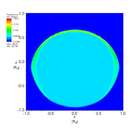
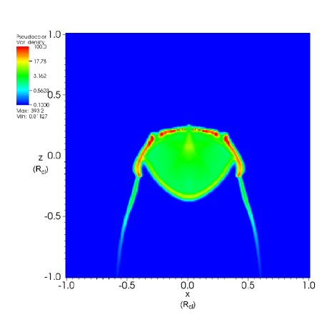
Figure 1: Slice of the logarithmic number density in the $y=0$ plane for the parallel shock model. The left panel shows the density distribution at 2.5 Myr (or just after t_cp) and the right panel at 9 Myr (or just after t_cc). The value of the number density is between 0.1 and 100 and the units of the axes are in $R_{cl}$.

3 Dynamical evolution

3.1 Parallel shock

The shock-cloud interaction for a parallel shock in 3D is nearly identical to the evolution studied in the 2D axisymmetric simulations of Paper I. It is useful to describe the dynamical evolution here again, not only to show the differences compared to the 2D results, but also because some of the dynamical characteristics are relevant for the perpendicular and oblique models.

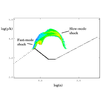
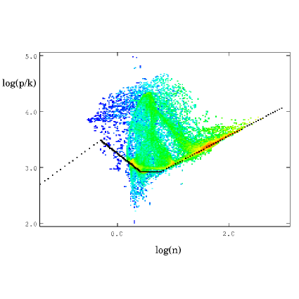
Figure 2: Distribution of the mass fraction in a phase diagram for the parallel shock model. The left panel shows the phase diagram at 2.5 Myr (or just after t_cp) and the right panel at 9 Myr (or just after t_cc). The values for the mass fraction range between 10^-6 and 10^-2. The black line represents the equilibrium curve.

Figure 1 shows results for the parallel case at two times. As the intercloud shock sweeps around the cloud (in a time of $t_{cp}=2R_{cl}/v_{ext}$), a shock is transmitted into the cloud and a bow-shock forms in front of the cloud. The transmitted fast-mode shock has a lower propagation speed than the intercloud shock, i.e. $v_{int}=v_{ext}/\chi^{1/2}$ where $\chi$ is the density ratio of cloud/intercloud gas. Therefore, a velocity shear layer forms at the cloud boundary. Because of this slip surface, a vortex ring develops and sweeps cloud material away from the cloud (see Fig. 1).

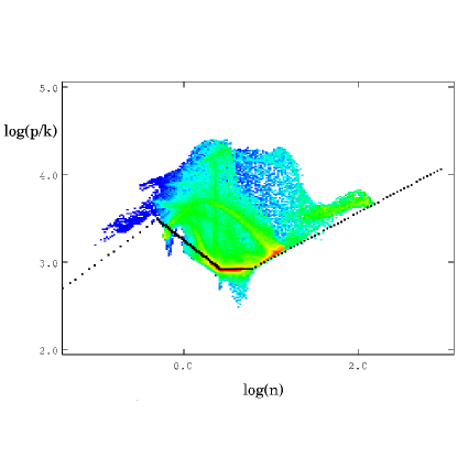
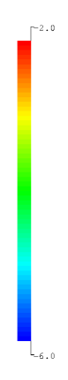
Figure 3: Similar to Fig. 2 but for the perpendicular shock model.

As the fast-mode shock moves through the cloud, it compresses and heats the initially thermally-stable warm gas so that it ends up being thermally unstable. Figure. 2 shows the distribution of mass in the $p-n$ phase space at two different times. The time scale for radiative cooling is shorter than the propagation time of the fast-mode shock through the cloud, given by the cloud-crushing time $t_{cc}=R_{cl}/v_{int}$. Thus, the gas loses a significant fraction of its internal energy during the compression. Furthermore, the magnetic pressure increases behind the fast-mode shock. Hence, the value of $\beta$ drops below unity inside the cloud. This provides the ideal conditions for the generation, by MHD waves, of dense clumps and cores (Falle & Hartquist, 2002; Van Loo, Falle, & Hartquist, 2006; Van Loo et al., 2008). Cold, dense clumps can also form due to small perturbations along the unstable part of the equilibrium curve (Inutsuka & Koyama, 2007). In our simulation we find a small fraction of cloud material on the thermally unstable part of the equilibrium curve after $\approx$ 6 Myr (or 0.7t_cc). Typical timescales for both processes are a few Myr. As the cloud flattens and fragments in about 1.5-2 t_cc (see Paper I), there is ample time for these processes to work. However, the numerical resolution of our simulations is insufficient to establish whether these processes are the dominant formation mechanisms of dense clumps and cores within clouds. As we cannot follow this formation process, we stop the simulation shortly after $t_{cc}$. This timescale was chosen because the re-expansion phase of the cloud then starts. Also, self-gravity which is not included in these simulations becomes globally important around this time and will affect the subsequent dynamical evolution.

The fast-mode shock is not the only shock to be transmitted into the cloud. A slow-mode shock is trailing the fast-mode shock. As it moves much more slowly than the fast-mode shock, it remains close to the boundary of the cloud. Behind the slow-mode shock, the magnetic pressure decreases and there is nothing that prevents the gas from compressing as it cools. Figure 2 clearly shows the rapid condensation due to the slow-mode shock. In a few Myr the gas behind the slow-mode shock cools to the thermally-stable cold phase. For the gas behind the fast-mode shock that is not processed by the slow-mode shock, this process occurs much more slowly.

Thus, a dense, cold layer quickly forms at the cloud boundary with the highest densities on the upstream parts of the cloud where the shock first hits the cloud (see Fig. 1). While the cooling behind the slow-mode shock is thermally unstable, the dense shell is subject to Kelvin-Helmholtz and Rayleigh-Taylor instabilities, even though the dynamical instabilities are mostly suppressed by the strong magnetic field (e.g. Chandrasekhar, 1961). Hence, the shell breaks up into dense fragments. The densest clumps have number densities of $\approx 10^{3}$  cm^-3 and are a few parsec in size. Note that we found roughly the same values for the higher resolution 2D simulation in Paper I. For lower resolution 2D simulations the densities are not so high. However, the clumps of the 2D simulations are essentially axisymmetric rings that break up into smaller, higher density clumps in the 3D simulations. These cold, dense clumps contain several hundreds of solar masses each and are gravitationally unstable. Thus, such clumps are likely precursors of massive stars.

3.2 Perpendicular shock

The dynamical evolution of cloud interacting with a perpendicular shock is in many ways similar to that of one interacting with a parallel shock. As the intercloud shock sweeps around the cloud, a transmitted fast-mode shock propagates through the cloud making the cloud material thermally unstable. Figure. 3 shows the distribution of mass in the $p-n$ phase space at two different times. The compression by a weak perpendicular shock is somewhat smaller than that by a parallel shock. The compression ratio changes from 2.70 for a parallel shock to 1.87 for a perpendicular shock. The gas behind the transmitted shock is therefore only marginally cooler and less dense.

However, contrary to what occurs in the parallel case, a slow-mode shock does not arise in the upstream parts of the cloud. This can be easily seen in Figs. 4 and 5 which show the logarithm of the density for the perpendicular case as a function of position for different slices and different times. Slow-mode waves, and therefore slow-mode shocks, do not propagate perpendicular to the magnetic field. However, as the intercloud shock sweeps across the cloud, a slow-mode shock does arise at the sides of the cloud. This slow-mode shock is not as strong as in the parallel case. Thus, it does not trigger a condensation near the boundary. Figure 3 shows that the transition from warm, rarefied gas to cold, dense gas is rather smooth with most of the gas near equilibrium. As discussed in Sect. 3.1, such a situation can initiate the formation of dense, cold clumps embedded in warm, rarefied gas (Inutsuka & Koyama, 2007).

The boundary layer in the perpendicular shock model is thus not as dense as in the parallel one. The maximum number density is an order of magnitude smaller $\approx 180$ cm^-3. Furthermore, the boundary layer is not subject to strong dynamical instabilities. While the boundary fragments into small, high-density clumps in the parallel model, it does not for the perpendicular model. Dynamical instabilities, notably the Kelvin-Helmholtz instability, take longer to develop due to a lower velocity shear and lower density, and are suppressed due to the strong magnetic field.

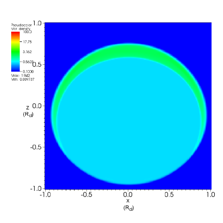
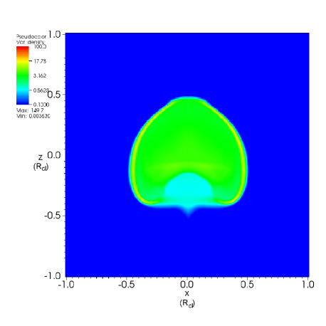
Figure 4: Similar to Fig. 1, but for the perpendicular shock model.

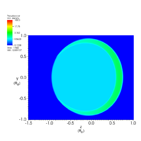
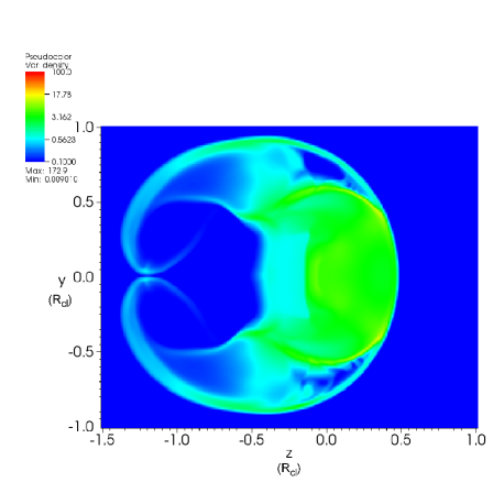
Figure 5: Similar to Fig. 4, but the slice is now in the $x=0$ plane.

As seen in Figs. 4 and 5, which are of the logarithmic density for different slices, instabilities are generated after some time, but only in a specific plane, i.e. in the $x=0$ plane. It is the only direction for which a shear layer forms in the perpendicular model. In contrast, in the parallel shock model the shear layer covers the entire cloud. The reason for this directional preference is found through the consideration of the vorticity equation, i.e.

$$\frac{\partial{\bf\omega}}{\partial t}=\nabla\times({\bf v}\times{\bf\omega})+\frac{1}{\rho^{2}}\nabla\rho\times\nabla(p+\frac{B^{2}}{2})-\frac{1}{\rho^{2}}\nabla\rho\times\left[({\bf B}.\nabla){\bf B}\right]$$

where ${\bf\omega}=\nabla\times{\bf v}$ is the vorticity. While the first term on the right hand side describes the stretching of vorticity, the second is the baroclinic term and accounts for the changes in the vorticity due to the intersection of density and thermal and magnetic pressure surfaces. The third term relates to the changes due to the interaction of the density gradient and magnetic tension forces. For flows with $\beta\gg 1$, the generation of vorticity is dominated by the thermal pressure contribution to the baroclinic term. This term does not introduce any directional preference. For the parallel shock model, the post-shock flow has a large $\beta$ and vorticity is generated all around the cloud. Figure 6 shows the downstream plasma beta as a function of the angle between the shock normal and the magnetic field. For flows with $\beta\leq 1$, the contribution of the magnetic field to the vorticity generation cannot be neglected. Magnetic tension forces then annul the generation of vorticity by the baroclinic term. It is thus clear that in regions where the magnetic field lines are being bent, no shear layer arises. For the perpendicular shock model, this is exactly what happens. The post-shock flow behind the intercloud shock drags the magnetic field with it along the $z$-direction. The field lines anchored in the cloud are bent and stretched in the $x,z$-plane near the cloud surface. Hence, less vorticity is generated in the $x,z$-plane and a shear layer is only present in the $x=0$ plane.

3.3 Oblique shock

The perpendicular and parallel shock models describe the extreme cases of the shock-cloud interaction. Therefore, we can expect that the dynamical evolution for oblique shocks lies in between those of the perpendicular and parallel models.

For an angle of 45^o between the shock normal and the magnetic field, the evolution of the cloud is similar to that of the perpendicular shock model. Although the transition of the gas from the warm to the cold phase is not as smooth as for the perpendicular shock model, it still progresses along the equilibrium curve. The maximum densities in the cloud are somewhat higher than for the perpendicular shock model. As for that model, the post-shock $\beta$ is $\approx 1$ (see Fig. 6). Thus, magnetic tension again prevents the formation of a shear layer surrounding the cloud. The preferential direction of shear layer is perpendicular to the initial magnetic field and the flow direction.

The 15^o oblique shock model does not resemble the geometrical evolution of the perpendicular shock-cloud interaction. Instead, the evolution better matches that of the parallel shock model as expected from the value of $\beta$ of the gas downstream the intercloud shock (Fig. 6). As the intercloud shock sweeps around the cloud, a shear layer forms all around the cloud. However, a higher level of shear is found in the plane perpendicular to the magnetic field and the flow direction. As for the parallel shock model, there is a rapid condensation behind the slow-mode shock and a dense boundary layer forms. This dense boundary layer, however, does not fragment due to instabilities as the small transverse component of the magnetic field has a stabilising effect. Although the geometrical features of the cloud resemble those of the parallel shock model, the cloud properties resemble those of the perpendicular model (see Sect. 4).

The shock-cloud interaction can thus be separated into two evolutionary tracks, i.e. one that is quasi-parallel and one that is quasi-perpendicular. From Fig. 6, we see that the transition is associated with the value of $\beta$ downstream of the intercloud shock. For parallel shocks the postshock flow has a $\beta>1$. Hence, the magnetic field is dynamically unimportant in the external gas which allows a vorticity layer to form around the cloud. For angles $>20^{o}$, the magnetic field is important and suppresses the generation of vorticity and shear layers.

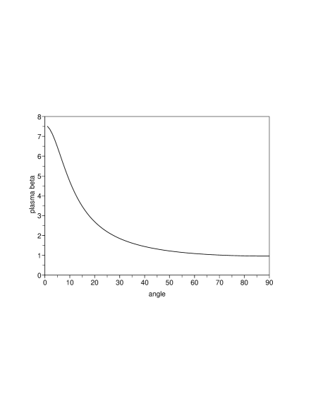
Figure 6: Plasma beta of the gas downstream the intercloud shock as a function of the angle between the magnetic field and shock normal.

4 Discussion of cloud properties

4.1 Size and density

In order to study the properties of the different shock-cloud interaction models, we use diagnostics similar to those used by previous authors, (e.g. Mac Low et al., 1994; Shin, Stone, & Snyder, 2008). Specifically, we use the density-weighted average of variables such as the plasma $\beta$ and the density using Eq. 1.

Furthermore, we define

$$a=\left[5\left(<x^{2}>-<x>^{2}\right)\right]^{1/2}.$$

along the $x$-axis, with similar expressions for analogous quantities defined along the $y$ and $z$-axes. This gives us the axes for an ellipsoid with a similar mass distribution as the cloud’s which are used to follow geometrical changes of the cloud. Figure 7 shows the temporal evolution of the volume of the cloud. The parallel shock compresses the cloud the most, while the perpendicular shock is the least compressive. At $t_{cc}$ the volume of the cloud is only a tenth of its original volume. The ram pressure exerted by the post-shock flow of the perpendicular shock is smaller than that for the parallel shock, as both the post-shock density and gas velocity (in the lab frame) are lower. (A parallel shock compresses gas more than a perpendicular shock with the same Mach number.) Furthermore, work needs to be done to compress the transverse magnetic field. Similarly, it is not surprising to find that the 45^∘ oblique shock squeezes the cloud faster than the perpendicular shock, but slower than the parallel shock. For smaller angles we expect the confinement of the cloud to converge to the parallel shock model. Indeed, the volume of the cloud in the 15^∘ oblique shock model changes as for the parallel shock model with only a small deviation at later times.

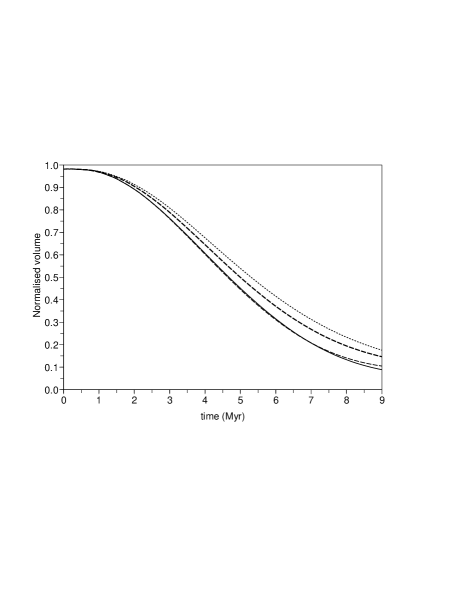
Figure 7: Mean cloud volume derived from the mass-weighted moments along the different axes for the parallel (solid), perpendicular (dotted) and oblique shock (thick dashed for 45^o and dashed for 15^o) cases. The volume is normalised to the initial cloud size.

Figure 7 seems to show a minimum in the volume near 9 Myr. From the 2D axisymmetric simulations, we know that a minimum arises as the fast-mode shock is reflected at the centre of the cloud at around $t_{cc}(\approx$ 8.3 Myr) and propagates back to the boundary. This shock reflection initiates a re-expansion phase in the direction perpendicular to the post-shock flow direction (see Mac Low et al., 1994, Paper I) Along the flow direction, the compression of the cloud continues and the cloud ends up as a thin disc after 1.5-2 $t_{cc}$. This means that the geometrical shape of the cloud resembles more closely an oblate spheroid than a sphere. The ellipticity of the cloud changes from 0 initially (i.e. a sphere) to roughly 0.5 at $t_{cc}$. As mentioned earlier, we do not follow this expansion phase and stop the simulation shortly after the cloud-crushing time $t_{cc}$.

Figure 8: rms number density of the cloud for the parallel (solid), perpendicular (dotted) and oblique shock (thick dashed for 45^o and thin dashed for 15^o) cases.

Figure 8 gives the evolution of the root-mean-square (rms) number density. Although the volumes of the cloud are only different by a factor of 2 as can be seen from Fig. 7, the rms density changes more significantly. At $t_{cc}$, the rms number density for the parallel model is $\approx 40$ cm^-3, while it is only 10 cm^-3 for the perpendicular model. This large variation is due to the large difference in the density of the boundary layer between the models (see Sect. 3). Only models with small angles between the shock normal and the magnetic field have mean densities similar to those of observed GMCs. Large angle models only reach mean densities similar to diffuse HI clouds. Such a dependence of the density structure on the magnetic field orientation is also observed by Heitsch, Stone, & Hartmann (2009).

Figure 9: Mass-weighted plasma beta of the cloud for the parallel (solid), perpendicular (dotted) and oblique shock model (thick dashed for 45^o and thin dashed for 15^o).

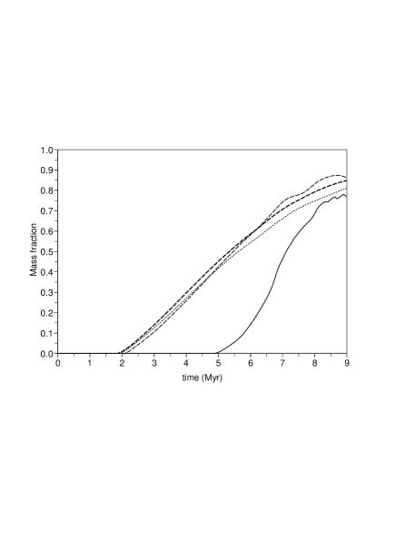
Figure 10: Mass fraction of the cloud with $\beta<0.1$ for the parallel (solid), perpendicular (dotted) and oblique shock model (thick dashed for 45^o and thin dashed for 15^o).

4.2 Thermal and magnetic pressure

Observations show that molecular clouds are magnetically dominated with plasma $\beta$ of the order 0.04 - 0.6 (Crutcher, Heiles, & Troland, 2003). Figure 9 shows the mass-weighed mean of $\beta$. This weighted mean value of $\beta$ for the parallel shock model does not lie within the observed range. During the early stages of the evolution the gas behind the slow-mode shock has a large thermal pressure, while the magnetic pressure is small. Hence, the plasma $\beta$ is large for the high-density gas in the boundary layer (which dominates the mean value of $\beta$), i.e. $\beta\approx 5$. After about 2.5 Myr, the weighted mean value of $\beta$ decreases as the thermally unstable gas behind the fast-mode shock becomes magnetically dominated. Although the weighted mean value of $\beta$ is now around unity, Fig. 10 shows that a significant mass fraction of the cloud has $\beta<0.1$. At $t_{cc}$, about 75% of the gas is significantly magnetically dominated.

The other models do produce a cloud with a weighted mean $\beta$ of the order of 0.4 (see Fig. 9). The main reason for this has to do with the role played by the transverse component of the magnetic field. While the thermal pressures behind the fast-mode and slow-mode shock are not as high as in the parallel shock model (i.e. the transition from the warm phase to the cold phase is smoother), the magnetic field is significantly compressed behind the fast-mode shock. The combined result of these effects produces a lower $\beta$ in both the boundary layer and within the cloud. Figure 10 indeed shows that magnetically-dominated gas appears much earlier for shock models with a transverse component to the magnetic field. After only 3 Myr, already 10% of the total mass in these models is magnetically dominated.

Our simulations show that, to produce clouds with magnetically-dominated high-density gas, the angle between the shock normal and the magnetic field must be small. While perpendicular shocks produce magnetically-dominated gas at low densities, high-density clumps with $\beta\gg 1$ arise in the parallel shock models.

4.3 Fragmentation

Our models show that large fractions of the cloud are magnetically dominated. This provides the ideal conditions for MHD waves to generate high-density clumps and cores within the cloud (Falle & Hartquist, 2002; Van Loo, Falle, & Hartquist, 2006; Van Loo et al., 2008). For shock models with a transverse component of the magnetic field, this process initiates earlier suggesting a higher degree of fragmentation. On top of that, another process is effective in these models. As the transition from the thermally-stable warm phase to the cold one follows the unstable part of the equilibrium curve, small perturbations can initiate the formation of dense, cold clumps embedded in warm, diffuse gas (Inutsuka & Koyama, 2007). Unfortunately, we cannot follow these clump and core formation processes as our resolution is insufficient.

While a low resolution is partly to blame for the low amount of fragmentation, the uniform initial conditions of the cloud also play an important role. In the colliding flow-driven models of Hennebelle et al. (2008) and Heitsch, Stone, & Hartmann (2009), the generation of cold dense cores and clumps relies on seeded perturbations in either the incoming flow or at the collision front. Without these perturbations, the collision region remains roughly uniform and fragmentation occurs on very long timescales. Therefore, it can be expected that the introduction of perturbations within the cloud and at the edge of the cloud would produce much more fragmentation.

Furthermore, our simulations do not include the effect of self-gravity. While self-gravity is dynamically unimportant for the global evolution of the cloud, i.e. the mass of the cloud is much smaller than its Jeans’ mass, its effect will become important locally. For example, the high-mass boundary layer clumps of the parallel shock model have masses that exceed their Jeans mass. We will investigate the effect of self-gravity on the cloud evolution in a later paper.

Figure 11: Mass fraction of cold (solid) and molecular (dashed) gas within the cloud for the parallel (thick) and perpendicular (thin) shock model. Molecular gas is assumed to be present when the thermal gas pressure is higher than 2500$k$ and the gas temperature lower than 100K.

4.4 Molecular clouds

Our simulations only describe the dynamical evolution of a cloud from warm atomic gas to cold atomic gas. Figure 11 shows the temporal evolution of the cold gas mass fraction for the parallel and perpendicular shock model. Cold gas arises earlier in the parallel shock model than in the perpendicular one, but after 9 Myr more than 50% of the initial cloud mass is in the thermally stable cold gas phase. Although we have not included a description of molecular cooling, nor do we follow the cloud chemistry, we can roughly estimate how much gas is converted from the cold atomic gas to molecular gas. Williams, Blitz, & Stark (1995) find that the average number density of H₂ in the CO clumps of the Rosette Molecular Cloud is $\approx 220~{}{\rm cm^{-3}}$. With typical excitation temperatures between 10 and 20 K, the thermal gas pressure of these clumps is roughly 2500k. Therefore, we assume that any gas parcel in the shocked cloud with a thermal pressure higher than 2500k and a temperature below 100K will become molecular given enough time (see below). Using this criterion, we find that the parallel shock model generates a molecular cloud as half of the cold gas becomes molecular (see Fig. 11). In the perpendicular cloud model only a small fraction of the cold atomic gas is converted into molecular gas. This suggests that the perpendicular shock model only produces a diffuse HI cloud.

The above result is only valid if the time scale for the formation of molecules is short and if the physical parameters of the formation process are met. Glover et al. (2009) use high-resolution 3D simulations of turbulent interstellar gas to follow the formation and destruction of molecular hydrogen and CO. They find that most CO forms within 2-3 Myr for dense, turbulent gas, while the formation of H₂ is even faster, i.e. within 1-2 Myr. Their results indicate that once large enough spatial and column densities are reached, the conversion from atomic to molecular gas is rapid. A good indictor for the formation of molecules is the visual extinction $A_{V}$, which can be expressed as (e.g. Chapuis & Corbel, 2004)

$$A_{V}=\frac{N_{H}}{1.80\times 10^{21}{\rm cm^{-2}}}.$$

For regions with $A_{V}\gtrsim 0.5$ and high local densities, we can then expect that molecules are present. Figure 12 shows that the visual extinction is already high early on in the parallel shock model. These regions also correspond to high-density regions, as can be seen in Fig. 1. This model thus most likely produces a molecular cloud. Also, note the similarity of the column density plot for the parallel shock model with the emission map of the W3 GMC (see Fig. 6 of Paper I). A more structured inner cloud can be expected with a non-uniform initial condition and a higher resolution.

While the 15^∘ oblique shock model also produces high column densities which coincide with high density regions, the perpendicular and the 45^∘ models do not. Models with large transverse components of the magnetic field produce diffuse HI clouds instead of molecular clouds. However, this conclusion only holds for our current simulations. A higher resolution and inclusion of small-scale perturbations potentially would produce higher density clumps for these models.

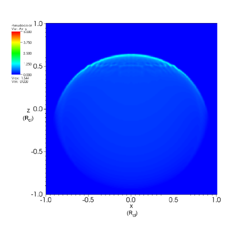
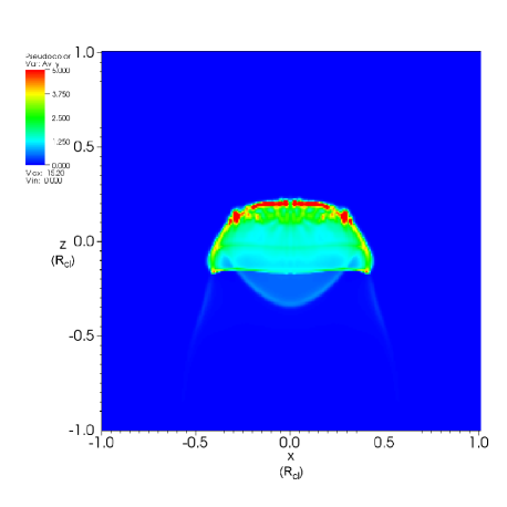
Figure 12: Visual extinction along the $y$-axis for a parallel shock interacting with a diffuse cloud. The left panel show the visual extinction at 2.5 Myr and the right panel at 9 Myr.

5 Summary

In this paper we have presented 3D simulations of the interaction of a weak, radiative shock with a magnetised, diffuse atomic cloud. The interaction of the shock induces the transition of the cloud from the thermally warm atomic phase to the cold one. By modelling the shock-cloud interaction in 3D, we are able to study the effect of different magnetic field orientations including parallel, oblique and perpendicular to the shock normal.

Contrary to the strong, adiabatic shock models of Shin, Stone, & Snyder (2008), we find that the structure of the shocked cloud differs significantly with the magnetic field orientation. The shock-cloud interaction can be separated into two distinct classes, i.e. a quasi-parallel one and a quasi-perpendicular one. In the quasi-parallel shock models high-density clumps are generated in the boundary layer surrounding the cloud. As the visual extinction of the gas is also high, the resulting cloud is most likely molecular. The quasi-perpendicular shock models, however, only produce low-density clouds resembling HI clouds. This result is similar to the one of Heitsch, Stone, & Hartmann (2009).

All our models show that the shocked cloud becomes magnetically dominated after a few Myr. Although this provides the ideal conditions for the formation of dense clumps and cores (Falle & Hartquist, 2002; Van Loo, Falle, & Hartquist, 2006; Van Loo et al., 2008), we do not see this happening in our simulations. This can be partly ascribed due to the assumption of an initially quiescent, uniform and spherical cloud. From the colliding flow-driven models we know that the inclusion of small-scale perturbations will generate a higher degree of structure. Increasing the resolution can have a similar effect (Yirak, Frank, & Cunningham, 2009). In a subsequent paper we will investigate the effect of small-scale perturbations and a higher resolution on the formation of clumps and cores.

References

- Ballesteros-Paredes & Hartmann (2007) Ballesteros-Paredes J., Hartmann L., 2007, RMxAA, 43, 123
- Begelman & McKee (1990) Begelman M. C., McKee C. F., 1990, ApJ, 358, 375
- Blitz & Stark (1986) Blitz L., Stark A. A., 1986, ApJ, 300, L89
- Chandrasekhar (1961) Chandrasekhar S., 1961, Hydrodynamic and hydromagnetic stability, Oxford University Press, London.
- Chapuis & Corbel (2004) Chapuis C., Corbel S., 2004, A&A, 414, 659
- Crutcher (1999) Crutcher R. M., 1999, ApJ, 520, 706
- Crutcher, Heiles, & Troland (2003) Crutcher R., Heiles C., Troland T., 2003, LNP, 614, 155
- Dedner et al. (2002) Dedner A., Kemm F., Kröner D., Munz C.-D., Schnitzer T., Wesenberg M., 2002, JCoPh, 175, 645
- Falle (1991) Falle S. A. E. G., 1991, MNRAS, 250, 581
- Falle & Hartquist (2002) Falle S. A. E. G., Hartquist T. W., 2002, MNRAS, 329, 195
- Field (1965) Field G. B., 1965, ApJ, 142, 531
- Field, Goldsmith, & Habing (1969) Field G. B., Goldsmith D. W., Habing H. J., 1969, ApJ, 155, L149
- Fragile et al. (2005) Fragile P. C., Anninos P., Gustafson K., Murray S. D., 2005, ApJ, 619, 327
- Glover et al. (2009) Glover S. C. O., Federrath C., Mac Low M. -M., Klessen R. S., 2009, arXiv, arXiv:0907.4081
- Gregori et al. (2000) Gregori G., Miniati F., Ryu D., Jones T. W., 2000, ApJ, 543, 775
- Heiles & Troland (2005) Heiles C., Troland T. H., 2005, ApJ, 624, 773
- Heitsch, Stone, & Hartmann (2009) Heitsch F., Stone J. M., Hartmann L. W., 2009, ApJ, 695, 248
- Hennebelle et al. (2008) Hennebelle P., Banerjee R., Vázquez-Semadeni E., Klessen R. S., Audit E., 2008, A&A, 486, L43
- Inoue & Inutsuka (2009) Inoue T., Inutsuka S.-i., 2009, ApJ, 704, 161
- Inutsuka & Koyama (2004) Inutsuka S., Koyama H., 2004, RMxAC, 22, 26
- Inutsuka & Koyama (2007) Inutsuka S., Koyama H., 2007, ASPC, 365, 162
- Klein & Woods (1998) Klein R. I., Woods D. T., 1998, ApJ, 497, 777
- Klessen, Krumholz, & Heitsch (2009) Klessen R. S., Krumholz M. R., Heitsch F., 2009, arXiv, arXiv:0906.4452
- Leão et al. (2009) Leão M. R. M., de Gouveia Dal Pino E. M., Falceta-Gonçalves D., Melioli C., Geraissate F. G., 2009, MNRAS, 394, 157
- Mac Low et al. (1994) Mac Low M.-M., McKee C. F., Klein R. I., Stone J. M., Norman M. L., 1994, ApJ, 433, 757
- Miniati et al. (1999) Miniati F., Ryu D., Ferrara A., Jones T. W., 1999, ApJ, 510, 726
- Moore et al. (2007) Moore T. J. T., Bretherton D. E., Fujiyoshi T., Ridge N. A., Allsopp J., Hoare M. G., Lumsden S. L., Richer J. S., 2007, MNRAS, 379, 663
- Nakamura et al. (2006) Nakamura F., McKee C. F., Klein R. I., Fisher R. T., 2006, ApJS, 164, 477
- Sánchez-Salcedo, Vázquez-Semadeni, & Gazol (2002) Sánchez-Salcedo F. J., Vázquez-Semadeni E., Gazol A., 2002, ApJ, 577, 768
- Shin, Stone, & Snyder (2008) Shin M.-S., Stone J. M., Snyder G. F., 2008, ApJ, 680, 336
- Stone & Norman (1992) Stone J. M., Norman M. L., 1992, ApJ, 390, L17
- Tachihara et al. (2002) Tachihara K., Onishi T., Mizuno A., Fukui Y., 2002, A&A, 385, 909
- Tokman (2006) Tokman, M., 2006, J.Comp.Phys., 213, 748
- Van Loo, Falle, & Hartquist (2006) Van Loo S., Falle S. A. E. G., Hartquist T. W., 2006, MNRAS, 370, 975
- Van Loo et al. (2007) Van Loo S., Falle S. A. E. G., Hartquist T. W., Moore T. J. T., 2007, A&A, 471, 213
- Van Loo et al. (2008) Van Loo S., Falle S. A. E. G., Hartquist T. W., Barker A. J., 2008, A&A, 484, 275
- Williams, Blitz, & Stark (1995) Williams J. P., Blitz L., Stark A. A., 1995, ApJ, 451, 252
- Wolfire et al. (1995) Wolfire M. G., McKee C. F., Hollenbach D., Tielens A. G. G. M., 1995, ApJ, 453, 673
- Yirak, Frank, & Cunningham (2009) Yirak K., Frank A., Cunningham A. J., 2009, arXiv, arXiv:0912.4777