Reliable source of conditional non-Gaussian states from single-mode thermal fields

Abstract

We address both theoretically and experimentally the generation of pulsed non-Gaussian states from classical Gaussian ones by means of conditional measurements. The setup relies on a beam splitter and a pair of linear photodetectors able to resolve up to tens of photons in the two outputs. We show the reliability of the setup and the good agreement with the theory for a single-mode thermal field entering the beam splitter and present a thorough characterization of the photon statistics of the conditional states.

I Introduction

The subtraction of photons from an optical field is of both fundamental and practical interest, because it is linked to the properties of the annihilation operator and plays a leading role in quantum information protocols involving non-Gaussian states generation, manipulation and distillation. In fact, the simplest way to generate a non-Gaussian optical state starting from a Gaussian one consists in subtracting photons from it. Photon subtraction can be implemented by inserting a beam splitter in the optical path of the original state, detecting the number of photons of the reflected portion and selecting the transmitted portion only if a certain condition on the number of detected photons is satisfied. The challenging part of this scheme is the use of detectors able to resolve the number of photons. As a matter of fact, if, on one hand, it is nowadays quite easy to detect a single photon (see, e.g., Ref. Par:JPB:09 and references therein), on the other hand, the limited availability of photon counters that can resolve higher numbers of photons has led to the quest for indirect ways to obtain such information rossi:PRA:04 ; zam:PRL:05 ; bri:JMO:09 .

It is worth mentioning that the subtraction of photons allows not only the generation of non-Gaussian states, but also the enhancement of the non-locality of bipartite states opa:PRA:00 ; coc:PRA:02 ; oli:PRA:03 ; inv:PRA:05 ; oli:LP:06 , or the generation of highly non-classical states wen:PRL:04 ; oli:JPB:05 useful for quantum information purposes cerf:05 . Nevertheless, non-Gaussianity is a necessary ingredient for continuous-variable entanglement distillation eisert:PRL:02 ; fiura:PRL:02 ; giedke:PRA:02 and different protocols relying on Gaussification of entangled non-Gaussian states browne:PRA:03 ; eisert:AOP:04 ; hage:NJP:07 or on de-Gaussification of entangled Gaussian states have been proposed taka:09 . In all these approaches an important role is played by photodetectors able to perform conditional measurements.

In this paper we report a thorough analysis of a setup based on hybrid photodetectors allowing the discrimination of the number of detected photons up to tens bon:ASL:09 ; bon:OL:09 . The aim of the paper is twofold: firstly we demonstrate the feasibility of our setup and, secondly, we investigate its reliability by characterizing the generated conditional states. The input Gaussian states we employ to achieve these goals are single-mode thermal fields. Thermal states are diagonal in the photon-number basis, thus, the knowledge of their photon statistics fully characterizes them and their conditional non-Gaussian counterparts, which are still diagonal. Thanks to this property, we can give a complete analytical description of the behavior of our setup, including the actual expressions of the conditional states, and we can verify the agreement between the theoretical expectations and the experimental results with very high accuracy and control. This is a fundamental test in view of the application of our setup to the generation of more sophisticated states by conditioning non-classical, multipartite and multimode ones twbrd .

Throughout the paper we investigate two possible scenarios. We refer to the first one as “conclusive photon subtraction” (CPS): a photon-number resolving detector is used to condition the signal and to conclude which is the effective number of subtracted photons. The second one is the “inconclusive photon subtraction” (IPS): an “on/off” Geiger-like detector, i.e., a detector only able to distinguish the presence from the absence of photons is employed, preventing us from inferring the actual number of subtracted photons.

The paper is structured as follows. Section II addresses the generation of conditional states by means of detectors with an effective photon-number resolving power. We discuss the model in the presence of non-unit quantum efficiency and give some analytical results. In Section III we briefly review the IPS process on thermal Gaussian fields; we also investigate the main properties of the generated conditional non-Gaussian states that will turn to be useful for the characterization of our setup. In Section IV we report the experimental demonstration of our scheme and thoroughly characterize the obtained conditional states. Section V closes the paper and draws some concluding remarks.

II Conditional non-Gaussian states from thermal fields via conditional measurements

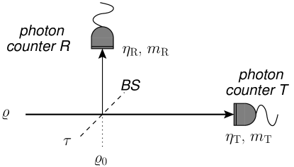
Figure 1: Scheme for the generation of conditional non-Gaussian states via photon subtraction. A thermal input state $\varrho$ is mixed with the vacuum state $\varrho_{0}=|0\rangle\langle 0|$ at a beam splitter (BS) with transmissivity $\tau$. Two photon counters (R, T) with quantum efficiency $\eta_{k}$, $k={\rm R},{\rm T}$, are used to generate and analyze conditional states. See text for details.

In Fig. 1 we depict the conditional photon-subtraction scheme based on a beam splitter (BS) and two photon-number resolving detectors. Although in our experimental realization we will consider only thermal states, for the sake of generality here we consider a diagonal state of the form $\varrho=\sum_{n}\varrho_{n}|n\rangle\langle n|$. After the evolution through the BS with transmissivity $\tau$, the initial two-mode state $R_{0}=\varrho\otimes|0\rangle\langle 0|$ is transformed into the state

$$R=\sum_{n=0}^{\infty}\varrho_{n}\sum_{k,l=0}^{n}A_{k}^{n}(\tau)A_{l}^{n}(\tau)|n-k\rangle\langle n-l|\otimes|k\rangle\langle l|,$$ (1)

where $A_{s}^{n}(\tau)=\sqrt{{n\choose s}\tau^{n-s}(1-\tau)^{s}}$. Then, the reflected part of the beam undergoes measurement. The positive-operator valued measure (POVM) describing a realistic photon counting device with quantum efficiency $\eta$ is given by DC:note

$$\Pi_{m}(\eta)=\sum_{s=m}^{\infty}B_{s,m}(\eta)|s\rangle\langle s|,$$ (2)

in which $B_{s,m}(\eta)={s\choose m}\eta^{m}(1-\eta)^{s-m}$. If the photon-counter in the reflected beam detects ${m_{\rm R}}$ photons, the conditional photon subtracted (CPS) state obtained in the transmitted beam is:

$$\varrho_{\rm CPS}({m_{\rm R}}) =\frac{1}{p_{\rm R}({m_{\rm R}})}{\rm Tr}_{\rm R}[R\,{\mathbbm{I}}\otimes\Pi_{m_{\rm R}}({\eta_{\rm R}})]$$

$$=\frac{1}{p_{\rm R}({m_{\rm R}})}\sum_{s={m_{\rm R}}}^{\infty}\sum_{n=0}^{\infty}B_{s,{m_{\rm R}}}({\eta_{\rm R}})$$

$$\hskip 42.67912pt\times\varrho_{s+n}\left[A_{s}^{s+n}(\tau)\right]^{2}|n\rangle\langle n|,$$ (3)

where $\eta_{k}$ is the quantum efficiency of the detector located in the reflected ($k={\rm R}$) and in the transmitted ($k={\rm T}$) beam paths, respectively. Note that the state in Eq. (II) is still diagonal. The overall probability $p_{\rm R}({m_{\rm R}})$ of measuring ${m_{\rm R}}$ in the reflected beam reads:

$$p_{\rm R}({m_{\rm R}})=\sum_{s={m_{\rm R}}}^{\infty}\sum_{n=0}^{\infty}B_{s,{m_{\rm R}}}({\eta_{\rm R}})\varrho_{n+s}\left[A_{s}^{n+s}(\tau)\right]^{2},$$ (4)

which represents the marginal distribution of the joint probability,

$$p_{\rm TR}({m_{\rm T}},{m_{\rm R}}) ={\rm Tr}[R\,\Pi_{m_{\rm T}}({\eta_{\rm T}})\otimes\Pi_{m_{\rm R}}({\eta_{\rm R}})]$$

$$=\sum_{t={m_{\rm T}}}^{\infty}\sum_{s={m_{\rm R}}}^{\infty}B_{s,{m_{\rm R}}}({\eta_{\rm R}})\,B_{t,{m_{\rm T}}}({\eta_{\rm T}})$$

$$\hskip 28.45274pt\times\left[A_{s}^{s+t}(\tau)\right]^{2}\,\varrho_{s+t},$$ (5)

that detectors T and R measure ${m_{\rm T}}$ and ${m_{\rm R}}$ photons, respectively. By taking $\varrho$ in a single-mode thermal state $\nu({N_{\rm th}})$,

$$\nu({N_{\rm th}}) =\sum_{n=0}^{\infty}\nu_{n}({N_{\rm th}})|n\rangle\langle n|,$$ (6)

$$\nu_{n}({N_{\rm th}}) =\frac{1}{1+{N_{\rm th}}}\left(\frac{{N_{\rm th}}}{1+{N_{\rm th}}}\right)^{n},$$ (7)

where ${N_{\rm th}}$ denotes the mean number of thermal photons, Eq. (5) reduces to

$$p_{\rm TR}({m_{\rm T}} ,{m_{\rm R}})={{m_{\rm T}}+{m_{\rm R}}\choose{m_{\rm R}}}\frac{{M_{\rm T}}^{{m_{\rm T}}}\,{M_{\rm R}}^{{m_{\rm R}}}}{(1+{M_{\rm T}}+{M_{\rm R}})^{{m_{\rm T}}+{m_{\rm R}}+1}},$$ (8)

${M_{\rm T}}=\tau\,{\eta_{\rm T}}\,{N_{\rm th}}$ and ${M_{\rm R}}=(1-\tau)\,{\eta_{\rm R}}\,{N_{\rm th}}$ being the mean numbers of detected photons of the transmitted and reflected beams, respectively.

Given ${m_{\rm R}}$ and $p_{\rm R}({m_{\rm R}})$, the conditional state $\varrho_{\rm CPS}$ in Eq. (II) can be obtained straightforwardly. From Eq. (II) we can then evaluate the Fano factor

$$F_{\rm CPS} =\frac{\sigma^{2}(M_{\rm CPS})}{M_{\rm CPS}},$$ (9)

which is the ratio between the variance $\sigma^{2}(M_{\rm CPS})$ and the mean number $M_{\rm CPS}$ of the photons detected in the CPS state. As we will see below, $F_{\rm T}\geq F_{\rm CPS}\geq 1$, where $F_{\rm T}=1+{M_{\rm T}}$ is the Fano factor of the single-mode thermal field of the (unconditional) transmitted beam. Note that $\varrho_{\rm CPS}$ is always super-Poissonian, which is consistent with the classical nature of the field.

To deeply characterize the output conditional state we evaluate its non-Gaussianity. Since the state has the form $\varrho_{\rm CPS}=\sum_{n}p_{n}|n\rangle\langle n|$, the non-Gaussianity (nonG) measure non:g can be written as:

$$\delta[\varrho_{\rm CPS}]=S[\nu(N_{\rm CPS})]+\sum_{n}p_{n}\log p_{n}$$ (10)

where $N_{\rm CPS}$ is the mean photon number of $\varrho_{\rm CPS}$, and $S[\nu(N)]=N\log(1+1/N)+\log(1+N)$ is the entropy of the thermal state $\nu(N)$.

However, due to the inefficient detection, we cannot reconstruct the actual photon number distribution $p_{n}$, but only the detected photon number distribution $q_{m_{\rm T}}=p_{\rm TR}({m_{\rm T}},\>{m_{\rm R}})$ given in Eq. (8), where ${m_{\rm R}}$ is the conditioning value, and ${m_{\rm T}}$ is the number of detected photons. Thus we can evaluate the quantity

$$\varepsilon[\varrho_{\rm CPS}]=S[\nu(M_{\rm CPS})]+\sum_{m_{\rm T}}q_{m_{\rm T}}\log q_{m_{\rm T}}\leq\delta[\varrho_{\rm CPS}].$$ (11)

The last inequality follows from the fact that the inefficient detection may be described by a Gaussian lossy channel that does not increase the non-Gaussianity, followed by an ideal (i.e., unit quantum efficiency) detection (see Appendix A for details). The quantity $\varepsilon[\varrho_{\rm CPS}]$, which can be easily evaluated from our experimental data, turns out to be a lower bound for the actual non-Gaussianity, that is, significant values of $\varepsilon[\varrho_{\rm CPS}]$ correspond to more markedly non-Gaussian states $\varrho_{\rm CPS}$.

III Inconclusive photon subtraction on thermal states

The conditional states introduced in the previous Section can be generated only if the detector in the reflected beam path is able to resolve the number of incoming photons. In this Section we consider a scenario in which the detector R (see Fig. 1) can only distinguish the presence from the absence of light (Geiger-like detector): we will refer to this measurement as inconclusive, as it does not resolve the number of the detected photons. When the detector clicks, an unknown number of photons is subtracted from $\varrho$ and we obtain the IPS state $\varrho_{\rm IPS}$. To characterize this class of conditional state, we use the phase-space description of the system evolution, that allows a simpler analysis with respect to that based on the photon number basis.

The phase-space description of the IPS operated on single-mode Gaussian states can be obtained by generalizing the analysis given in Ref. oli:JPB:05 . The Wigner function of the thermal state in Eq. (6) reads as follows (in Cartesian notation):

$$W_{\rm th}(\boldsymbol{X})=\frac{\exp\left(-\hbox{$\frac{1}{2}$}\boldsymbol{X}^{T}\boldsymbol{\sigma}_{\rm th}^{-1}\boldsymbol{X}\right)}{2\pi\sqrt{\hbox{Det}[\boldsymbol{\sigma}_{\rm th}]}},$$ (12)

where:

$$\boldsymbol{\sigma}_{\rm th}\equiv\boldsymbol{\sigma}_{\rm th}({N_{\rm th}})=\frac{1+2{N_{\rm th}}}{2}\,{\mathbbm{1}}$$ (13)

is the covariance matrix (CM), ${\mathbbm{1}}$ being the $2\times 2$ identity matrix. According to oli:JPB:05 , the action of the BS transforms the CM of the two-mode input state (thermal$+$vacuum)

$$\boldsymbol{\sigma}_{\rm in}=\left(\begin{array}[]{c|c}\boldsymbol{\sigma}_{\rm th}&{\boldsymbol{0}}\\ \hline\cr{\boldsymbol{0}}&\boldsymbol{\sigma}_{0}\end{array}\right)\,,$$ (14)

as follows FOP:napoli:05 :

$$\boldsymbol{\sigma}^{\prime}\equiv{\boldsymbol{S}}_{\rm BS}^{T}(\tau)\,\boldsymbol{\sigma}_{\rm in}\,{\boldsymbol{S}}_{\rm BS}(\tau)\equiv\left(\ \begin{array}[]{c|c}\boldsymbol{A}&\boldsymbol{C}\\ \hline\cr\boldsymbol{C}^{T}&\boldsymbol{B}\end{array}\right)\,,$$ (15)

where $\boldsymbol{A}$, $\boldsymbol{B}$, and $\boldsymbol{C}$ are $2\times 2$ matrices and

$$\boldsymbol{S}_{\rm BS}(\tau)=\left(\ \begin{array}[]{c|c}\sqrt{\tau}\,\mathbbm{1}&\sqrt{1-\tau}\,\mathbbm{1}\\ \hline\cr-\sqrt{1-\tau}\,\mathbbm{1}&\sqrt{\tau}\,\mathbbm{1}\end{array}\right)\,$$ (16)

is the symplectic transformation associated with the evolution operator $U_{\rm BS}$ of the BS.

The probability $p_{\rm on}=p_{\rm on}(r,\tau,{\eta_{\rm R}})$ that the on/off detector endowed with quantum efficiency ${\eta_{\rm R}}$ clicks is given by FOP:napoli:05 :

$$p_{\rm on} =1-p_{\rm off}(r,\tau,{\eta_{\rm R}})$$ (17)

$$=1-\left({\eta_{\rm R}}\sqrt{{\rm Det}[\boldsymbol{B}+\boldsymbol{\sigma}_{\rm M}]}\right)^{-1}$$ (18)

$$=\frac{{\eta_{\rm R}}(1-\tau){N_{\rm th}}}{1+{\eta_{\rm R}}(1-\tau){N_{\rm th}}}\,,$$ (19)

where $p_{\rm off}$ is the probability of a non-click event and

$$\boldsymbol{\sigma}_{\rm M}=\frac{2-{\eta_{\rm R}}}{2{\eta_{\rm R}}}\mathbbm{1}.$$ (20)

The Wigner function associated with the IPS state $\varrho_{\rm IPS}$ reads:

$$W_{\rm IPS}(\boldsymbol{X})=\frac{W_{a}(\boldsymbol{X})-p_{\rm off}\,W_{b}(\boldsymbol{X})}{p_{\rm on}},$$ (21)

where

$$W_{k}(\boldsymbol{X})=\frac{\exp\left(-\hbox{$\frac{1}{2}$}\boldsymbol{X}^{T}\boldsymbol{\Sigma}_{k}^{-1}\boldsymbol{X}\right)}{2\pi\sqrt{\hbox{Det}[\boldsymbol{\Sigma}_{k}]}},\quad(k=a,b)$$ (22)

$\boldsymbol{\Sigma}_{a}=\boldsymbol{A}$ and $\boldsymbol{\Sigma}_{b}=\boldsymbol{A}-\boldsymbol{C}(\boldsymbol{B}-\boldsymbol{\sigma}_{\rm M})\boldsymbol{C}^{T}$. Note that the IPS, being it the linear combination of two Gaussian functions, is no longer Gaussian: for this reason the IPS process is also referred to as a de-Gaussification process wen:PRL:04 . The Wigner functions in Eq. (22) are those of two thermal states $\nu(N_{k})$ with mean number of photons $N_{k}$ given by

$$N_{a}=\tau{N_{\rm th}},\quad N_{b}=\frac{\tau{N_{\rm th}}}{1+{\eta_{\rm R}}(1-\tau){N_{\rm th}}},$$ (23)

respectively; thus, the density matrix associated with (21) can be written as:

$$\varrho_{\rm IPS}=\frac{\nu(N_{a})-p_{\rm off}\,\nu(N_{b})}{p_{\rm on}},$$ (24)

and the corresponding conditional distribution of the detected photons is:

$$p_{T}({m_{\rm T}})=\frac{\nu_{{m_{\rm T}}}(M_{a})-p_{\rm off}\,\nu_{{m_{\rm T}}}(M_{b})}{p_{\rm on}},$$ (25)

where $M_{a}={\eta_{\rm T}}N_{a}$ and $M_{b}={\eta_{\rm T}}N_{b}$, being ${\eta_{\rm T}}$ the quantum efficiency of the photon-resolving detector of the IPS state, and the $\nu(N_{k})$ are given by Eq. (7).

Starting from the above results, we can give some further detail about the IPS thermal state in Eq. (24). The mean number of detected photons is

$$M_{\rm IPS}=\frac{M_{a}-p_{\rm off}\,M_{b}}{p_{\rm on}},$$ (26)

and the variance $\sigma^{2}(M_{\rm IPS})$ is:

$$\sigma^{2}(M_{\rm IPS})= \,\frac{M_{a}(1+M_{a})-p_{\rm off}\,M_{b}(1+M_{b})}{p_{\rm on}}$$

$$-\frac{p_{\rm off}(M_{a}-M_{b})^{2}}{p_{\rm on}^{2}}.$$ (27)

Moreover, as $M_{a}\geq M_{b}$, the Fano factor $F_{\rm IPS}$ is:

$$F_{\rm IPS} =\frac{\sigma^{2}(M_{\rm IPS})}{M_{\rm IPS}}$$ (28)

$$=1+M_{b}+2\frac{M_{a}(M_{a}-M_{b})}{M_{a}-p_{\rm off}\,M_{b}}-\frac{M_{a}-M_{b}}{1-p_{\rm off}}\geq 1,$$ (29)

in which the final inequality can be checked by substituting the actual expressions of $M_{a}$, $M_{b}$ and $p_{\rm off}$. The state is always super-Poissonian (also in this case, as one would expect, $F_{\rm T}\geq F_{\rm IPS}\geq 1$). As for the conditional states $\varrho_{\rm CPS}$, also in this case we can characterize the non-Gaussianity of the state $\varrho_{\rm IPS}$ from the experimental data by evaluating the quantity

$$\varepsilon[\varrho_{\rm IPS}]=S(\nu(M_{\rm IPS}))+\sum_{m_{\rm T}}q_{m_{\rm T}}\log q_{m_{\rm T}}\;,$$ (30)

which is still a lower bound for the non-Gaussianity measure, i.e. $\varepsilon[\varrho_{\rm IPS}]\leq\delta[\varrho_{\rm IPS}]$, as explained in the previous Section and in the Appendix A in more detail.

IV Reliable source of non-Gaussian states

IV.1 Experimental setup

We produced a single-mode pseudo-thermal state by inserting a rotating ground glass plate in the pathway of a coherent field, followed by a pin-hole to select a single coherence area in the far-field speckle pattern (see Fig. 2). As most detectors have the maximum quantum efficiency in the visible spectral range, we chose to exploit the second-harmonic linearly polarized pulses ($\lambda=523$ nm, 5.4 ps pulse duration) of a Nd:YLF mode-locked laser amplified at 500 Hz. The thermal light was split into two parts by a polarizing cube beam-splitter (PBS) whose transmissivity $\tau$ can be continuously varied by means of a half-wave plate ($\lambda$/2 in Fig. 2). We balanced the two exiting arms of the PBS to achieve $\tau\simeq 0.5$.

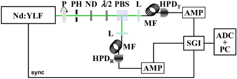
Figure 2: (Color online) Scheme of the experimental setup: P, rotating ground glass plate; PH, pin-hole; ND, continuously variable neutral density filter; $\lambda$/2, half-wave plate; PBS, polarizing cube beam-splitter; L, collective lens; MF, multi-mode fiber; HPD_R,T, hybrid photodetector; AMP, preamplifier plus amplifier; SGI, synchronous-gated integrator; ADC+PC, analog-to-digital converter.

The light exiting the PBS was focused in two multi-mode fibers and delivered to two hybrid photodetectors (HPD_R,T, mod. R10467U-40 Hamamatsu), endowed not only with a partial photon-resolving capability, but also with a linear response up to 100 incident photons. The outputs of the detectors were amplified (preamplifier A250 plus amplifier A275, Amptek), synchronously integrated (SGI, SR250, Stanford), digitized (ATMIO-16E-1, National Instruments) and processed offline. To analyze the outputs we model the detection process as a Bernoullian convolution and the overall amplification/conversion process through a very precise constant factor $\gamma$, which allows the shot-by-shot detector output to be converted into a number of detected photons JMO09 . The calibration procedure required performing a set of measurements of the light at different values of the overall detection efficiency of the apparatus, $\eta$, set by rotating a continuously variable neutral density filter wheel placed in front of the $\lambda$/2 plate. For each value of $\eta$, we recorded the data from $30\,000$ subsequent laser shots. For the results presented in the following we obtained the values $\gamma_{\rm R}=0.104$ V and $\gamma_{\rm T}=0.093$ V for the calibration of the detection chains in the reflected and transmitted arms of the beam splitter, respectively. These values of $\gamma_{\rm R,T}$ were used to convert the voltages into number of detected photons that were finally re-binned into unitary bins to obtain probability distributions. Once checked the reliability of the calibrations from the quality of these distributions, the voltage outputs of the HPD_R,T detectors were associated with numbers $m_{\rm R}$ and $m_{\rm T}$ in real time. The linearity of the detectors and the absence of significant dark counts make our system suitable for making experiments in both the CPS and IPS scenarios to produce conditional states. In the case of IPS, we only distinguish the HPD_R outputs giving $m_{\rm R}=0$ from those giving any $m_{\rm R}\geq 1$ to mimic the behavior of a Geiger-like detector.

IV.2 Conditional non-Gaussian states

The good photon-resolving capability of HPD detectors and their linearity make it possible to implement the CPS scheme described in Section II. Conditional measurements in the reflected beam irreversibly modify the states measured in the transmitted arm and in particular make them non-Gaussian.

To better understand the power and the limits of this kind of conditioning operation, we follow two different approaches: first of all we fix the energy ${N_{\rm th}}$ of the initial thermal field and characterize the CPS state as a function of the conditioning value ${m_{\rm R}}$. Secondly, we consider the properties of CPS states as a function of the mean incoming photons ${N_{\rm th}}$ for a particular choice of the number ${m_{\rm R}}$ of photons detected in the reflected arm. The final aim is the production of non-Gaussian states with well defined conditioning value.

We start by presenting the results obtained by choosing a set of measurements having $M_{\rm T}\approx 1.254$.

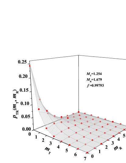
Figure 3: (Color online) Joint probability $p_{\rm TR}({m_{\rm T}},{m_{\rm R}})$ to measure ${m_{\rm R}}$ photons in the reflected beam and ${m_{\rm T}}$ photons in the transmitted one. The experimental data (red dots) are plotted together with the theoretical surface (gray mesh). The other involved experimental values are $M_{\rm R}=1.679$ and $M_{\rm T}=1.254$.

The joint probability $p_{\rm TR}({m_{\rm T}},{m_{\rm R}})$ of measuring ${m_{\rm R}}$ photons in the reflected arm and ${m_{\rm T}}$ photons in the transmitted one is plotted in Fig. 3 as dots together with the theoretical surface to which they perfectly superimpose. Of course, starting from the theoretical joint probability, we can calculate the expected photon-number distribution of the states obtained by performing different conditional measurements in the reflected arm [see Eq. (II)] and thus evaluate all the quantities necessary to characterize the CPS states.

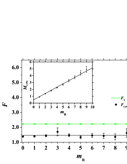
Figure 4: (Color online) Fano factors $F_{\rm CPS}$ of the conditional states: experiment (black dots) and theory (solid black line) as functions of the conditioning value ${m_{\rm R}}$. The green line corresponds to the Fano factor $F_{\rm T}=1+{M_{\rm T}}$ of the (unconditional) transmitted state. The inset refers to mean number of detected photons $M_{\rm CPS}$ of the CPS states as a function of the conditioning value ${m_{\rm R}}$: experimental data (dots) and theoretical curve (solid line). The values of the other involved parameters are $M_{\rm R}=1.679$ and $M_{\rm T}=1.254$.

In Fig. 4 we plot the behavior of the mean number of photons $M_{\rm CPS}$ of the conditional states and their Fano factors $F_{\rm CPS}$ as a function of the different conditioning values ${m_{\rm R}}$. We find that the Fano factor does not depend on the particular choice of the conditioning value ${m_{\rm R}}$, in agreement with the analytical result calculated from Eq. (8):

$$F_{\rm CPS}=\frac{1+M_{\rm T}+M_{\rm R}}{1+M_{\rm R}}\approx 1.468.$$ (31)

Note that the obtained value is definitely lower than that of the unconditional state, $F_{\rm T}\approx 2.225$.

The photon-number distributions of the conditional states look quite different from each other.

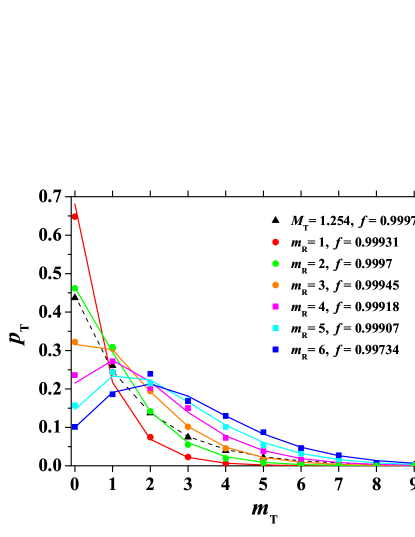
Figure 5: (Color online) Reconstructed photon-number distributions of the (unconditional) thermal state with mean number of photons $M_{\rm T}=1.254$ (black triangles) and of the conditional states for six different conditioning values ${m_{\rm R}}$ (colored dots and squares). The theoretical curves are plotted as lines according to the same choice of colors. The corresponding fidelity $f$ is also reported.

As it is shown in Fig. 5, the larger the conditioning value, the more different the statistics of the conditional state (colored symbols + lines) is from that of the incoming one (black triangles + dashed line). We note that, due to the limited number of recorded shots (only $30\,000$ laser-shots), the experimental points tend to deviate from the expected $p_{\mathrm{T}}$ distributions at increasing conditioning values. This behavior can be quantified by calculating the fidelity (see $f$ values reported in Fig. 5): $f=\sum^{\bar{m}}_{m=0}\sqrt{p^{\rm th}_{\rm T}(m)\,p_{\rm T}(m)}$, in which $p^{\rm th}_{\rm T}(m)$ and $p_{\rm T}(m)$ are the theoretical and experimental distributions, respectively, and the sum is extended up to the maximum detected photon number, $\bar{m}$, above which both $p^{\rm th}_{\rm T}(m)$ and $p_{\rm T}(m)$ become negligible. For all data displayed in Fig. 5 the fidelity is rather satisfactory.

Finally, the behavior of the lower bound for the nonG measure as a function of the conditioning value ${m_{\rm R}}$ (Fig.6) predicted by the theory (line) is well reproduced by the experimental data (dots).

Figure 6: Lower bound $\varepsilon[\varrho_{\rm CPS}]$ for the nonG measure $\delta[\varrho_{\rm CPS}]$ as a function of the conditioning value ${m_{\rm R}}$ for $M_{\rm T}=1.254$.

In particular, it is worth noting that the value of $\varepsilon[\varrho_{\rm CPS}]$ increases at increasing the conditioning value.

As an example of the second approach, we consider the CPS states obtained by choosing ${m_{\rm R}}=2$ as the conditioning value for different values of ${N_{\rm th}}$. In the inset of Fig. 7 the mean number of photons of the CPS states is plotted together with the mean number of photons of the initial states measured in the transmitted arm: it is interesting to notice that the values of $M_{\rm CPS}$ actually approach the conditioning value ${m_{\rm R}}=2$. Again, the experimental results (dots) are well superimposed to the theoretical curves, calculated starting from Eq. (II) with the measured mean values.

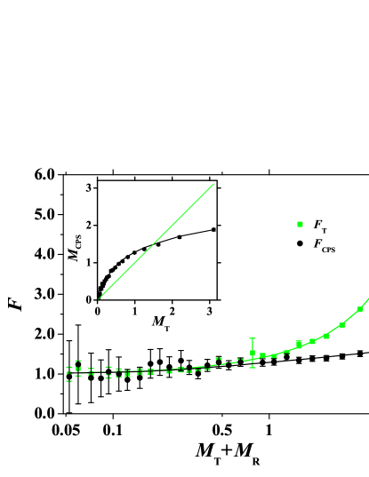
Figure 7: (Color online) Log-Linear plot of the Fano factors $F_{\rm CPS}$ of the CPS states (black dots) and of the unconditional states $F_{\rm T}$ (green squares) as functions of the total mean detected photons $M_{\rm T}+M_{\rm R}$ for conditioning ${m_{\rm R}}=2$. The solid lines refer to the corresponding theoretical curves. The inset shows the mean number of detected photons $M_{\rm CPS}$ of the CPS states as a function of the mean number of detected photons $M_{\rm T}$ of the unconditional states: experimental data (black dots) and theoretical curve (solid line). The green line refers to the mean photon number $M_{\rm T}$ of the unconditional states.

Figure 7 also shows the comparison between the Fano factor of the unconditional states $F_{\rm T}$ (green squares) and that of the CPS states $F_{\rm CPS}$ (black dots): as expected from theory the conditional states preserve the super-Poissonian nature of the incoming states, though with a smaller value of the Fano factor ($F_{\rm T}\geq F_{\rm CPS}\geq 1$).

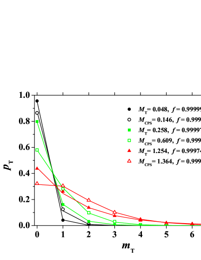
Figure 8: (Color online) Reconstructed photon-number distributions for three different examples (black, green, red) of unconditional states (full symbols) and for the corresponding CPS states (empty symbols) with ${m_{\rm R}}=2$. The theoretical curves are plotted as lines according to the same choice of colors. The corresponding fidelity $f$ is also reported.

In Fig. 8 we show three examples of conditional-state photon distributions for different values of the total incident intensity. For each example, we plot both the original thermal distribution (full symbols) and that of the conditional state (empty symbols). The agreement with the corresponding theoretical predictions (lines) is again testified by the high value of the fidelities.

Figure 9: Log-linear plot of the lower bound $\varepsilon[\varrho_{\rm CPS}]$ for the non-Gaussianity $\delta[\varrho_{\rm IPS}]$ as a function of the total mean detected photons $M_{\rm T}+M_{\rm R}$ and for ${m_{\rm R}}=2$: experimental data (dots) and theoretical curve (solid line).

We plot in Fig. 9 the lower bound for the non-Gaussianity $\varepsilon[\varrho_{\rm CPS}]$ as a function of the total mean detected photons (see Fig. 9) together with the expected theoretical results.

IV.3 IPS non-Gaussian states

Here we consider the scenario in which an on/off Geiger-like detector measures the reflected part of the input signal. In particular, as described in Section III, we are interested in studying the properties of the state produced in the transmitted arm of the PBS whenever the detector placed in the reflected arm clicks. To this aim, we performed a set of measurements by fixing the transmissivity of the PBS $\tau=0.5$ and changing the mean intensity of the light impinging on the PBS.

In the inset of Fig. 10 we plot the mean number of detected photons $M_{\rm IPS}$ of the IPS states as a function of the mean number of detected photons $M_{\rm T}$ of the unconditional thermal states (black dots) together with the theoretical prediction (solid line) according to Eq. (26). We note that the effect of the conditioning operation is to increase the mean value of the original state.

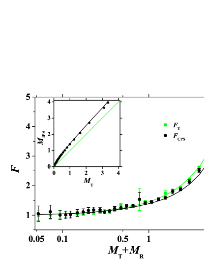
Figure 10: (Color online) Log-linear plot of the Fano factors $F_{\rm IPS}$ of the IPS states (black dots) and of the unconditional states (green squares) as functions of the total mean detected photons $M_{\rm T}+M_{\rm R}$. The solid lines refer to the corresponding theoretical curves. The inset shows the mean number of detected photons $M_{\rm IPS}$ of the IPS states as a function of the mean number of detected photons $M_{\rm T}$ of the unconditional states: experimental data (black dots) and theoretical curve (solid line). The green line refers to the mean photon number $M_{\rm T}$ of the unconditional states.

As described in Section III, another quantity to characterize the IPS state is the Fano factor $F_{\rm IPS}$: to better appreciate the difference between the unconditional states and the corresponding conditional ones, we plot in the same figure (see Fig. 10) the corresponding Fano factors as functions of the total mean detected photons (symbols). For each set of experimental results we also plot the theoretical behaviors (lines): analogously to the conditional case, we have $F_{\rm T}\geq F_{\rm IPS}\geq 1$.

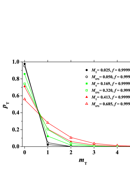
Figure 11: (Color online) Reconstructed photon-number distributions for three different examples (black, green, red) of unconditional states (full symbols) and for the corresponding IPS states (empty symbols). The theoretical curves are plotted as lines according to the same choice of colors. The fidelity $f$ is also reported.

In Fig. 11 we show the reconstruction of the detected photons distribution $p_{\rm T}({m_{\rm T}})$ of both the unconditional (full symbols) and the conditional states (empty symbols) for three different mean values (black, green, red) of the incident intensity. The agreement with the corresponding theoretical distributions (colored lines), calculated with the measured mean values, can be checked by evaluating the fidelity, as reported in Fig. 11.

Figure 12: Log-linear plot of the lower bound $\varepsilon[\varrho_{\rm IPS}]$ for the non-Gaussianity $\delta[\varrho_{\rm IPS}]$ as a function of the total mean detected photons $M_{\rm T}+M_{\rm R}$: experimental data (dots) and theoretical curve (line).

Finally, in Fig. 12 we plot the lower bound for the nonG measure $\varepsilon[\varrho_{\rm IPS}]$ as a function of the total mean detected photons. The correspondence between the experimental results (dots) and the theoretical prediction (line) is good. Note that $\varepsilon[\varrho_{\rm IPS}]$ increases as the mean number of detected photons increases: this allows the generation of highly populated non-Gaussian states.

V Concluding remarks

In this paper we have discussed in detail, both from a theoretical and an experimental point of view, a setup based on a single beam splitter and two photon-number resolving detectors to subtract photons from an incoming state and, thus, to generate non-Gaussian states starting from Gaussian ones. In order to show the reliability of our setup, we used (Gaussian) thermal states as inputs and completely characterized the conditional non-Gaussian outgoing states. In our analysis, we have adopted two possible detection schemes: the first one is based on the conclusive photon subtraction (CPS), whereas the second one on the inconclusive photon subtraction. In particular, we have demonstrated, as one may expect, that the non-Gaussianity of a state increases by increasing either the intensity of the input states or the conditioning value in the CPS scenario. This last condition requires photon-counting detectors endowed with a good linear response, such as those we used in our experiment.

The use of a class of diagonal states in the photon number basis (the thermal ones), allows us to obtain a high degree of control between the analytical theoretical expectations and the experiment, which is a relevant point in view of further investigations. In particular, we are planning to apply our schemes to more exotic classical states, such as the phase-averaged coherent states bon:ASL:09 . These are characterized by a non-Gaussian nature themselves, and, thus, the possibility to perform conditional, non-Gaussian measurements on them becomes particularly intriguing. Moreover, in this case analytical calculations may be carried out only to a certain extent: this is a clear example in which the reliability of the setup is a key point, as theoretical expectations are limited to numerical results.

Though we only focused on classical states, our experimental procedure opens the way to further developments toward the generation and engineering of more sophisticated quantum states by considering non-classical states as the inputs geno:PS:10 ; twbrd , which may be useful for quantum information protocols involving non-Gaussian states, such as entanglement distillation protocols browne:PRA:03 ; eisert:AOP:04 ; taka:09 .

Appendix A Experimental lower bound for the non-Gaussianity

For a single-mode state diagonal in the Fock basis, i.e., $\varrho=\sum_{n}p_{n}|n\rangle\langle n|$, the nonG measure non:g is given by

$$\delta[\varrho] =S[\nu(N)]-S(\varrho)=S[\nu(N)]+\sum_{n}p_{n}\log p_{n},$$ (32)

where $\nu(N)$ is a thermal state with mean photon number $N=\sum_{n}n\,p_{n}$. Being based on the knowledge of the actual photon distribution $p_{n}$, the calculation of $\delta[\varrho]$ requires measuring with an ideal (i.e., with unit quantum efficiency) photon-number resolving detector. In the presence of inefficient detection, one can only retrieve the detected photon number distribution $q_{m}={\rm Tr}[\varrho\Pi_{m}(\eta)]$, where $\Pi_{m}(\eta)$ is given in Eq. (2) and $\eta$ is the quantum efficiency. Nevertheless, in the following we will show that the quantity

$$\varepsilon[\varrho]=S[\nu(M)]+\sum_{m}q_{m}\log q_{m},$$ (33)

where $M=\sum_{m}m\,q_{m}=\eta N$, is a lower bound for the real non-Gaussianity $\delta[\varrho]$, i.e., $\varepsilon[\varrho]\leq\delta[\varrho]$. Note that since $\varepsilon[\varrho]$ depends only on $q_{m}$, it can be calculated starting from the experimental results.

The inefficient photodetection process can be described by mixing the quantum state $\varrho$ with the vacuum at a BS having transmissivity $\eta$ followed by perfect detection on the transmitted beam, thus obtaining

$$q_{m}={\rm Tr}[\mathcal{E}(\varrho)|m\rangle\langle m|],$$ (34)

where $\mathcal{E}(\varrho)={\rm Tr}_{2}[U_{BS}(\eta)\varrho\otimes|0\rangle\langle 0|U_{BS}^{\dagger}(\eta)]$ is the lossy Gaussian channel. Since $\varrho$ is diagonal in the Fock basis, $\mathcal{E}(\varrho)$ is still diagonal

$$\mathcal{E}(\varrho)=\sum_{n}p_{n}\mathcal{E}(|n\rangle\langle n|)=\sum_{m}q_{m}|m\rangle\langle m|,$$ (35)

in which $q_{m}=\sum_{n=m}^{\infty}p_{n}B_{n,m}(\eta)$. To obtain $\mathcal{E}(\varrho)$ we used $\mathcal{E}(|n\rangle\langle n|)=\sum_{l=0}^{n}B_{n,l}(\eta)|l\rangle\langle l|$, with $B_{n,l}(\eta)$ defined in Eq. (2). By using Eq. (32), we obtain

$$\delta[{\cal E}(\varrho)] =S[\nu(M)]+\sum_{n}q_{n}\log q_{n}=\varepsilon[\varrho].$$ (36)

As the nonG measure $\delta[\varrho]$ is non-increasing under Gaussian maps non:g , we finally get

$$\varepsilon[\varrho]=\delta[\mathcal{E}(\varrho)]\leq\delta[\varrho].$$ (37)

Summarizing, given a quantum state $\varrho$, diagonal in the Fock basis, we can measure the probability distribution of the detected phtotons $q_{m}$ and evaluate Eq. (33) as a lower bound for the actual non-Gaussianity $\delta[\varrho]$.

References

- (1) V. Parigi, A. Zavatta, and M. Bellini, “Implementation of single-photon creation and annihilation operators: experimental issues in their application to thermal states of light,” J. Phys. B: At. Mol. Opt. Phys. 42, 114005 (2009).
- (2) A. R. Rossi, S. Olivares, and M. G. A. Paris, “Photon statistics without counting photons,”, Phys. Rev. A 70, 055801 (2004).
- (3) G. Zambra, A. Andreoni, M. Bondani, M. Gramegna, M. Genovese, G. Brida, A. Rossi, and M. G. A. Paris, “Experimental reconstruction of photon statistics without photon counting,” Phys. Rev. Lett. 95, 063602 (2005).
- (4) G. Brida, M. Genovese, A. Meda, S. Olivares, M. G. A. Paris, and F. Piacentini, “Constrained MaxLik reconstruction of multimode photon distributions,” J. Mod. Opt. 56, 196 (2009).
- (5) T. Opatrný , G. Kurizki, and D.-G. Welsch, “Improvement on teleportation of continuous variables by photon subtraction via conditional measurement,” Phys. Rev. A 61, 032302 (2000).
- (6) P. T. Cochrane, T. C. Ralph, and G. J. Milburn, “Teleportation improvement by conditional measurements on the two-mode squeezed vacuum”, Phys. Rev. A 65, 062306 (2002).
- (7) S. Olivares, M. G. A. Paris, and R. Bonifacio, “Teleportation improvement by inconclusive photon subtraction,” Phys. Rev. A 67, 032314 (2003).
- (8) C. Invernizzi, S. Olivares, M. G. A. Paris, and K. Banaszek, “Effect of noise and enhancement of nonlocality in on/off photodetection,” Phys. Rev. A 72, 042105 (2005).
- (9) S. Olivares and M. G. A. Paris, “De-Gaussification by Inconclusive Photon Subtraction,” Laser Physics 16, 1533 (2006).
- (10) J. Wenger, R- Tualle-Brouri, and P. Grangier, “Non-Gaussian statistics from individual pulses of squeezed light,” Phys. Rev. Lett. 92, 153601 (2004).
- (11) S. Olivares and M. G. A. Paris, “Squeezed Fock state by inconclusive photon subtraction,” J. Opt. B: Quantum and Semiclass. Opt. 7, S616 (2005).
- (12) N. J. Cerf, O. Krüger, P. Navez, R. F. Werner, and M. M. Wolf, “Non-Gaussian cloning of quantum coherent states is optimal,” Phys. Rev. Lett. 95, 070501 (2005).
- (13) J. Eisert, S. Scheel, and M. B. Plenio, “On the impossibility of distilling Gaussian states with Gaussian operations,” Phys. Rev. Lett. 89, 137903 (2002).
- (14) J. Fiurášek, “Gaussian transformations and distillation of entangled Gaussian states,” Phys. Rev. Lett. 89, 137904 (2002).
- (15) G. Giedke and J. I. Cirac, “The characterization of Gaussian operations and distillation of Gaussian states,” Phys. Rev. A 66, 032316 (2002).
- (16) D. E. Browne, J. Eisert, S. Scheel and M. B. Plenio, “Driving non-Gaussian to Gaussian states with linear optics,” Phys. Rev. A 67, 062320 (2003).
- (17) J. Eisert, D. E. Browne, S. Scheel and M. B. Plenio, “Distillation of continuous-variable entanglement with optical means,” Annals of Physics (NY) 311, 431 (2004).
- (18) B. Hage, A. Franzen, J. DiGuglielmo, P. Marek, J. Fiurášek and R. Schnabel, “On the distillation and purification of phase-diffused squeezed states,” New J. Phys. 9, 227 (2007).
- (19) H. Takahashi, J. S. Neergaard-Nielsen, M. Takeuchi, M. Takeoka, K. Hayasaka, A. Furusawa, and M. Sasaki, “Non-Gaussian entanglement distillation for continuous variables,” eprint arXiv:0907.2159v1 [quant-ph].
- (20) M. Bondani, A. Allevi, and A. Andreoni, “Light statistics by non-calibrated linear photodetectors,” Adv. Sci. Lett. 2, 463 (2009).
- (21) M. Bondani, A. Allevi, and A. Andreoni, “Wigner function of pulsed fields by direct detection,” Opt. Letters 34, 1444 (2009).
- (22) A. Allevi, A. Andreoni, F. A. Beduini, M. Bondani, M. G. Genoni, S. Olivares, and M. G. A. Paris, unpublished.
- (23) The most general POVM describing a photon counting device also takes into account the presence of the dark counts; however, for the photodetectors we used in the experimental demonstration the number of the dark counts is negligible.
- (24) A. Ferraro, S. Olivares, and M. G. A. Paris, Gaussian States in Quantum Information (Bibliopolis, Napoli, 2005).
- (25) M. G. Genoni, M. G. A. Paris, and K. Banaszek, “Quantifying the non-Gaussian character of a quantum state by quantum relative entropy,” Phys. Rev. A 78, 060303(R), (2008).
- (26) V. C. Usenko, and M. G. A. Paris, “Losses and noise in quantum communication with photon-number entanlged states,” to appear in Phys. Lett. A (2010).
- (27) M. Bondani, A. Allevi, A. Agliati, and A. Andreoni, “Self-consistent characterization of light statistics,” J. Mod. Opt. 56, 226-231 (2009).
- (28) M. G. Genoni, F. A. Beduini, A. Allevi, M. Bondani, S. Olivares and M. G. A. Paris, “Non-Gaussian states by conditional measurements,” to appear in Physica Scripta (2010), e-print arXive:09095073v1 [quant-ph].