Determinant representation for some transition probabilities in the TASEP with second class particles

Abstract

Abstract: We study the transition probabilities for the totally asymmetric simple exclusion process (TASEP) on the infinite integer lattice with a finite, but arbitrary number of first and second class particles. Using the Bethe ansatz we present an explicit expression of these quantities in terms of the Bethe wave function. In a next step it is proved rigorously that this expression can be written in a compact determinantal form for the case where the order of the first and second class particles does not change in time. An independent geometrical approach provides insight into these results and enables us to generalize the determinantal solution to the multi-class TASEP.

I Introduction

In this paper we derive finite-time transition probabilities for the one-dimensional totally asymmetric simple exclusion process (TASEP) with several classes (species) of particles Ligg99 ; Schu01 . In the usual single-species TASEP in one dimension particles jump on the integer lattice ${\mathbb{Z}}$ independently after an exponentially distributed random time with parameter 1 to their right nearest neighbor site, provided that the target site is empty. Otherwise the jump attempt is rejected. This exclusion principle guarantees that each site is always occupied by at most one particle. An instantaneous configuration of this system with $N$ particles can therefore be represented by an ordered set of integer coordinates $\{\mathbf{x}\}=\{x_{1},\dots,x_{N}\}$ where $x_{i+1}>x_{i}$. An intuitive form to represent this lattice gas dynamics consists in writing allowed local transitions as

$$A0 \to 0A$$ (1)

where $A$ represents a particle and $0$ represents a vacant site. Mathematically, the dynamics of the TASEP can be defined through a master equation for the probability $P(\mathbf{x},t)$ to find a configuration $\mathbf{x}$ at time $t$. The master equation reads

$$\frac{d}{dt}P(\mathbf{x},t)=\sum_{\mathbf{x}^{\prime}\neq\mathbf{x}}\left[w_{\mathbf{x},\mathbf{x}^{\prime}}P(\mathbf{x}^{\prime},t)-w_{\mathbf{x}^{\prime},\mathbf{x}}P(\mathbf{x},t)\right],$$ (2)

where $w_{\mathbf{x}^{\prime},\mathbf{x}}$ is the transition rate (0 or 1 for the TASEP) to go from a configuration ${\bf x}$ to a configuration ${\bf x}^{{}^{\prime}}$. By integrating (2) one obtains the solution of the master equation for any given initial configuration $\mathbf{y}$, i.e., the conditional probability to find a particle configuration $\mathbf{x}$ at time $t$, given that the process started from configuration $\mathbf{y}$.

This process is a discretised version of the noisy Burgers equation Spoh91 ; burgers or, equivalently, the noisy Kardar-Parisi-Zhang equation Kard86 ; Sasa10 . On coarse-grained scale the Burgers equation exhibits shock solutions and it is of great interest to understand the microscopic structure of the shocks on the scale of the lattice. To this end, one introduces so-called second-class particles Ferr91 . We denote the first class particles by the symbol $A$ and the second class particles by the symbol $B$. According to the exclusion principle a lattice site can either be occupied by an $A$ particle, or a $B$ particle, or it can remain vacant (i.e. occupied by a hole, denoted as $0$). The exchange rules are

$$A0 \rightarrow 0A$$

$$B0 \rightarrow 0B$$ (3)

$$AB \rightarrow BA.$$

All processes occur with rate unity. Observe that from the perspective of the first-class particles the second-class particles are not distinguishable from holes. The stationary distribution of this two-component TASEP can be constructed using pair of independent product measures angel . It is well known that a single second-class particle in a system of first-class particles travels with the characteristic speed of the Burgers equation. Hence it can be used to define a microscopic position of the shock and to study its microscopic structure Ferr91 ; Ferr94 ; Derr97a ; Beli02 ; Kreb03 ; speer . It was also shown that a finite number of second class particles, in a uniform stationary background of first class particles, form a weak bound state Derr93c . The TASEP with second-class particles and more general two-component particle systems are also interesting from the point of view of non-equilibrium phase transitions godreche ; gms2003 ; blythe .

More generally, one may consider a hierarchical multi-class particle system where for a particle of class $k$ all particles of higher class behave like holes. This has interesting applications e.g. in the microscopic study of the so-called step initial condition where in an infinite system all sites $x\leq 0$ are occupied while the positive half lattice $x>0$ is vacant. This initial condition has been studied in great detail for the single-species TASEP, see e.g. the work by Johansson Joha00 for a seminal study of current fluctuations. Recently, interesting passing probabilities for the multi-class exclusion process have been obtained patricia . The stationary distribution of the multi-class TASEP has been constructed in jbmartin by extending the approach of angel . A matrix product formalism for the stationary measure of a multi-class TASEP was discussed in kirone .

A determinantal approach to solve for the dynamics of the single-species TASEP on the infinite lattice has been introduced in Schu97 . It is based on the explicit solution of the master equation for the conditional probability of finding the system in a certain configuration at time $t$ for a given initial configuration, using the technique of the Bethe Ansatz, originally employed for studying the relaxation spectrum of a periodic chain Gwa92 . Moreover, it was shown that the solution of master equation for $N$ particles on an infinite lattice can be written as the determinant of an $N\times N$ matrix. This determinantal form has allowed for a rederivation and extension of the work of Johansson on the step initial condition Naga04 ; Rako05 ; Prie08 and has inspired a substantial body of further work on other dynamical properties of the exclusion process, see e.g. Bran04 ; Sasa05 ; parallel ; Sasa07 ; Boro07 ; Boro08 ; Tracy1 ; Tracy2 . In the present work we obtain an exact solution of the master equation for a finite number of first class and second class particles on an infinite lattice with arbitrary initial condition. We use the nested Bethe ansatz schultz ; yang ; suth , thus generalizing the approach of Schu97 for the single-species case. In a recent study the technique of nested Bethe ansatz was used to investigate the spectral structure of the transition matrix for a multi-species exclusion process arita . In particular, the relaxation time-scale of the system was studied and it was shown that the dynamical exponent remains same as in the single-species case. In this paper, we use nested Bethe ansatz to solve the master equation of the two-species case. We obtain a compact determinantal representation of the solution for the case where first and second-class particles do not change their ordering. We also discuss the extension of our results to multi-species exclusion processes.

The paper is organized as follows. In Sec. II we show how the master equation can be solved exactly for the two-species case using the nested Bethe ansatz. In section III we give a formal proof of the determinantal representation for transition probabilities without interchange of particles. In section IV we present an alternative diagrammatic approach and discuss how using this approach the determinantal representation can be understood. We conclude this paper by discussing the possible generalization to multi-species systems in section V.

II Exact solution of the master equation using Bethe Ansatz

In this section we present an exact solution of the master equation for the TASEP with first and second class particles. To illustrate the approach we first consider the case of total particle number $N=2$. Each of these particles can be either of type $A$ or of type $B$. Therefore there are $4$ different particle sequences: $\{AA,AB,BA,BB\}$.

Let $x_{1},x_{2}$ with $x_{2}\geq x_{1}+1$ be the positions of the two particles at time $t$ and $y_{1},y_{2}$ be their initial positions with $y_{2}\geq y_{1}+1$. The quantity $P^{Q^{\prime}|Q}\left(x_{1},x_{2};t|y_{1},y_{2};0\right)$ denotes the probability to find the system in sequence $Q^{\prime}\in\{AA,AB,BA,BB\}$ with occupancies at $x_{1},x_{2}$ at time $t$, given that at $t=0$ the sequence was $Q\in\{AA,AB,BA,BB\}$ with occupied sites at $y_{1},y_{2}$. Note that if the initial sequence is $AA,BA$ or $BB$, then no interchange between $A$ and $B$ particles is possible as the system evolves in time. For these cases the sequence remains the same for all times and the particles execute usual TASEP dynamics with transition probabilities obtained in Schu97 . However, if the initial sequence is $AB$, then as a result of interchange between the $A$ and $B$ particles the sequence may change and the possible sequences at time $t$ are $AB,BA$.

In the absence of nearest neighbor pairs, i.e. for $x_{2}>x_{1}+1$, the master equation becomes

$$\frac{d}{dt}P^{Q^{\prime}|Q}(x_{1},x_{2};t|y_{1},y_{2};0)= P^{Q^{\prime}|Q}(x_{1}-1,x_{2};t|y_{1},y_{2};0)+P^{Q^{\prime}|Q}(x_{1},x_{2}-1;t|y_{1},y_{2};0)$$ (4)

$$-2P^{Q^{\prime}|Q}(x_{1},x_{2};t|y_{1},y_{2};0).$$

For $x_{2}=x_{1}+1$, the form of the equation is different depending on $Q$ and $Q^{\prime}$. For $Q\in\{AA,BA,BB\}$ we have $Q^{\prime}=Q$ and the equation takes the form

$$\frac{d}{dt}P^{Q|Q}(x_{1},x_{1}+1;t|y_{1},y_{2};0)=P^{Q|Q}(x_{1}-1,x_{1}+1;t|y_{1},y_{2};0)-P^{Q|Q}(x_{1},x_{1}+1;t|y_{1},y_{2};0).$$ (5)

For $Q=AB$ and $Q^{\prime}=AB$ we have

$$\frac{d}{dt}P^{AB|AB}(x_{1},x_{1}+1;t|y_{1},y_{2};0)=P^{AB|AB}(x_{1}-1,x_{1}+1;t|y_{1},y_{2};0)-2P^{AB|AB}(x_{1},x_{1}+1;t|y_{1},y_{2};0)$$ (6)

while for $Q=AB$ and $Q^{\prime}=BA$

$$\frac{d}{dt}P^{BA|AB}(x_{1},x_{1}+1;t|y_{1},y_{2};0)= P^{BA|AB}(x_{1}-1,x_{1}+1;t|y_{1},y_{2};0)+P^{AB|AB}(x_{1},x_{1}+1;t|y_{1},y_{2};0)$$ (7)

$$-P^{BA|AB}(x_{1},x_{1}+1;t|y_{1},y_{2};0).$$

To solve the above set of equations for a given initial sequence $Q$ and initial positions $\{y_{1},y_{2}\}$ we define

$$\left|P(t)\right\rangle=\left(\begin{array}[]{c}P^{AA|Q}(x_{1},x_{2};t|y_{1},y_{2};0)\\ P^{AB|Q}(x_{1},x_{2};t|y_{1},y_{2};0)\\ P^{BA|Q}(x_{1},x_{2};t|y_{1},y_{2};0)\\ P^{BB|Q}(x_{1},x_{2};t|y_{1},y_{2};0)\end{array}\right).$$ (8)

Notice that in order to keep the notation simple we do not mark the dependence of this vector on the initial sequence $Q$. Now we use Bethe Ansatz to write $\left|P(t)\right\rangle$ in the following form

$$\left|P(t)\right\rangle=\frac{1}{\left(2\pi\right)^{2}}\int_{0}^{2\pi}\int_{0}^{2\pi}dp_{1}dp_{2}e^{-\epsilon\left(p_{1},p_{2}\right)t}\left(e^{i\left(p_{1}x_{1}+p_{2}x_{2}\right)}+\Sigma\left(p_{1},p_{2}\right)e^{i\left(p_{2}x_{1}+p_{1}x_{2}\right)}\right)\left|P(0)\right\rangle$$ (9)

where

$$\left|P(0)\right\rangle=\left(\begin{array}[]{c}\delta_{AA,Q}\\ \delta_{AB,Q}\\ \delta_{BA,Q}\\ \delta_{BB,Q}\end{array}\right)e^{-i\left(p_{1}y_{1}+p_{2}y_{2}\right)}.$$ (10)

The elements of the $4\times 4$ matrix $\Sigma(p_{1},p_{2})$ and the quantity $\epsilon\left(p_{1},p_{2}\right)$ are yet undetermined functions of $p_{1}$ and $p_{2}$. Substituting this ansatz into (4) we find

$$\epsilon(p_{1},p_{2})=2-e^{-ip_{1}}-e^{-ip_{2}}$$ (11)

and to satisfy the boundary conditions for the nearest neighbor pairs resulting from Eqs (5), (6), (7), one needs

$$\Sigma(p_{1},p_{2})=\left(\begin{array}[]{cccc}-\frac{1-e^{ip_{2}}}{1-e^{ip_{1}}}&0&0&0\\ 0&-1&0&0\\ 0&-\frac{e^{ip_{1}}-e^{ip_{2}}}{1-e^{ip_{1}}}&-\frac{1-e^{ip_{2}}}{1-e^{ip_{1}}}&0\\ 0&0&0&-\frac{1-e^{ip_{2}}}{1-e^{ip_{1}}}\end{array}\right).$$ (12)

The complete solution can then be written in terms of the functions

$$F_{n}(x;t)=\frac{1}{2\pi}\int_{0}^{2\pi}dpe^{-t\left(1-e^{-ip}\right)}\frac{e^{ipx}}{\left(1-e^{i\left(p+i0\right)}\right)^{n}}.$$ (13)

introduced in Schu97 . From now on we will drop $t$ from the argument of the above function and write it simply as $F_{n}(x)$, for notational simplicity.

For the present case of two particles the values of $n$ that occur are $0,\pm 1$. For $Q=AA,BA,AB$ we have

$$P^{Q|Q}\left(x_{1},x_{2};t|y_{1},y_{2},0\right)=F_{0}(x_{1}-y_{1})F_{0}(x_{2}-y_{2})-F_{1}(x_{2}-y_{1})F_{-1}(x_{1}-y_{2})$$ (14)

and all other elements of $\left|P(t)\right\rangle$ with $Q^{\prime}\neq Q$ are zero. For $Q=AB$ we have

$$\left|P(t)\right\rangle=\left(\begin{array}[]{c}0\\ P^{AB|AB}\left(x_{1},x_{2};t|y_{1},y_{2},0\right)\\ P^{BA|AB}\left(x_{1},x_{2};t|y_{1},y_{2},0\right)\\ 0\end{array}\right)=\left(\begin{array}[]{c}0\\ F_{0}(x_{1}-y_{1})F_{0}(x_{2}-y_{2})-F_{0}(x_{2}-y_{1})F_{0}(x_{1}-y_{2})\\ F_{0}(x_{2}-y_{1})F_{0}(x_{1}-y_{2})-F_{1}(x_{2}-y_{1})F_{-1}(x_{1}-y_{2})\\ 0\end{array}\right)$$ (15)

The important point to note for $N\geq 3$ is that there are no new constraints from the boundary condition when more than two particles are on adjacent sites. This is expected from the integrability of the model Alca93 ; Popk02 , but we have also verified this explicitly in our calculation (see appendix). For $N=3$ there are $8$ possible sequences of $A$ and $B$, ordered in a vector $\left|P(t)\right\rangle$ according to the following formal tensor product:

$$\left(\begin{array}[]{c}A\\ B\end{array}\right)^{\otimes 3}=\left(\begin{array}[]{c}AAA\\ AAB\\ ABA\\ ABB\\ BAA\\ BAB\\ BBA\\ BBB\end{array}\right).$$ (16)

The Bethe Ansatz solution has the form

$$|P(t)\rangle=\frac{1}{(2\pi)^{3}}\int_{0}^{2\pi}dp_{1}dp_{2}dp_{3}e^{-\epsilon(p_{1},p_{2})t}\{e^{i(p_{1}x_{1}+p_{2}x_{2}+p_{3}x_{3})}$$

$$+\Sigma_{12}^{3}(p_{1},p_{2})e^{i(p_{2}x_{1}+p_{1}x_{2}+p_{3}x_{3})}+\Sigma_{23}^{3}(p_{2},p_{3})e^{i(p_{1}x_{1}+p_{3}x_{2}+p_{2}x_{3})}$$

$$+\Sigma_{23}^{3}(p_{1},p_{3})\Sigma_{12}^{3}(p_{1},p_{2})e^{i(p_{2}x_{1}+p_{3}x_{2}+p_{1}x_{3})}+\Sigma_{12}^{3}(p_{1},p_{3})\Sigma_{23}^{3}(p_{2},p_{3})e^{i(p_{3}x_{1}+p_{1}x_{2}+p_{2}x_{3})}$$

$$+\Sigma_{23}^{3}(p_{1},p_{2})\Sigma_{12}^{3}(p_{1},p_{3})\Sigma_{23}^{3}(p_{2},p_{3})e^{i(p_{3}x_{1}+p_{2}x_{2}+p_{1}x_{3})}\}|P(0)\rangle$$ (17)

where $\Sigma_{12}^{3}(p_{j},p_{k})=\Sigma(p_{j},p_{k})\otimes{\mathbb{I}}_{2}$ and $\Sigma_{23}^{3}(p_{j},p_{k})={\mathbb{I}}_{2}\otimes\Sigma(p_{j},p_{k})$. Here ${\mathbb{I}}_{2}$ is the $2\times 2$ unit matrix. Here the upper index 3 refers to the number of particles $N=3$. One crucial requirement for the integrability of the model is that these $\Sigma$-matrices must satisfy Yang-Baxter criterion (see appendix for details).

Using the definition in (13) the above solution can be written in terms of $F_{n}(x_{i}-y_{j})$ with $n=0,\pm 1,\pm 2$. For example, for the initial sequence $Q=AAB$ we find (with $\mathbf{x}=(x_{1},x_{2},x_{3}),\,\mathbf{y}=(y_{1},y_{2},y_{3})$)

$$P^{AAB|AAB}\left(\mathbf{x};t|\mathbf{y};0\right)=\left|\begin{array}[]{ccc}F_{0}(x_{1}-y_{1})&F_{-1}(x_{1}-y_{2})&F_{-1}(x_{1}-y_{3})\\ F_{1}(x_{2}-y_{1})&F_{0}(x_{2}-y_{2})&F_{0}(x_{2}-y_{3})\\ F_{1}(x_{3}-y_{1})&F_{0}(x_{3}-y_{2})&F_{0}(x_{3}-y_{3})\end{array}\right|$$ (18)

$$P^{ABA|AAB}\left(\mathbf{x};t|\mathbf{y};0\right)=F_{0}(x_{1}-y_{1})\left\{F_{0}(x_{2}-y_{3})F_{0}(x_{3}-y_{2})-F_{1}(x_{3}-y_{2})F_{-1}(x_{2}-y_{3})\right\}$$

$$+F_{-1}(x_{1}-y_{2})\left\{F_{2}(x_{3}-y_{1})F_{-1}(x_{2}-y_{3})-F_{0}(x_{2}-y_{3})F_{1}(x_{3}-y_{1})\right\}$$

$$+F_{0}(x_{2}-y_{1})\left\{F_{1}(x_{3}-y_{2})F_{-1}(x_{1}-y_{3})-F_{0}(x_{1}-y_{3})F_{0}(x_{3}-y_{2})\right\}$$

$$+F_{-1}(x_{2}-y_{2})\left\{F_{1}(x_{3}-y_{1})F_{0}(x_{1}-y_{3})-F_{2}(x_{3}-y_{1})F_{-1}(x_{1}-y_{3})\right\}$$ (19)

$$P^{BAA|AAB}\left(\mathbf{x};t|\mathbf{y};0\right)=F_{1}(x_{3}-y_{2})\left\{F_{1}(x_{2}-y_{1})F_{-2}(x_{1}-y_{3})-F_{0}(x_{2}-y_{1})F_{-1}(x_{1}-y_{3})\right\}$$

$$+F_{0}(x_{3}-y_{2})\left\{F_{0}(x_{1}-y_{3})F_{0}(x_{2}-y_{1})-F_{1}(x_{2}-y_{1})F_{-1}(x_{1}-y_{3})\right\}$$

$$+F_{2}(x_{3}-y_{1})\left\{F_{0}(x_{2}-y_{2})F_{-2}(x_{1}-y_{3})-F_{-1}(x_{2}-y_{2})F_{-1}(x_{1}-y_{3})\right\}$$

$$+F_{1}(x_{3}-y_{1})\left\{F_{-1}(x_{2}-y_{2})F_{0}(x_{1}-y_{3})-F_{0}(x_{2}-y_{2})F_{-1}(x_{1}-y_{3})\right\}$$ (20)

and all other components of $\left|P(t)\right\rangle$ are zero. Thus, starting from any given initial sequence $Q$, all components of $\left|P(t)\right\rangle$ can be determined.

Similarly, for $N=4$, the possible 16 sequences can be represented in the tensorial ordering $\left(\begin{array}[]{c}A\\ B\end{array}\right)^{\otimes 4}$. The Bethe Ansatz solution can be written down in terms of the matrices

$$\Sigma_{12}^{4}\left(p_{i},p_{j}\right) = \Sigma\left(p_{i},p_{j}\right)\otimes{\mathbb{I}}_{2}\otimes{\mathbb{I}}_{2}$$ (21)

$$\Sigma_{23}^{4}\left(p_{i},p_{j}\right) = {\mathbb{I}}_{2}\otimes\Sigma\left(p_{i},p_{j}\right)\otimes{\mathbb{I}}_{2}$$ (22)

$$\Sigma_{34}^{4}\left(p_{i},p_{j}\right) = {\mathbb{I}}_{2}\otimes{\mathbb{I}}_{2}\otimes\Sigma\left(p_{i},p_{j}\right)$$ (23)

and in this way one can construct $\left|P(t)\right\rangle$ for any value of $N$. The total of number of sequences is $2^{N}$ and these sequences are ordered as in

$$\left(\begin{array}[]{c}A\\ B\end{array}\right)^{\otimes N}$$

The $2^{N}$ dimensional $\Sigma$-matrices are constructed from the tensor product of $\Sigma(p_{i},p_{j})$ and ${\mathbb{I}}_{2}$ matrices:

$$\Sigma_{12}^{N}(p_{i},p_{j}) = \Sigma(p_{i},p_{j})\otimes{\mathbb{I}}_{2}\otimes{\mathbb{I}}_{2}\otimes.....\otimes{\mathbb{I}}_{2}$$ (24)

$$\Sigma_{23}^{N}(p_{i},p_{j}) = {\mathbb{I}}_{2}\otimes\Sigma(p_{i},p_{j})\otimes{\mathbb{I}}_{2}\otimes.....\otimes{\mathbb{I}}_{2}$$ (25)

etc. and in general

$$\Sigma_{k,k+1}^{N}(p_{i},p_{j}) = \left({\mathbb{I}}_{2}\right)^{\otimes k-1}\otimes\Sigma(p_{i},p_{j})\otimes\left({\mathbb{I}}_{2}\right)^{\otimes N-1-k}$$ (26)

The conditional probability $P^{Q^{\prime}|Q}\left(x_{1},x_{2},...,x_{N};t|y_{1},y_{2},...,y_{N};0\right)$ has the Bethe ansatz form

$$\left|P(t)\right\rangle=\frac{1}{(2\pi)^{N}}\int_{0}^{2\pi}dp_{1}dp_{2}...dp_{N}\sum_{\{Q\}}{\cal P}(Q_{1}Q_{2}...Q_{N})e^{i\left(p_{Q_{1}}x_{1}+p_{Q_{2}}x_{2}+...+p_{Q_{N}}x_{N}\right)}\left|P(0)\right\rangle.$$ (27)

In this Bethe representation $\{Q_{1}Q_{2}...Q_{N}\}$ is one particular permutation of $\{12...N\}$ and ${\cal P}(Q_{1}Q_{2}...Q_{N})$ is constructed from the product of $\Sigma_{i,i+1}^{N}\left(p_{k},p_{j}\right)$ matrices given by Eq. (26). This product corresponds to the series of elementary permutations performed on the momenta $\{p_{1},p_{2},...,p_{N}\}$ to arrange them in the order $\{p_{Q_{1}},p_{Q_{2}},...,p_{Q_{N}}\}$. The summation is over all possible $N!$ permutations. One can show by adapting the techniques of Popk02 that Eq. (27) solves the $N$-particle master equation for the TASEP with second class particles.

Notice that the matrix $\Sigma$ in Eq. (12) may be decomposed as $\Sigma=D+A$ where $D$ is the diagonal part and $A$ the off-diagonal part which arises from the interchange $AB\to BA$ of the two species of particles. Correspondingly the product ${\cal P}(Q_{1}Q_{2}...Q_{N})$ can be expanded in terms containing an increasing number of $A$ matrices which represent the number of interchanges in the final configuration. The purely diagonal part in this expansion corresponds to configurations in which the original order of first and second-class particles has not changed. We investigate these realizations of the stochastic dynamics in more detail in the following section.

III Theorem for no interchange

In the previous section we have shown that using Bethe Ansatz it is possible to solve the master equation for any number of particles with any sequence. The Bethe Ansatz form of the solution for $N$ particles has, in general, $N!$ number of terms. In the single-species TASEP case, it was shown in Schu97 that the solution of the master equation can be written as a determinant of a matrix $F$ whose elements are $F_{ij}=F_{i-j}(x_{i}-y_{j})$ with $F_{i-j}(x_{i}-y_{j})$ defined according to (13). In this section we show that there is compact determinant representation of the transition probability for the case where no interchange between $A$ and $B$ particles takes place, i.e., where the sequence at time $t$ is the same as the initial sequence at time $t=0$. We state the main result:

Theorem for no interchange: Consider a system of $N$ particles, each of species $A$ or $B$, starting with an initial sequence $Q$ at time $t=0$ taken from the tensorial ordering

$$\left(\begin{array}[]{c}A\\ B\end{array}\right)^{\otimes N}.$$

The probability $P^{Q|Q}\left(x_{1},x_{2},...,x_{N};t|y_{1},y_{2},...,y_{N};0\right)$ where the initial and final sequence remains the same can be written as the determinant of the $N\times N$ matrix $G$, where

$$G_{ij}=F_{n(i,j)}\left(x_{i}-y_{j}\right)$$ (28)

with matrix elements $F_{n}$ defined in (13) and $n(i,j)=sgn(i-j)\left(|i-j|-n_{AB}\right)$ with $n_{AB}$ being the number of $AB$ pairs occurring between the $i$-th and $j$-th particle of the sequence $Q$.

Remark: To illustrate this result, to be proved rigorously below, consider e.g. the sequence $AABABBAB...$. Here $n(1,3)=-1$, $n(1,7)=-4$, $n(8,4)=2$, $n(3,3)=0$, and so on. Note that if a sequence $Q$ has no $AB$ pair, $n_{AB}=0\,\forall\,i,j$ and the matrix $G$ becomes identical to the matrix found in Schu97 . This is expected since the system behaves in this case like a single-species TASEP.

Proof: We have to show first that $\det G$ satisfies the master equation. In the absence of any nearest neighbor pair, the master equation is

$$\frac{d}{dt}P^{Q|Q}\left(\mathbf{x};t|\mathbf{y};0\right)=\sum_{i=1}^{N}P^{Q|Q}\left(x_{1},x_{2},...,x_{i-1},x_{i}-1,x_{i+1},...,x_{N};t|\mathbf{y};0\right)$$

$$-NP^{Q|Q}\left(\mathbf{x};t|\bf y;0\right).$$ (29)

Since all the elements of the matrix $G$ contain the factor $e^{-t}$, one can write $G=e^{-t}\tilde{G}$ which gives

$$\frac{d}{dt}\det G=e^{-Nt}\frac{d}{dt}\det\tilde{G}-N\det G.$$ (30)

Now the time-derivative in the first term on right-hand side can be written as

$$\frac{d}{dt}\left|\begin{array}[]{cccc}\tilde{G}_{11}&\tilde{G}_{12}&...&\tilde{G}_{1N}\\ \tilde{G}_{21}&\tilde{G}_{22}&...&\tilde{G}_{2N}\\ ...&...&...&...\\ \tilde{G}_{N1}&\tilde{G}_{N2}&...&\tilde{G}_{NN}\end{array}\right|=\left|\begin{array}[]{cccc}{\dot{\tilde{G}}}_{11}&{\dot{\tilde{G}}}_{12}&...&{\dot{\tilde{G}}}_{1N}\\ \tilde{G}_{21}&\tilde{G}_{22}&...&\tilde{G}_{2N}\\ ...&...&...&...\\ \tilde{G}_{N1}&\tilde{G}_{N2}&...&\tilde{G}_{NN}\end{array}\right|$$ (39)

$$+\left|\begin{array}[]{cccc}\tilde{G}_{11}&\tilde{G}_{12}&...&\tilde{G}_{1N}\\ {\dot{\tilde{G}}}_{21}&{\dot{\tilde{G}}}_{22}&...&{\dot{\tilde{G}}}_{2N}\\ ...&...&...&...\\ \tilde{G}_{N1}&\tilde{G}_{N2}&...&\tilde{G}_{NN}\end{array}\right|+...+\left|\begin{array}[]{cccc}\tilde{G}_{11}&\tilde{G}_{12}&...&\tilde{G}_{1N}\\ \tilde{G}_{21}&\tilde{G}_{22}&...&\tilde{G}_{2N}\\ ...&...&...&...\\ {\dot{\tilde{G}}}_{N1}&{\dot{\tilde{G}}}_{N2}&...&{\dot{\tilde{G}}}_{NN}\end{array}\right|$$ (48)

The $i$-th row of $\tilde{G}$ is $\left\{{\tilde{G_{i1}}},{\tilde{G_{i2}}},...{\tilde{G_{iN}}}\right\}=\left\{{\tilde{F}_{n(i,1)}}(x_{i}-y_{1}),{\tilde{F}_{n(i,2)}}(x_{i}-y_{2}),...,{\tilde{F}_{n(i,N)}}(x_{i}-y_{N})\right\}$ where we have used the notation $F=e^{-t}\tilde{F}$.

To find the time-derivative of these elements of the $i$-th row we use the identity ${\dot{F}}_{n}(x)=-F_{n}(x)+F_{n-1}(x-1)$ from which it follows that ${\dot{\tilde{F}}}_{n}(x)={\tilde{F}}_{n}(x-1)$. Therefore, taking the time derivative generates the row $\left\{{\tilde{F}_{n(i,1)}}(x_{i}-1-y_{1}),{\tilde{F}_{n(i,2)}}(x_{i}-1-y_{2}),...,{\tilde{F}_{n(i,N)}}(x_{i}-1-y_{N})\right\}$. Thus each term on the r.h.s. of (48) contributes to one term in the summation in Eq. (29). From Eq. (30) it follows therefore that $\det G$ satisfies Eq. (29).

Now consider the case when one nearest neighbor pair is present: $x_{j}=x_{j-1}+1$. If the $(j-1)$-th particles is $A$ and the $j$-th one is $B$, then the master equation becomes

$$\frac{d}{dt}P^{Q|Q}\left(\mathbf{x};t|\mathbf{y};0\right)=\sum_{i\neq j}P^{Q|Q}\left(x_{1},x_{2},...,x_{i-1},x_{i}-1,x_{i+1},...,x_{N};t|\mathbf{y};0\right)$$

$$-NP^{Q|Q}\left(x_{1},x_{2},...,x_{N};t|y_{1},\mathbf{y};0\right).$$ (49)

which gives rise to the boundary condition

$$P^{Q|Q}\left(x_{1},x_{2},...,x_{j-1},x_{j-1},x_{j+1},...,x_{N};t|\mathbf{y};0\right)=0$$ (50)

to be satisfied at all times. Since there is an $AB$ pair at $(j-1),j$, from the definition of $n(i,j)$ it follows that $n(i,j-1)=n(i,j)$ $\forall i$. Hence in the determinantal representation of $P^{Q|Q}\left(x_{1},x_{2},...,x_{j-1},x_{j-1},x_{j+1},...,x_{N};t|\mathbf{y};0\right)$ the $(j-1)$-th and $j$-th row becomes identical and the determinant vanishes. If the $(j-1)$-th particle is $B$ and the $j$-th one is $A$ then the boundary condition is

$$P^{Q|Q}\left(x_{1},x_{2},...,x_{j-1},x_{j-1},x_{j+1},...,x_{N};t|\mathbf{y};0\right)=$$ (51)

$$P^{Q|Q}\left(x_{1},x_{2},...,x_{j-1},x_{j-1}+1,x_{j+1},...,x_{N};t|\mathbf{y};0\right)$$

which becomes

$$\left|\begin{array}[]{ccc}...&...&...\\ F_{n(j-1,1)}(x_{j-1}-y_{1})&F_{n(j-1,2)}(x_{j-1}-y_{2})&...\\ F_{n(j-1,1)+1}(x_{j-1}-y_{1})&F_{n(j-1,2)+1}(x_{j-1}-y_{2})&...\\ ...&...&...\end{array}\right|=$$ (56)

$$\left|\begin{array}[]{ccc}...&...&...\\ F_{n(j-1,1)}(x_{j-1}-y_{1})&F_{n(j-1,2)}(x_{j-1}-y_{2})&...\\ F_{n(j-1,1)+1}(x_{j-1}+1-y_{1})&F_{n(j-1,2)+1}(x_{j-1}+1-y_{2})&...\\ ...&...&...\end{array}\right|$$ (61)

which can be proved using $F_{n(j-1,i)+1}(x_{j-1}+1-y_{i})=F_{n(j-1,i)+1}(x_{j-1}-y_{i})-F_{n(j-1,i)}(x_{j-1}-y_{i})$. If $(j-1)$-th and $j$-th particles are $AA$ or $BB$, then the corresponding boundary condition becomes

$$P^{Q|Q}\left(x_{1},x_{2},...,x_{j-1},x_{j-1},x_{j+1},...,x_{N};t|\mathbf{y};0\right)=$$ (62)

$$P^{Q|Q}\left(x_{1},x_{2},...,x_{j-1},x_{j-1}+1,x_{j+1},...,x_{N};t|\mathbf{y};0\right)$$

which is easily shown to be satisfied using the identity $F_{n}(x+1)=F_{n}(x)-F_{n-1}(x)$.

Finally we have to show that $\det G$ satisfies the correct initial condition. To this end note first the identity $F_{n}(x;t=0)=\delta_{x,0}$ which follows from the definition of $F_{n}(x;t)$ in (13). This means that for $x_{1}>y_{1}$ all the elements of the first column must vanish: $G_{i1}=0$ for $t=0$ which yields $detG=0$. For $x_{1}=y_{1}$ one has $G_{11}=1$ and $G_{i1}=0$ $\forall i\neq 1$, since $x_{i}>y_{1}$ for $i>1$. Then $\det G$ becomes equal to $\delta_{x_{1},y_{1}}\det G^{(1)}$ where the matrix $G^{(1)}$ is obtained from $G$ after omitting the first row and the first column. Next, we assume $x_{2}>y_{2}$ and using the above identity, we have $G^{(1)}_{i1}=0$ $\forall i$ and for $x_{2}=y_{2}$ $G^{(1)}_{i1}=\delta_{i,1}$. It follows therefore that $\det G=\delta_{x_{1},y_{1}}\delta_{x_{2},y_{2}}\det G^{(2)}$, with $G^{(2)}$ being an $(N-2)$ dimensional matrix which results from omitting first two rows and columns of $G$. Repeating the above procedure $N$ times, one finds

$$\det G|_{t=0}=\prod_{i=1}^{N}\delta_{x_{i},y_{i}}.$$ (63)

This completes the proof of the theorem stated above.

IV Geometrical treatment of the Bethe Ansatz solution

In this section, we use the geometrical interpretation of the Bethe Ansatz introduced in dia1 ; dia2 to analyze the entangled systems of allowed and forbidden trajectories of different species of particles. This approach serves as a heuristic alternative to the explicit rigorous solution of the master equation.

To illustrate this approach let us first consider the single-species TASEP with $N=2$. The solution of the master equation in this case is Schu97

$$F_{0}(x_{1}-y_{1})F_{0}(x_{2}-y_{2})-F_{1}(x_{2}-y_{1})F_{-1}(x_{1}-y_{2}).$$ (64)

Instead of the TASEP let us now consider two vicious random walkers (VRW) where two particles perform biased random walks on a lattice and if they jump on each other, they annihilate. It is easy to verify that the solution of master equation in this case is

$$F_{0}(x_{1}-y_{1})F_{0}(x_{2}-y_{2})-F_{0}(x_{2}-y_{1})F_{0}(x_{1}-y_{2}).$$ (65)

Notice that in both the TASEP and the VRW, the first term is the product of two Poisson processes, which represents two non-interacting random walkers starting from $y_{1},y_{2}$ and reaching $x_{1},x_{2}$, respectively. This term includes all possible trajectories for the pair of particles. For the VRW, however, trajectories are not allowed to intersect as they will result in annihilation. So one must subtract those forbidden trajectories where there exists at least one intersection. This is obtained by considering two non-interacting random walkers again, one starting from $y_{1}$, reaching $x_{2}$ and the other starting from $y_{2}$ and reaching $x_{1}$. Since $x_{1}<x_{2}$ and $y_{1}<y_{2}$ their trajectories must cross at least once and therefore (65) yields the correct transition probability. This observation follows also directly from the free-fermion representation of this process, see lush ; Schu01 ; mb1 ; mb2 ; Schu95 for a detailed treatment.

For a TASEP, however, if the particles attempt to jump onto each other, they are not annihilated but are reflected off each other (see Fig 1), i.e., the jump attempt is unsuccessful. This means out of all the trajectories forbidden for the VRW we allow those paths for the TASEP where particles collide and get reflected off. As follows from the comparison of Eqs. (64) and (65), the weight of this type of trajectories is $F_{0}(x_{2}-y_{1})F_{0}(x_{1}-y_{2})-F_{1}(x_{2}-y_{1})F_{-1}(x_{1}-y_{2})$.

Figure 1: Mean trajectories in the single-species TASEP. When trajectories of two particles collide they reflect off each other. Here the horizontal line at the top shows the configuration of the system at time $t$ and that at the bottom shows the initial configuration.

Now consider one $A$ particle and one $B$ particle. First consider the probability that the initial sequence $\{AB\}$ remains unchanged at time $t$. If the two particles jump on each other, they exchange positions. Once the exchange has taken place, the particles are not allowed to go back and the sequence remains $BA$ thereafter. This means that if we want to compute the probability that even at time $t$ the sequence continues to be $\{AB\}$, then we must not allow the particles to jump on each other. All those trajectories where a jump attempt has been made, must be forbidden. In other words, the two particles must behave like a pair of VRW’s. This explains the form of the solution in (15).

For the case when the $A$ and $B$ particles actually interchange and the sequence becomes $BA$, one must consider only those paths where there exists a crossing, as shown in Fig 2. Note that this diagram can be obtained from Fig 1 after ‘recoloring’ the lines. Even for the single-species TASEP, where particles are not allowed to interchange positions, one can reinterpret the diagram 1 as a process where two particles actually interchange positions and then renamed after the interchange (corresponds to the exchange of the colors of the lines). Hence Figures 1 and 2 are essentially identical and the weight of the allowed trajectories in this case is

$$F_{0}(x_{2}-y_{1})F_{0}(x_{1}-y_{2})-F_{1}(x_{2}-y_{1})F_{-1}(x_{1}-y_{2})$$ (66)

as derived above. Again, our rigorous solution in (15) conforms to this argument.

Figure 2: Diagram showing interchange of an $A$ and $B$ particle

Thus we have developed an equivalent diagrammatic approach to interpret the Bethe Ansatz solution presented in section II. This approach can easily be generalized for higher values of $N$. There are three different possibilities when two particles interact—when an $A$ interacts with a $B$ on its right, they can behave like VRW or they can exchange. For any other collision, the particles are reflected off each other (in Fig 1 the trajectory starting from $y_{1}$ is reflected backward while the other starting from $y_{2}$ is reflected forward). For a set of $N$ particles, there are $N!$ number of possible diagrams obtained from connecting all $\{y_{1},y_{2},...,y_{N}\}$ with all $\{x_{1},x_{2},...,x_{N}\}$. Clearly, each diagram corresponds to one particular permutation for the Bethe momentum variables $\{p_{1},p_{2},...,p_{N}\}$ with the conjugate position variables $\{x_{1},x_{2},...,x_{N}\}$. In a diagram, if $y_{j}$ is joined to $x_{i}$, then the corresponding term in the solution must have an $F$ function with argument $(x_{i}-y_{j})$. To obtain the index (subscript) of this $F$ function, count the number of intersections on the line joining $x_{i}$ and $y_{j}$. Each forward (backward) reflection corresponds to an index -1(+1), each VRW collision corresponds to an index $0$ and each $AB$ interchange is represented as difference of two terms, as in Eq. (66). For illustration, we provide an example below.

In Fig 3 the intersection marked $V$ is between an $AB$ pair and since they do not interchange they must behave as VRW. So collision $V$ yields an index $0$ in the $F$ functions with arguments $(x_{1}-y_{3})$ and $(x_{3}-y_{2})$. The collision $R$ is between two $A$ particles and hence of ordinary reflecting type, where the line $(x_{2}-y_{1})$ suffers a backward reflection and $(x_{1}-y_{3})$ has a forward reflection. Final weight of the diagram is $F_{0}(x_{3}-y_{2})F_{-1}(x_{1}-y_{3})F_{1}(x_{2}-y_{1})$.

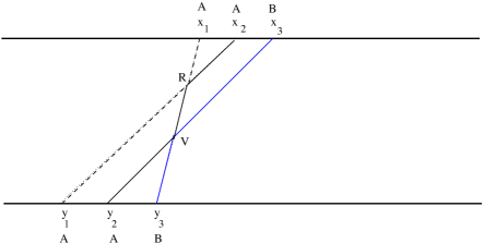
Figure 3: The sequence $AAB$ remains same in time and the $AB$ pair must behave like VRW.

Consider another example. In Fig 4 in the collision $I$ the $A$ and $B$ interchange and in collision $R$ the line $(x_{2}-y_{1})$ has a backward reflection and $(x_{1}-y_{3})$ has forward reflection. These taken together yields $F_{1}(x_{2}-y_{1})\left[F_{-1}(x_{1}-y_{3})F_{0}(x_{3}-y_{2})-F_{-1}(x_{3}-y_{2})F_{0}(x_{1}-y_{3})\right]$. Note that the part in the square bracket has the same form as in Eq. (66) but because $(x_{1}-y_{3})$ suffers a forward reflection with $(x_{2}-y_{1})$, its index is lowered by unity.

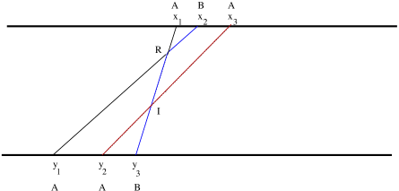
Figure 4: Sequence $AAB$ changes to $ABA$ and in the collision marked $I$ the $AB$ pair actually interchange and collision $R$ is of reflecting type

Note that not all the $N!$ diagrams are always allowed. In the above example, when an initial sequence $AAB$ changed to $ABA$, then not all diagrams are possible: Since we want the $B$ particle starting at $y_{3}$ to interact with the other $A$ particles, we cannot have any diagram where $x_{3}$ is joined to $y_{3}$, meaning no intersection lies on the $(x_{3}-y_{3})$ line. In Bethe Ansatz language this means that all permutations where $p_{3}x_{3}$ appears are absent from the solution.

Thus these diagrams serve as an alternative way to interpret the terms in the Bethe Ansatz solution. This approach also offers us an insight into the theorem discussed in section III. We can now understand why the determinant in Schu97 for the single species case gets modified into $\det G$ for the two-species case obtained above. When only one type of particles is present, the intersections in their trajectories result in only reflecting type collisions and the corresponding index of the $F$ function is either $+1$ or $-1$. It can be easily seen that the line $(x_{i}-y_{j})$ picks up an index $(i-j)$ for the $F$ function, as a result of all these reflections. But when both $A$ and $B$ particles are present, and if we are interested in the case when their sequence do not change, then some of these collisions have to be of ‘vicious’ type which corresponds to an index $0$. For the line $(x_{i}-y_{j})$ the number of such ‘vicious’ collisions is $n_{AB}$, the number of $AB$ pairs between the $i$-th and $j$-th particle. As a result, the corresponding index of the $F$ function is not $(i-j)$ but $sgn(i-j)(|i-j|-n_{AB})$. This explains the structure of the matrix $G$ in section III.

V Further Discussion

In this paper we have used the Bethe Ansatz to solve the master equation of the TASEP with first and second class particles for arbitrary initial conditions. We have also obtained a compact determinantal representation of the solution for the case when the initial sequence of particles remains unchanged. An equivalent geometrical approach developed in section IV provides us with insight into the form of the determinant. We have seen that when the sequence does not change with time, then all the $AB$ pairs in the sequence must behave like VRWs.

Interestingly the last conclusion remains valid even when more than two species of particles are present in the system. For any initial sequence $Q$, consisting of any arbitrary number of species (classes) of particles, if we are interested in the probability that the sequence does not change until time $t$, then all the pairs, where a higher class particle has a lower class particle to its right, must behave like VRWs. All the trajectories where they jump onto each other, must therefore be forbidden because once they interchange positions, they cannot go back again. Generalizing the geometrical approach of section IV, it is easy to see that even in this case the diagrams contain two different types of intersection points: one of vicious type (corresponding to an index $0$) and the other of reflecting type (corresponding to an index $\pm 1$). For any given line $(x_{i}-y_{j})$, there will be an $F$ function as before, with the argument $(x_{i}-y_{j})$ and index $n(i,j)=sgn(i-j)(|i-j|-n_{v})$ where $n_{v}$ denotes the number of ‘vicious pairs’ (where a higher class particle has a lower class particle on its right) between $i$-th and $j$-th member of the sequence. Thus using this approach one can write down a determinantal representation for the solution of the master equation for a general multi-class TASEP where the sequence of various species of particles remains unchanged.

In the special case of a sequence where the first particle from the left is of class $1$, the second particle is of class $2$, the third particle is of class $3$, …,the $N$-th particle is of class $N$, it follows from the above argument that all the pairs in this sequence behave like VRW’s if we consider the probability that the sequence is preserved until time $t$. This probability is nothing but $\det F^{0}$ where $F^{0}$ is a matrix with $(ij)$-th element ${F^{0}}_{ij}=F_{0}(x_{i}-y_{j})$. If on the other hand the initial sequence is reversed when the first class particle becomes the rightmost particle and the $N$-th class particle becomes the leftmost particle, then there are no vicious pairs left in the system and the solution for the single species TASEP remains valid. Thus depending on the labels of the particles in the initial sequence, one can have TASEP solution or VRW solution.

In this context it is interesting to discuss another recent result on the crossover from VRW to TASEP. In semi a model for semi-vicious walkers was introduced that interpolates between VRW and TASEP, having the two as limiting cases. In this model two particles annihilate if they jump on each other, but this jump attempt to an occupied site takes place with a reduced probability. Note that for VRW’s the probability to jump on an occupied site is same as that for an empty site, while for the TASEP jumping on an occupied site is prohibited. Thus by varying the probability to jump on an occupied site one can go from one limiting case to the other and the model for semi-vicious walkers serves an intermediate between these two limits. It was shown that the survival probability for $N$ particles can be described by a scaling form that characterizes the transition from VRW to TASEP semi . In contrast we consider here a multi-species exclusion process and have argued in the previous paragraph that if each of the $N$ particles belongs to a distinct class, then it is possible to have a VRW or a TASEP solution depending on the label of the particles in the initial sequence. For a general sequence, under the condition that until time $t$ the sequence remains unchanged, some of the particles behave like TASEP and some behave like VRW. Thus both these aspects are simultaneously present in our model. In the case when the number of vicious interfaces $n_{v}=N-1$, all the particles behave like VRW and the solution of the master equation becomes $\det F^{0}$, while for $n_{v}=0$ all the particles behave as TASEP particles. For intermediate values of $n_{v}$ both these limiting behaviors are present and some pairs behave like TASEP and some like VRW and the determinantal solution of the master equation is modified accordingly.

For the general two-species problem, i.e. when the initial sequence of species changes because of interchange of $A$ and $B$ particles, it is an interesting question whether the Bethe ansatz solution presented in this work allows for a compact representation in terms of determinants. At this point we do not have a complete answer to this question. We have been able to obtain compact representations for certain special cases. For example, if the final sequence $Q^{\prime}$ results from a single $AB$ interchange from the initial sequence $Q$, such that the number of $AB$ pairs in $Q^{\prime}$ is less than that in $Q$, then we have been able to prove that the probability $P^{Q^{\prime}|Q}=P^{Q^{\prime}|Q^{\prime}}-P^{Q|Q}$ can be written as a difference of two determinants. The existence of similar compact representation for any number of interchanges and for the general multi-class TASEP is an open problem for future investigation.

VI Acknowledgments

We acknowledge useful discussions with V.B. Priezzhev, T. Sasamoto, P.L. Ferrari, A. Rákos, P. Gonçalves. Financial support from Deutsche Forschunsgemeinschaft is gratefully acknowledged.

Appendix A Verification of Yang-Baxter Criterion

In this appendix, we discuss the validity of Yang-Baxter equation for $N=3$ case. Consider the r.h.s. of Eq. (17). The matrices $\Sigma_{12}^{3}(p_{j},p_{k})$ and $\Sigma_{23}^{3}(p_{j},p_{k})$ represents elementary permutations of the momenta variables. For example, $\Sigma_{12}^{3}(p_{j},p_{k})$ represents the interchange of the momentum variables $p_{j}$ and $p_{k}$ which are coupled to $x_{1}$ and $x_{2}$, respectively. Each term in Eq. (17) corresponds to one particular permutation ${\cal P}$ of the momenta and the product of the $\Sigma$ matrices represents decomposition of ${\cal P}$ into a series of elementary permutations. This decomposition need not be unique for all ${\cal P}$. Consider, for example, the last term in Eq. (17), where the momenta variables coupled to $x_{1},x_{2},x_{3}$, are, respectively, $p_{3},p_{2},p_{1}$. Starting from a permutation $p_{1},p_{2},p_{3}$ (as in the first term on the r.h.s. of Eq. (17), to reach the arrangement $p_{3},p_{2},p_{1}$, one can first interchange $(p_{2},p_{3})$, then $(p_{1},p_{3})$ and again $(p_{1},p_{2})$. Accordingly, the $\Sigma$-product is $\Sigma_{23}^{3}(p_{1},p_{2})\Sigma_{12}^{3}(p_{1},p_{3})\Sigma_{23}^{3}(p_{2},p_{3})$. But the same permutation can also be reached by first interchanging $(p_{1},p_{2})$, then $(p_{1},p_{3})$ and finally $(p_{2},p_{3})$. In that case, the corresponding matrix will be $\Sigma_{12}^{3}(p_{2},p_{3})\Sigma_{23}^{3}(p_{1},p_{3})\Sigma_{12}^{3}(p_{1},p_{2})$. In order for the system to be integrable, one must satisfy the Yang-Baxter criterion

$$\Sigma_{12}^{3}(p_{2},p_{3})\Sigma_{23}^{3}(p_{1},p_{3})\Sigma_{12}^{3}(p_{1},p_{2})=\Sigma_{23}^{3}(p_{1},p_{2})\Sigma_{12}^{3}(p_{1},p_{3})\Sigma_{23}^{3}(p_{2},p_{3}).$$ (67)

(We remark that the slightly different Yang-Baxter equation for the scattering matrix $S$ is obtained from this croterion through the relation $S=\Sigma P$ where $P$ is the permutation operator). Now, using the definitions $\Sigma_{12}^{3}(p_{j},p_{k})\equiv\Sigma(p_{j},p_{k})\otimes{\mathbb{I}}_{2}$ and $\Sigma_{23}^{3}(p_{j},p_{k})\equiv{\mathbb{I}}_{2}\otimes\Sigma(p_{j},p_{k})$, we have

$$\Sigma_{12}^{3}(p_{i},p_{j})=\left(\begin{array}[]{cccccccc}S_{jk}&0&0&0&0&0&0&0\\ 0&S_{jk}&0&0&0&0&0&0\\ 0&0&-1&0&0&0&0&0\\ 0&0&0&-1&0&0&0&0\\ 0&0&T_{jk}&0&S_{jk}&0&0&0\\ 0&0&0&T_{jk}&0&S_{jk}&0&0\\ 0&0&0&0&0&0&S_{jk}&0\\ 0&0&0&0&0&0&0&S_{jk}\end{array}\right)$$ (68)

and

$$\Sigma_{23}^{3}(p_{i},p_{j})=\left(\begin{array}[]{cccccccc}S_{jk}&0&0&0&0&0&0&0\\ 0&-1&0&0&0&0&0&0\\ 0&T_{jk}&S_{jk}&0&0&0&0&0\\ 0&0&0&S_{jk}&0&0&0&0\\ 0&0&0&0&S_{jk}&0&0&0\\ 0&0&0&0&0&-1&0&0\\ 0&0&0&0&0&T_{jk}&S_{jk}&0\\ 0&0&0&0&0&0&0&S_{jk}\end{array}\right)$$ (69)

where $S_{jk}=-(1-e^{ip_{j}})/(1-e^{ip_{k}})$ and $T_{jk}=-(e^{ip_{k}}-e^{ip_{j}})/(1-e^{ip_{k}})$. Using these forms it is straightforward to verify Eq. (67).

We remark that the nested Bethe ansatz can be also be used for treating second-class particles in the partially asymmetric simple exclusion process (PASEP) where particles jump to the right or left with non-zero rates arita . However, even for the single-species PASEP there is no known determinantal representation of the transition probabilities.

References

• (1) Liggett TM Stochastic interacting systems: contact, voter and exclusion processes (Springer, Berlin, 1999)
• (2) G.M. Schütz, in C.Domb and J.Lebowitz (eds.) Phase Transitions and Critical Phenomena, Vol.19 (Academic, London, pp.1-251, 2001).
• (3) H. Spohn, Large Scale Dynamics of Interacting Particles, (Springer, Berlin, 1991).
• (4) J.M. Burgers, The Nonlinear Diffusion Equation (Riedel, Boston, 1974).
• (5) M. Kardar, G. Parisi, Y-C. Zhang, Phys. Rev. Lett. 56, 889 (1986).
• (6) T. Sasamoto, H. Spohn, arXiv:1002.1879 (2010).
• (7) O. Angel, J. Combin. Theory Ser. A 113 625 (2006).
• (8) P. Ferrari, C. Kipnis and E. Saada, Ann. Prob. 19, 226 (1991).
• (9) P. A. Ferrari and L. R. G. Fontes, Probab. Theory Relat. Fields 99, 305 (1994).
• (10) B. Derrida, J. L. Lebowitz and E. Speer, J. Stat. Phys. 89, 135 (1997).
• (11) V. Belitsky and G.M. Schütz, El. J. Prob. 7, 11 (2002).
• (12) K. Krebs, F.H. Jafarpour and G.M. Schütz, New J. Phys. 5, 145 (2003).
• (13) E.R. Speer in C. Fannes and A. Verbuere (eds.) On Three Levels: Micro, Meso and Macroscopic Approaches in Physics (Plenum, New York, pp.91-102, 1994).
• (14) B. Derrida, S. A. Janowsky, J. L. Lebowitz and E. R. Speer, Europhys. Lett. 22, 651 (1993).
• (15) C. Godrechè et al., J. Phys. A: Math. Gen. 28 6039 (1995).
• (16) G.M. Schütz, J. Phys. A: Math. Gen. 36 R339 (2003).
• (17) R.A. Blythe and M.R. Evans, J. Phys. A: Math. Theor. 40 R333 (2007).
• (18) K. Johansson, Commun. Math. Phys. 209(2), 437-476 (2000).
• (19) P.A. Ferrari, P. Gonçalves and J.B. Martin, Ann. Inst. H. Poincaré Probab. Statist. 45 1048 (2009).
• (20) P.A. Ferrari and J.B. Martin, Ann. Prob. 35 807 (2007).
• (21) M.R. Evans, P.A. Ferrari and K. Mallick, J. Stat. Phys. 135 217 (2009).
• (22) G.M. Schütz, J. Stat. Phys. 88, 427 (1997).
• (23) L.H. Gwa and H. Spohn, Phys. Rev. Lett. 68 725 (1992).
• (24) T. Nagao and T. Sasamoto, Nucl. Phys. B 699(3), 487-502 (2004).
• (25) A. Rákos and G.M. Schütz, J. Stat. Phys. 118 (3-4): 511 - 530 (2005).
• (26) V.B. Priezzhev and G.M. Schütz, J. Stat. Mech.: Theor. Exp. P09007 (2008)
• (27) J. Brankov, V.B. Priezzhev and R. V. Shelest, Phys. Rev. E 69, 066136 (2004).
• (28) T. Sasamoto, J. Phys. A : Math. Gen. 38, L549-L556 (2005).
• (29) A.M. Povolotsky and V.B. Priezzhev, J. Stat. Mech., P07002 (2006).
• (30) T. Sasamoto, J. Stat. Mech., P07007 (2007).
• (31) A. Borodin, P.L. Ferrari , M. Prähofer and T. Sasamoto, J. Stat. Phys. 129 (5-6), 1055-1080 (2007).
• (32) A. Borodin and P.L. Ferrari, El. J. Prob. 13, 1380-1418 (2008).
• (33) C.A. Tracy and H. Widom, Commun. Math. Phys. 279(3) 815-844 (2008).
• (34) C.A. Tracy and H. Widom, J. Stat. Phys. 132(2), 291-300 (2008).
• (35) C.L. Schultz, Physica 122A 71 (1983).
• (36) C.N. Yang, Phys. Rev. Lett. 19 1312 (1967).
• (37) B. Sutherland, Phys. Rev. Lett. 20 98 (1968).
• (38) C. Arita, A. Kuniba, K. Sakai and T. Sawabe, J. Phys. A: Math. Theor. 42 345002 (2009).
• (39) F. C. Alcaraz and V. Rittenberg, Phys. Lett. B 314, 377 (1993).
• (40) V. Popkov, E. Fouladvand, and G.M. Schütz, J. Phys. A: Math. Gen. 35 7187-7204 (2002).
• (41) V.B. Priezzhev, Phys. Rev. Lett. 91 050601 (2003).
• (42) V.B. Priezzhev, Phys. Rev. E 69 066136 (2004).
• (43) A.A. Lushnikov, Sov. Phys. JETP 64 811 (1986) and Phys. Lett. A 120 135 (1987).
• (44) M. Barma, M.D. Grynberg and R.B. Stinchcombe, Phys. Rev. Lett. 70 1033 (1993).
• (45) R.B. Stinchcombe, M.D. Grynberg and M. Barma, Phys. Rev. E 47 4018 (1993).
• (46) G. M. Schütz, J. Phys. A 28, 3405 (1995).
• (47) T.C. Dorlas, A.M. Povolotsky and V.B. Priezzhev, J. Stat. Phys. 135 483 (2009).