Non–abelian gauge structure in neutrino mixing

Abstract

We discuss the existence of a non–abelian gauge structure associated with flavor mixing. In the specific case of two flavor mixing of Dirac neutrino fields, we show that this reformulation allows to define flavor neutrino states which preserve the Poincaré structure. Phenomenological consequences of our analysis are explored.

I Introduction

The study of neutrino mixing and oscillations is of utmost importance in contemporary theoretical and experimental physics, due to the experimental discovery of neutrino oscillations. At a theoretical level, one important issue is the one of a correct definition of the flavor states i.e. the ones describing oscillating neutrinos. In the standard quantum mechanical treatment, the well known Pontecorvo states Bilenky:1978nj are used and oscillation formulas are derived, which can describe efficiently the main aspects of such a phenomenon. However, it is clear that Pontecorvo states are only approximate since they are not eigenstates of the flavor neutrino charges. Thus Pontecorvo states lead to violation of the conservation of leptonic charge in the neutrino production vertices BCTV2005 ; Nishi:2008sc .

The solution to the above problem has been found in the context of Quantum Field Theory (QFT). Indeed, by considering mixing at level of fields, rather than postulating it as a property of states, unexpected features emerged BV95 . It has been found that field mixing is associated with inequivalent representation of the canonical anticommutation relations, i.e. the vacuum for the mass eigenstates of neutrinos has been found to be unitarily inequivalent to the vacuum for the flavor eigenstates of neutrinos – the flavor vacuum. The nonperturbative vacuum structure associated with field mixing has been found to be a very general feature, independently of the nature of the fields Ji ; Fujii:1999xa ; bosonmix ; 3flav ; Blasone:2003hh . It has also been shown that it leads to modifications of the flavor oscillation formulae BHV98 ; Blasone:2002wp ; Ji ; Fujii:1999xa .

In QFT flavor states can be straightforwardly defined as eigenstates of the flavor charges which are derived in a canonical way from the symmetry properties of the neutrino Lagrangian BJV01 . It has been shown that states defined in this way restore flavor charge conservation in weak interaction vertices, at tree level Blasone:2006jx . Moreover, such states turn out to be eigenstates of the momentum operator.

Despite the above mentioned results, the QFT treatment of flavor states still presents some open problems. One such issue is Lorentz invariance. Indeed, the flavor vacuum is not Lorentz invariant being explicitly time-dependent. As a consequence, flavor states cannot be interpreted in terms of irreducible representations of the Poincaré group. A possible way to recover Poincaré invariance for mixed fields has been explored in Refs.BlaMagueijo where non–standard dispersion relations for the mixed particles have been related to nonlinear realizations of the Poincaré group MagSmol . Another interesting issue concerns the invariance of the flavor oscillation formulas under Lorentz boosts Blasone:2005tm .

The relation of neutrino masses and mixing with a possible violation of the Poincaré and $CPT$ symmetries has been the subject of many efforts in the last decade Pakvasa:2001yw . A related line of research concerns the use of neutrino mixing and oscillations as a sensitive probe for quantum gravity effects, as quantum gravity induced decoherence is expected to affect neutrino oscillations AmelinoCamelia:2007kx . Such effects have also been connected Mavromatos:2007ak to the non trivial structure of the flavor vacuum introduced in BV95 .

In this paper we propose an approach to the mixing of particles which overcomes the problems mentioned above. The basic idea is to view the mixing phenomenon as the result of the interaction of the neutrino fields with an external field, which as we shall see appears to be a non-abelian gauge field. This point of view allows to treat formally the mixed fields as free fields, avoiding in this way the problems with their interpretation in terms of the Poincaré group. The violation of relativistic invariance is now seen as a consequence of the presence of a fixed external field, which defines a preferred direction in spacetime.

Our approach enables us to define flavor neutrino states which are simultaneous eigenstates of the flavor charges, of the momentum operators and of a new Hamiltonian operator for the mixed fields whose definition naturally emerges from our approach. This operator can be interpreted as the energy which can be extracted from flavor neutrinos through scattering. We discuss a possible test for our theoretical scheme, by looking at mixed neutrinos in the $\beta$ decay, where the endpoint of the electron energy spectrum turns out to be different in our approach with respect to the standard prediction.

In the present paper, we consider only the mixing of two Dirac fermion fields. Similar results hold also for the case of mixing of boson fields, and for the case of three flavors. An analysis of these instances will be presented elsewhere.

II Two-flavor neutrino mixing

We begin with the Lagrangian density describing two mixed neutrino fields:

$${\cal L} = {\bar{\nu}}_{e}\left(i\not\!\partial-m_{e}\right)\nu_{e}+{\bar{\nu}}_{\mu}\left(i\not\!\partial-m_{\mu}\right)\nu_{\mu}\,-\,m_{e\mu}\,\left({\bar{\nu}}_{e}\,\nu_{\mu}\,+\,{\bar{\nu}}_{\mu}\,\nu_{e}\right).$$ (1)

The standard treatment of the problem is based on the observation that this Lagrangian, being quadratic, can be diagonalized by a canonical transformation of the field operators (called the mixing transformation):

$$\nu_{e} = \nu_{1}\cos\theta+\nu_{2}\sin\theta$$ (2)

$$\nu_{\mu} = -\nu_{1}\sin\theta+\nu_{2}\cos\theta,$$ (3)

so that one simply gets the sum of two free Dirac Lagrangians:

$${\cal L} = {\bar{\nu}}_{1}\left(i\not\!\partial-m_{1}\right)\nu_{1}+{\bar{\nu}}_{2}\left(i\not\!\partial-m_{2}\right)\nu_{2}.\;$$ (4)

In the above equations, $\theta$ is the mixing angle and $m_{e}=m_{1}\cos^{2}\theta+m_{2}\sin^{2}\theta$, $m_{\mu}=m_{1}\sin^{2}\theta+m_{2}\cos^{2}\theta$, $m_{e\mu}=(m_{2}-m_{1})\sin\theta\cos\theta\,$.

From the above lagrangian, one can derive the canonical energy-momentum tensor:

$$T_{\rho\sigma} = {\bar{\nu}}_{e}i\gamma_{\rho}\partial_{\sigma}\nu_{e}-\eta_{\rho\sigma}{\bar{\nu}}_{e}(i\gamma^{\lambda}\partial_{\lambda}-m_{e})\nu_{e}+{\bar{\nu}}_{\mu}i\gamma_{\rho}\partial_{\sigma}\nu_{\mu}-\eta_{\rho\sigma}{\bar{\nu}}_{\mu}(i\gamma^{\lambda}\partial_{\lambda}-m_{\mu})\nu_{\mu}+\eta_{\rho\sigma}m_{e\mu}({\bar{\nu}}_{e}\nu_{\mu}+{\bar{\nu}}_{\mu}\nu_{e})$$ (5)

$$= {\bar{\nu}}_{1}i\gamma_{\rho}\partial_{\sigma}\nu_{1}-\eta_{\rho\sigma}{\bar{\nu}}_{1}(i\gamma^{\lambda}\partial_{\lambda}-m_{1})\nu_{1}+{\bar{\nu}}_{2}i\gamma_{\rho}\partial_{\sigma}\nu_{2}-\eta_{\rho\sigma}{\bar{\nu}}_{2}(i\gamma^{\lambda}\partial_{\lambda}-m_{2})\nu_{2},$$

where $\eta_{\rho\sigma}=\textrm{diag}(+1,-1,-1,-1)$ is the Minkowskian metric tensor. From this tensor it follows the total Hamiltonian:

$${H} = \int d^{3}\mathbf{x}\,{T}^{00}=\int d^{3}\mathbf{x}\,\nu_{1}^{\dagger}\left(-i{\bm{\alpha}}\cdot{\bm{\nabla}}+\beta m_{1}\right)\nu_{1}+\int d^{3}\mathbf{x}\,\nu_{2}^{\dagger}\left(-i{\bm{\alpha}}\cdot{\bm{\nabla}}+\beta m_{2}\right)\nu_{2}.$$ (6)

which is just the sum of the two free field Hamiltonians: $H=H_{1}+H_{2}$.

Analogously, a momentum operator is defined as:

$${P}^{i} = \int d^{3}\mathbf{x}\,{T}^{0i}\,=\,i\int d^{3}\mathbf{x}\,\nu_{1}^{\dagger}\partial^{i}\nu_{1}+i\int d^{3}\mathbf{x}\,\nu_{2}^{\dagger}\partial^{i}\nu_{2},\qquad i=1,2,3$$ (7)

which again is the sum of two free field contributions.

To the free fields $\nu_{i}$ there are associated two conserved (Noether) charges:

$$Q_{j}\,=\,\int d^{3}{\bf x}\,\nu_{j}^{{\dagger}}(x)\;\nu_{j}(x)\,,\qquad j=1,2,$$ (8)

with the total charge $Q=Q_{1}+Q_{2}$. The analysis of symmetries of the Lagrangian in the flavor basis Eq.(1), leads to the identification of the (non conserved) flavor charges BJV01 :

$$Q_{\sigma}(x_{0})\,=\,\int d^{3}{\bf x}\,\nu_{\sigma}^{{\dagger}}(x)\;\nu_{\sigma}(x)~{},\quad\sigma=e,\mu,$$ (9)

with $Q_{e}(x_{0})+Q_{\mu}(x_{0})=Q$. Flavor charges describe the phenomenon of neutrino oscillations, see Appendix A.

It is interesting to consider the relation among the two sets of charges:

$$Q_{e}(x_{0}) = \cos^{2}\theta\;Q_{1}+\sin^{2}\theta\;Q_{2}+\sin\theta\cos\theta\int d^{3}{\bf x}\left[\nu_{1}^{\dagger}(x)\nu_{2}(x)+\nu_{2}^{\dagger}(x)\nu_{1}(x)\right]\,,$$ (10)

$$Q_{\mu}(x_{0}) = \sin^{2}\theta\;Q_{1}+\cos^{2}\theta\;Q_{2}-\sin\theta\cos\theta\int d^{3}{\bf x}\left[\nu_{1}^{\dagger}(x)\nu_{2}(x)+\nu_{2}^{\dagger}(x)\nu_{1}(x)\right]\,.$$ (11)

The appearance of terms that cannot be written in terms of $Q_{j}$ is related to a non-trivial structure of the flavor Hilbert space BV95 , see Appendix A.

III Flavor mixing as a non-abelian gauge theory

We now show that the Lagrangian Eq.(1) can be formally written as a non-abelian gauge theory. In the following we shall use the conventions of Ref. LeiteLopes:1981fr .

The starting point is the observation that the mixing interaction can be consistently viewed as the interaction of the flavor neutrino fields with a constant external gauge field. The most direct way of seeing this goes through the Euler–Lagrange equations corresponding to the Lagrangian (1), namely:

$$i\partial_{0}\nu_{e} = (-i{\bm{\alpha}}\cdot{\bm{\nabla}}+\beta m_{e})\nu_{e}+\beta m_{e\mu}\nu_{\mu}$$ (12)

$$i\partial_{0}\nu_{\mu} = (-i{\bm{\alpha}}\cdot{\bm{\nabla}}+\beta m_{\mu})\nu_{\mu}+\beta m_{e\mu}\nu_{e},$$ (13)

where $\alpha_{i}$, $i=1,2,3$ and $\beta$ are the usual Dirac matrices in a given representation. Here we choose the following representation:

$$\alpha_{i}=\left(\begin{array}[]{cc}0&\sigma_{i}\\ \sigma_{i}&0\end{array}\right),\qquad\beta=\left(\begin{array}[]{cc}1{\rm I}&0\\ 0&-1{\rm I}\end{array}\right),$$ (18)

where $\sigma_{i}$ are the Pauli matrices and $1{\rm I}$ is the $2\times 2$ identity matrix. The Euler–Lagrange equations can be compactly written as follows:

$$iD_{0}\nu_{f}=(-i{\bm{\alpha}}\cdot{\bm{\nabla}}+\beta M_{d})\nu_{f},$$ (19)

where $\nu_{f}=(\nu_{e},\nu_{\mu})^{T}$ is the flavor doublet and $M_{d}={\rm diag}(m_{e},m_{\mu})$ is a diagonal mass matrix. We have defined the (non-abelian) covariant derivative:

$$D_{0}:=\partial_{0}+i\,m_{e\mu}\,\beta\,\sigma_{1},$$ (20)

where $m_{e\mu}=\frac{1}{2}\,\tan 2\theta\,\delta m$, and $\delta m:=m_{\mu}-m_{e}$.

We thus see that flavor mixing can be seen as an interaction of the flavor fields with an $SU(2)$ constant gauge field having the following structure:

$$A_{\mu} := \frac{1}{2}A_{\mu}^{a}\sigma_{a}\,=\,n_{\mu}\delta m\,\frac{\sigma_{1}}{2}\in su(2),\qquad n^{\mu}:=(1,0,0,0)^{T},$$ (21)

that is, having only the temporal component in spacetime and only the first component in $su(2)$ space. In terms of this connection, the covariant derivative can be written in the form:

$$D_{\mu}=\partial_{\mu}+i\,g\,\beta\,A_{\mu},$$ (22)

where we have defined $g:=\tan 2\theta$ as the coupling constant for the mixing interaction. Note that in the case of maximal mixing ($\theta=\pi/4$), the coupling constant grows to infinity while $\delta m$ goes to zero. We further note that, since the gauge connection is a constant, with just one non-zero component in group space, its field strength vanishes identically:

$$F_{\mu\nu}^{a}=\epsilon^{abc}A_{\mu}^{b}A_{\nu}^{c}=0,$$ (23)

with $a,b,c=1,2,3$. The fact that, despite $F_{\mu\nu}$ vanishes identically, the gauge field has physical effects, leads to an analogy with the Aharonov–Bohm effect Aharonov:1959fk .

Finally, the equations of motion for the mixed fields can be cast in a manifestly covariant form:

$$(i\gamma^{\mu}D_{\mu}-M_{d})\nu_{f}=0,$$ (24)

and the Lagrangian density (1) has the form of the one describing a doublet of Dirac fields in interaction with an external Yang-Mills field:

$${\cal L}={\bar{\nu}}_{f}(i\gamma^{\mu}D_{\mu}-M_{d})\nu_{f}.$$ (25)

III.1 Energy-momentum tensor and 4-momentum operator

In this Section we study the energy momentum tensor associated with the flavor neutrino fields in interaction with the external gauge field. This object can be computed by means of the standard procedure LeiteLopes:1981fr . One finds:

$$\widetilde{T}_{\rho\sigma}={\bar{\nu}}_{f}i\gamma_{\rho}D_{\sigma}\nu_{f}-\eta_{\rho\sigma}{\bar{\nu}}_{f}(i\gamma^{\lambda}D_{\lambda}-M_{d})\nu_{f}.$$ (26)

This expression is to be compared with the one of the canonical energy momentum tensor given in Eq.(5) from which we see that the difference between the two is just the presence of the interaction terms in the $00$ component, i.e. $T_{00}-\widetilde{T}_{00}=m_{e\mu}({\bar{\nu}}_{e}\nu_{\mu}+{\bar{\nu}}_{\mu}\nu_{e})$, while we have $T_{0i}=\widetilde{T}_{0i}$, $T_{ij}=\widetilde{T}_{ij}$.

The tensor $\widetilde{T}_{\mu\nu}$ is not conserved on-shell. In particular we have:

$$\partial^{\rho}\widetilde{T}_{\rho i}\,=\,0;\qquad\quad\partial^{\rho}\widetilde{T}_{\rho 0}\neq 0.$$ (27)

Note that without the $\beta$ matrix appearing in the covariant derivative (20) we would have found: $\partial^{\mu}\widetilde{T}_{\mu\nu}=gF_{\mu\nu a}j^{\mu}_{a}\,=\,0,$ i.e. the energy-momentum tensor would have been conserved. In the present case $[\gamma_{\mu},D_{0}]\neq 0$, in consequence of the presence of the $\beta$ matrix in $D_{0}$.

We also note that the matter current $j^{\mu}_{a}$ has only one component in group space:

$$j^{\rho}_{1}={\bar{\nu}_{f}}\gamma^{\rho}\frac{\sigma_{1}}{2}\nu_{f}=\frac{1}{2}({\bar{\nu}_{e}}\gamma^{\rho}\nu_{\mu}+{\bar{\nu}_{\mu}}\gamma^{\rho}\nu_{e})=J^{\rho}_{f,1},$$ (28)

where $J^{\rho}_{f,1}$ is the Noether current associated to the Lagrangian density (25) under the $SU(2)$ transformation BJV01 :

$$\nu_{f}^{\prime}=e^{im_{e\mu}\lambda_{1}\frac{\sigma_{1}}{2}}\nu_{f}.$$ (29)

Following the usual procedure, we now define a $4$-momentum operator $\widetilde{P}^{\mu}$ by taking the $0i$ and $00$ components of $\widetilde{T}^{\mu\nu}$ and integrating them over $3-$space. We obtain a conserved $3-$momentum operator:

$$\widetilde{P}^{i} = \int d^{3}\mathbf{x}\,\widetilde{T}^{0i}=i\int d^{3}\mathbf{x}\,\nu_{f}^{\dagger}\partial^{i}\nu_{f}$$ (30)

$$= i\int d^{3}\mathbf{x}\,\nu_{e}^{\dagger}\partial^{i}\nu_{e}+i\int d^{3}\mathbf{x}\,\nu_{\mu}^{\dagger}\partial^{i}\nu_{\mu}$$

$$\equiv \widetilde{P}^{i}_{e}(x_{0})+\widetilde{P}^{i}_{\mu}(x_{0}),\qquad\qquad\qquad\qquad i=1,2,3$$

and a non conserved Hamiltonian operator:

$$\widetilde{P}^{0}(x_{0})\equiv\widetilde{H}(x_{0}) = \int d^{3}\mathbf{x}\,\widetilde{T}^{00}=\int d^{3}\mathbf{x}\,{\bar{\nu}}_{f}\left(i\gamma_{0}D_{0}-i\gamma^{\mu}D_{\mu}+M_{d}\right)\nu_{f}$$ (31)

$$= \int d^{3}\mathbf{x}\,\nu_{e}^{\dagger}\left(-i{\bm{\alpha}}\cdot{\bm{\nabla}}+\beta m_{e}\right)\nu_{e}+\int d^{3}\mathbf{x}\,\nu_{\mu}^{\dagger}\left(-i{\bm{\alpha}}\cdot{\bm{\nabla}}+\beta m_{\mu}\right)\nu_{\mu}$$

$$\equiv \widetilde{H}_{e}(x_{0})+\widetilde{H}_{\mu}(x_{0}).$$

We see that both the Hamiltonian and the momentum operators split in a natural way in a contribution involving only the electron neutrino field and in another where only the muon neutrino field appears. In such a way, we have a natural definition of a Hamiltonian and momentum operators for each flavor field.

We remark that the tilde Hamiltonian is not the generator of time translations. This role competes to the complete Hamiltonian $H=\int d^{3}\mathbf{x}\,T^{00}$, which includes the interaction term.

IV Flavor neutrino states and Lorentz invariance

Till now our considerations have been purely classical. Now we want to pass to the quantum theory. Our purpose is to construct flavor neutrino states which are simultaneous eigenstates of the $4-$momentum operators above constructed and of the flavor charges. Of course this is a highly nontrivial request. We will see that such states can indeed be constructed, but this involves a nontrivial redefinition of the flavor vacuum which will also erase any reference to the $\nu_{1}$ and $\nu_{2}$ fields.

As shown in Appendix A, the flavor neutrino field operators can be expanded in the same basis as the free fields with masses $m_{1}$ and $m_{2}$:

$$\nu_{\sigma}(x)=\int\frac{d^{3}\mathbf{k}}{(2\pi)^{3/2}}\sum_{r}\left[u^{r}_{\mathbf{k},j}(x_{0})\alpha^{r}_{\mathbf{k},\sigma}(x_{0})+v^{r}_{-\mathbf{k},j}(x_{0})\beta^{r\dagger}_{\mathbf{-k},\sigma}(x_{0})\right]e^{i\mathbf{k}\cdot\mathbf{x}},\qquad(\sigma,j)=(e,1)(\mu,2),$$ (32)

where $\alpha_{\mathbf{k},\sigma}$ and $\beta_{\mathbf{-k},\sigma}$ are the flavor ladder operators BV95 . In the same Appendix we show that flavor neutrino states, defined as $|\nu^{r}_{\mathbf{k},\sigma}\rangle=\alpha^{r{\dagger}}_{\mathbf{k},\sigma}|0\rangle_{e,\mu}$, are eigenstates of the flavor charge operators $Q_{\sigma}$, at a given time. They turn out also to be eigenstates of the momentum operators $P^{i}=\int d^{3}\mathbf{x}\,T^{0i}$. However, since the Hamiltonian operator $H$ does not commute with the charges $Q_{\sigma}$, the above flavor states do not have definite energies.

We will now show that this problem can be solved by noting that the expansion (32) actually relies on a special choice of the bases of spinors, namely those referring to the free field masses $m_{1}$, $m_{2}$. It is however always possible to perform a Bogoliubov transformation in order to expand the field operators in a different basis of spinors, referring to an arbitrarily chosen couple of mass parameters Fujii:1999xa . Let $\mu_{\sigma}$, $\sigma=e,\mu$ be such a couple of arbitrary parameters.

The Bogoliubov transformation to be performed is the following:

$$\left(\begin{array}[]{c}\widetilde{\alpha}_{\mathbf{k},\sigma}^{r}(x_{0})\\ \widetilde{\beta}_{-\mathbf{k},\sigma}^{r\dagger}(x_{0})\end{array}\right)=J^{-1}_{\mu}(x_{0})\left(\begin{array}[]{c}\alpha_{\mathbf{k},\sigma}^{r}(x_{0})\\ \beta_{-\mathbf{k},\sigma}^{r\dagger}(x_{0})\end{array}\right)J_{\mu}(x_{0}),$$ (37)

where the generator is Fujii:1999xa :

$$J_{\mu}(x_{0})=\prod_{\mathbf{k},r}\exp\left\{i\sum_{(\sigma,j)}\xi^{\mathbf{k}}_{\sigma,j}\left[\alpha_{\mathbf{k},\sigma}^{r\dagger}(x_{0})\beta_{-\mathbf{k},\sigma}^{r\dagger}(x_{0})+\beta_{-\mathbf{k},\sigma}^{r}(x_{0})\alpha_{\mathbf{k},\sigma}^{r}(x_{0})\right]\right\},\qquad(\sigma,j)=(e,1),(\mu,2),$$ (38)

and $\xi^{\mathbf{k}}_{\sigma,j}=(\chi_{\sigma}-\chi_{j})/2$ and $\chi_{\sigma}=\arctan(\mu_{\sigma}/|\mathbf{k}|)$, $\chi_{j}=\arctan(m_{j}/|\mathbf{k}|)$.

The explicit form of the transformation (37) is the following:

$$\left(\begin{array}[]{c}\widetilde{\alpha}_{\mathbf{k},\sigma}^{r}(x_{0})\\ \widetilde{\beta}_{-\mathbf{k},\sigma}^{r\dagger}(x_{0})\end{array}\right)=\left(\begin{array}[]{cc}\rho_{\sigma,j}^{\mathbf{k}}&i\lambda_{\sigma,j}^{\mathbf{k}}\\ i\lambda_{\sigma,j}^{\mathbf{k}}&\rho_{\sigma,j}^{\mathbf{k}}\end{array}\right)\left(\begin{array}[]{c}\alpha_{\mathbf{k},\sigma}^{r}(x_{0})\\ \beta_{-\mathbf{k},\sigma}^{r\dagger}(x_{0})\end{array}\right),\qquad(\sigma,j)=(e,1),(\mu,2),$$ (45)

where $\rho_{\sigma,j}^{\mathbf{k}}=\cos\xi^{\mathbf{k}}_{\sigma,j}$ and $\lambda_{\sigma,j}^{\mathbf{k}}=\sin\xi^{\mathbf{k}}_{\sigma,j}$.

We have thus a whole family of flavor vacua, denoted with a tilde and parameterized by the couples $(\mu_{e},\mu_{\mu})$:

$$|{\widetilde{0}}(x_{0})\rangle_{e\mu}=J_{\mu}^{-1}(x_{0})|0(x_{0})\rangle_{e\mu}.$$ (46)

The original flavor vacuum is of course the one associated with the couple $(m_{1},m_{2})$.

Notice that the flavor charges, as well as the exact oscillation formulae are invariant under the above Bogoliubov transformations remarks , i.e. $\widetilde{Q}_{\sigma}=Q_{\sigma}$, with:

$$\widetilde{Q}_{\sigma}(x_{0})=\sum_{r}\int d^{3}\mathbf{k}\left(\widetilde{\alpha}^{r\dagger}_{\mathbf{k}\sigma}(x_{0})\widetilde{\alpha}^{r}_{\mathbf{k}\sigma}(x_{0})-\widetilde{\beta}^{r\dagger}_{-\mathbf{k}\sigma}(x_{0})\widetilde{\beta}^{r}_{-\mathbf{k}\sigma}(x_{0})\right).$$ (47)

In the context of the above reformulation of mixing as a gauge theory, it seems natural to expand the flavor fields in the bases corresponding to the couple of masses $(m_{e},m_{\mu})$. We will discover that precisely those values are singled out by the requirement that the flavor states be eigenstates of the Hamiltonian operator.

The new spinors are defined as the solutions of the equations:

$$(-\alpha\cdot\mathbf{k}+m_{\sigma}\beta)u^{r}_{\mathbf{k},\sigma} = \omega_{\mathbf{k},\sigma}u^{r}_{\mathbf{k},\sigma}$$ (48)

$$(-\alpha\cdot\mathbf{k}+m_{\sigma}\beta)v^{r}_{-\mathbf{k},\sigma} = -\omega_{\mathbf{k},\sigma}v^{r}_{-\mathbf{k},\sigma},$$ (49)

where $\omega_{\mathbf{k},\sigma}=\sqrt{\mathbf{k}^{2}+m_{\sigma}^{2}}$. These are the momentum space version of the free Dirac equation with mass $m_{\sigma}$.

The flavor field operators are then expanded as follows:

$$\nu_{\sigma}(x)=\int\frac{d^{3}\mathbf{k}}{(2\pi)^{3/2}}\sum_{r}\left[u^{r}_{\mathbf{k},\sigma}(x_{0})\widetilde{\alpha}^{r}_{\mathbf{k},\sigma}(x_{0})+v^{r}_{-\mathbf{k},\sigma}(x_{0})\widetilde{\beta}^{r\dagger}_{\mathbf{-k},\sigma}(x_{0})\right]e^{i\mathbf{k}\cdot\mathbf{x}},\quad\sigma=e,\mu,$$ (50)

with $u^{r}_{\mathbf{k},\sigma}(x_{0})=u^{r}_{\mathbf{k},\sigma}e^{-i\omega_{\mathbf{k},\sigma}x_{0}}$, $v^{r}_{-\mathbf{k},\sigma}(x_{0})=v^{r}_{-\mathbf{k},\sigma}e^{i\omega_{\mathbf{k},\sigma}x_{0}}$. Here and in the following the tilde operators are those corresponding to the specific couple $(m_{e},m_{\mu})$. With these definitions all the calculations at a fixed instant of time $x_{0}$ can be performed in exactly the same way they are done in the free field case. The explicit time dependence of the creation and destruction operators, which is of course due to the interaction with the external field and is not present in the free field case, does not create problems as the states which are acted upon by the operators are evaluated at the same time as the operators themselves and the commutators are all considered at equal times.

In terms of the tilde flavor ladder operators, the Hamiltonian and momentum operators Eqs.(30),(31) read:

$$\widetilde{\mathbf{P}}_{\sigma}(x_{0}) = \sum_{r}\int d^{3}{\bf k}\,\,{\bf k}\left(\widetilde{\alpha}^{r\dagger}_{{\bf k},\sigma}(x_{0})\widetilde{\alpha}^{r}_{{\bf k},\sigma}(x_{0})+\widetilde{\beta}^{r\dagger}_{{\bf{k}},\sigma}(x_{0})\widetilde{\beta}^{r}_{{\bf k},\sigma}(x_{0})\right),$$ (51)

$$\widetilde{H}_{\sigma}(x_{0}) = \sum_{r}\int d^{3}{\bf k}\,\omega_{\mathbf{k},\sigma}\left(\widetilde{\alpha}^{r\dagger}_{{\bf k},\sigma}(x_{0})\,\widetilde{\alpha}^{r}_{{\bf k},\sigma}(x_{0})-\widetilde{\beta}^{r}_{{\bf{k}},\sigma}(x_{0})\,\widetilde{\beta}^{r\dagger}_{{\bf k},\sigma}(x_{0})\right).$$ (52)

The new flavor states are defined by the action of the tilde creation operator on the tilde flavor vacuum:

$$|\widetilde{\nu}^{\,r}_{\mathbf{k},\sigma}(x_{0})\rangle=\widetilde{\alpha}^{r\dagger}_{\mathbf{k},\sigma}(x_{0})|\widetilde{0}(x_{0})\rangle_{e\mu}.$$ (53)

We easily find the result that these single particle states are eigenstates of both the Hamiltonian and the momentum operator:

$$\left(\begin{array}[]{c}\widetilde{H}_{\sigma}(x_{0})\\ \widetilde{\mathbf{P}}_{\sigma}(x_{0})\end{array}\right)|\widetilde{\nu}^{\,r}_{\mathbf{k},\sigma}(x_{0})\rangle=\left(\begin{array}[]{c}\omega_{\mathbf{k},\sigma}\\ \mathbf{k}\end{array}\right)|\widetilde{\nu}^{\,r}_{\mathbf{k},\sigma}(x_{0})\rangle,$$ (58)

making explicit the $4-$vector structure.

It can be also verified that the flavor charges commute with the tilde Hamiltonian operator: $[\widetilde{Q}_{\sigma}(x_{0}),\widetilde{H}(x_{0})]=0$, as a consequence of:

$$[\widetilde{Q}_{\sigma}(x_{0}),\widetilde{H}_{\sigma^{\prime}}(x_{0})]=0,\qquad\sigma,\sigma^{\prime}=e,\mu.$$ (59)

This is of course a consequence of the fact that the flavor nonconservation is entirely due to the interaction term, which is absent in $\widetilde{H}$. This fact ensures the existence of a common set of eigenstates of these operators. Indeed the flavor states (53) are straightforwardly seen to be also eigenstates of the flavor charges:

$$\widetilde{Q}_{\sigma}(x_{0})|\widetilde{\nu}^{\,r}_{\mathbf{k},\sigma}(x_{0})\rangle=|\widetilde{\nu}^{\,r}_{\mathbf{k},\sigma}(x_{0})\rangle,$$ (60)

thus confirming that these are precisely the states we were looking for.

We would like to conclude this Section by making some observations on the algebra of the generators descending from the energy-momentum tensor (26). All the generators are defined in the usual way. Besides the translation generators defined by Eqs.(30) and (31), we have the Lorentz generators, defined as:

$$\widetilde{M}^{\lambda\rho}(x_{0})=\int d^{3}\mathbf{x}\left(\widetilde{T}^{0\rho}x^{\lambda}-\widetilde{T}^{0\lambda}x^{\rho}\right)+\frac{1}{2}\int d^{3}\mathbf{x}\,\nu_{f}^{\dagger}\sigma^{\lambda\rho}\nu_{f}=\widetilde{M}^{\lambda\rho}_{e}(x_{0})+\widetilde{M}^{\lambda\rho}_{\mu}(x_{0}),$$ (61)

where $\sigma^{\mu\nu}=-\frac{i}{2}[\gamma^{\mu},\gamma^{\nu}]$. The algebra of (equal-time) commutators of these generators will be just the direct sum of two Poincaré algebras (we omit the specification of the instant of time):

$$[\widetilde{P}_{\sigma}^{\mu},\widetilde{P}_{\sigma^{\prime}}^{\nu}]\,=\,0\quad;\qquad[\widetilde{M}_{\sigma}^{\mu\nu},\widetilde{P}_{\sigma^{\prime}}^{\lambda}]\,=\,i\delta_{\sigma\sigma^{\prime}}\,\left(\eta^{\mu\lambda}\widetilde{P}_{\sigma}^{\nu}\,-\,\eta^{\nu\lambda}\widetilde{P}_{\sigma}^{\mu}\right);$$

$$[\widetilde{M}_{\sigma}^{\mu\nu},\widetilde{M}_{\sigma^{\prime}}^{\lambda\rho}]\,=\,i\delta_{\sigma\sigma^{\prime}}\,\left(\eta^{\mu\lambda}\widetilde{M}_{\sigma}^{\nu\rho}\,-\,\eta^{\nu\lambda}\widetilde{M}_{\sigma}^{\mu\rho}\,-\,\eta^{\mu\rho}\widetilde{M}_{\sigma}^{\nu\lambda}\,+\,\eta^{\nu\rho}\widetilde{M}_{\sigma}^{\mu\lambda}\right),\qquad\sigma,\sigma^{\prime}=e,\mu.$$ (62)

Note that the above construction and the consequent Poincaré invariance, holds at a given time $x_{0}$. Thus, for each different time, we have a different Poincaré structure.

IV.1 Phenomenological consequences

The above analysis leads us to the view that the flavor fields $\nu_{e}$ and $\nu_{\mu}$ should be regarded as fundamental. This fact has some interesting consequences at phenomenological level. Indeed, if we consider a charged current process in which for example an electron neutrino is created, we see that the hypothesis that mixing is due to interaction with an external field, implies that what is created in the vertex is really $|\nu_{e}\rangle$, rather than $|\nu_{1}\rangle$ or $|\nu_{2}\rangle$. As remarked above, such an interpretation is made possible because we can regard, at any given time, flavor fields as on shell fields, associated with masses $m_{e}$ and $m_{\mu}$.

We consider the case of a beta decay process, say for definiteness tritium decay, which allows for a direct investigation of neutrino mass. In the following we compare the various possible outcomes of this experiment predicted by the different theoretical possibilities for the nature of mixed neutrinos. As we shall see, the scenario described above presents significative phenomenological differences with respect to the standard theory.

Let us then consider the decay:

$$A\rightarrow B+e^{-}+{\bar{\nu}}_{e},$$

where $A$ and $B$ are two nuclei (e.g. ³H and ³He).

The electron spectrum is proportional to phase volume factor $EpE_{e}p_{e}$:

$$\frac{dN}{dK}=CEp\,(Q-K)\sqrt{(Q-K)^{2}\,-\,m_{\nu}^{2}}$$ (63)

where $E=m+K$ and $p=\sqrt{E^{2}-m^{2}}$ are electron’s energy and momentum. The endpoint of $\beta$ decay is the maximal kinetic energy $K_{max}$ the electron can take (constrained by the available energy $Q=E_{A}-E_{B}-m\approx m_{A}-m_{B}-m$). In the case of tritium decay, $Q=18.6$ KeV. $Q$ is shared between the (unmeasured) neutrino energy and the (measured) electron kinetic energy $K$.It is clear that if the neutrino were massless, then $m_{\nu}=0$ and $K_{max}=Q$. On the other hand, if the neutrino were a mass eigenstate with $m_{\nu}=m_{1}$, then $K_{max}=Q-m_{1}$.

We now consider the various possibilities which can arise in the presence of mixing. If, following the common wisdom, neutrinos with masses $m_{1}$ and $m_{2}$ are considered as fundamental, the $\beta$ spectrum is:

$$\frac{dN}{dK}=CEp\,E_{e}\sum_{j}|U_{ej}|^{2}\sqrt{E_{e}^{2}-m_{j}^{2}}\;\Theta(E_{e}-m_{j}),$$ (64)

where $E_{e}=Q-K$ and $U_{ej}=(\cos\theta,\sin\theta)$ and $\Theta(E_{e}-m_{j})$ is the Heaviside step function. The end point is at $K=Q-m_{1}$ and the spectrum has an inflexion at $K\simeq Q-m_{2}$.

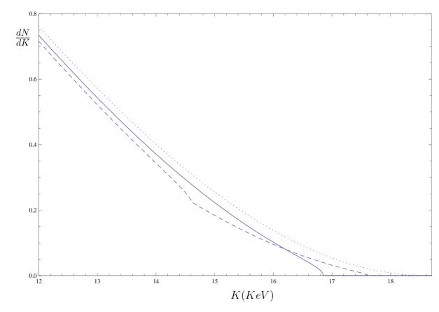
Figure 1: The tail of the tritium $\beta$ spectrum for: - a massless neutrino (dotted line); - fundamental flavor states (continuous line); - superposed prediction for 2 mass states (short-dashed line): notice the inflexion in the spectrum where the most massive state switches off. We used $m_{e}=1.75$ KeV, $m_{1}=1$ KeV, $m_{2}=4$ KeV, $\theta=\pi/6$.

If on the other hand we take flavor neutrinos as fundamental according to the above scheme, we have that $m_{\nu}=m_{e}$ and $K_{max}=Q-m_{e}$ and the spectrum is proportional to the phase volume factor $EpE_{e}p_{e}$:

$$\frac{dN}{dK}=CEp\,(Q-K)\sqrt{(Q-K)^{2}\,-\,m_{e}^{2}}\;\Theta(E_{e}-m_{e}).$$ (65)

The above discussed possibilities are plotted in Fig.(1), together with the spectrum for a massless neutrino, for comparison. We note that the next generation tritium beta decay experiments will allow a sub-eV sensitivity for the electron neutrino mass katrin , thus hopefully allowing to unveil the true nature of mixed neutrinos.

Finally we point out that also in the neutrino detection process, it would be possible to discriminate among the various scenarios above considered. In such a case, our scheme would imply that in each detection vertex, either an electron neutrino or a muon neutrino would take part to the process. Again, this is in contrast with the standard view, which assumes that either $\nu_{1}$ or $\nu_{2}$ are entering in the elementary processes.

V Discussion and Conclusions

In this paper we have studied a non-abelian gauge structure associated to flavor mixing. In this framework flavor neutrino fields are taken to be on-shell fields with definite masses $m_{e}$ and $m_{\mu}$, which are different from those of the mass eigenstates of the standard approach, $m_{1}$ and $m_{2}$. Flavor oscillations then arise as a consequence of the interaction with the gauge field, which acts as a sort of refractive medium – neutrino aether.

It would be interesting to explore the properties of such a medium and possible optical analogs of this situation. A very interesting example in this respect has been given recently in Ref.Weinheimer:2010ar . Another interesting analogy can be drawn with recent studies in which, for the case of photons, the vacuum has been thought to act as a refractive medium in consequence of quantum gravity fluctuations Ellis:2008gg .

The gauge structure associated to flavor mixing has the very interesting property of arising across different fermion generations, thus having a different (“horizontal”) nature with respect the gauge structure of the Standard Model.

A natural question that comes in concerns the origin of the external gauge field which causes the mixing. This could also have some connection to quantum gravity models that sometimes are invoked to explain the origin of mixing Mavromatos:2006ux .

Another outcome of our analysis is that we could recover, at least locally in time, a Poincaré structure for the flavor states. This is possible since we could define a Hamiltonian operator that commutes with the flavor charges, thus allowing for simultaneous eigenstates. In this scheme where the fields $\nu_{e}$ and $\nu_{\mu}$ are taken to be fundamental, one avoids any reference to the fields $\nu_{1}$ and $\nu_{2}$. As pointed out, this leads to phenomenological consequences that can be possibly tested in experiments on beta decay.

A final consideration concerns the interpretation of the Hamiltonian operator $\widetilde{H}$ which, as already remarked, does not take into account the interaction energy, i.e. the energy associated with mixing. We can thus view $\widetilde{H}$ as the sum of the kinetic energies of the flavor neutrinos, or equivalently as the energy which can be extracted from flavored neutrinos by scattering processes, the mixing energy being “frozen” (there’s no way to turn off the mixing!). This suggests the interpretation of such a quantity as a “free” energy $F\equiv\widetilde{H}$, so that we can write:

$$H-F=TS.$$ (66)

This quantity defines an entropy associated with flavor mixing. It is natural to identify the “temperature” $T$ with the coupling constant $g=\tan 2\theta$, thus leading to:

$$S = \int d^{3}\mathbf{x}\,{\bar{\nu}}_{f}A_{0}\nu_{f}\,=\,\frac{1}{2}\,\delta m\int d^{3}\mathbf{x}\,({\bar{\nu}}_{e}\nu_{\mu}+{\bar{\nu}}_{\mu}\nu_{e}).$$ (67)

The appearance of an entropy should not be surprising, since each of the two flavor neutrinos can be considered as an open system which presents some kind of (cyclic) dissipation. This situation can be handled by use of well known methods of Thermo Field Dynamics Umezawa:1982nv developed for the study of quantum dissipative systems CRV92 .

The explicit expression for the expectation values of the entropy on the flavor neutrino states is quite complicated, and thus not very illuminating. An attempt at an interpretation of it is given in Appendix B in the much simpler context of Quantum Mechanics. There it is shown that at a given time, the difference of the expectation values of the muon and electron free energies is less than the total initial energy of the flavor neutrino state. The missing part is proportional to the expectation value of the entropy.

The scenario emerged in this work, and in particular the last considerations, is consistent with an interpretation of the gauge field as a reservoir, first put forward in Celeghini:1992ea .

Finally, we point out that recent work Blasone:2007wp ; Blasone:2007vw ; Blasone:2010ta has shown that a time dependent entanglement entropy is associated with neutrino mixing and oscillations. It is an interesting question the one of the connection of the latter to the above entropy.

Appendix A Mixing of quantum neutrino fields

In this appendix we briefly recall the quantization for mixed fields, as given in Refs.BV95 ; BHV98 ; BJV01 . We start from the free fields $\nu_{1}$ and $\nu_{2}$, whose Fourier expansions are:

$$\nu_{j}(x)=\int\frac{d^{3}\mathbf{k}}{(2\pi)^{3/2}}\sum_{r}\left[u^{r}_{\mathbf{k},j}(x_{0})\alpha^{r}_{\mathbf{k},j}+v^{r}_{-\mathbf{k},j}(x_{0})\beta^{r\dagger}_{\mathbf{-k},j}\right]e^{i\mathbf{k}\cdot\mathbf{x}},\qquad j=1,2,$$ (68)

with $u^{r}_{\mathbf{k},j}(x_{0})=u^{r}_{\mathbf{k},j}e^{-i\omega_{\mathbf{k},j}x_{0}}$, $v^{r}_{-\mathbf{k},j}(x_{0})=v^{r}_{-\mathbf{k},j}e^{i\omega_{\mathbf{k},j}x_{0}}$, and $\omega_{\mathbf{k},j}=\sqrt{\mathbf{k}^{2}+m_{j}^{2}}$. The operators $\alpha^{r}_{\mathbf{k},j}$ and $\beta^{r}_{\mathbf{-k},j}$, $j=1,2$, $r=1,2$ are the annihilation operators for the vacuum state $|0\rangle_{1,2}=|0\rangle_{1}\otimes|0\rangle_{2}$: $\alpha^{r}_{\mathbf{k},j}|0\rangle_{1,2},\beta^{r}_{\mathbf{-k},j}|0\rangle_{1,2}=0$. The canonical anticommutation relations are: $\{\nu_{i}^{\alpha}(x),\nu_{j}^{\beta\dagger}(y)\}_{x_{0}=y_{0}}=\delta^{3}(\mathbf{x}-\mathbf{y})\delta_{\alpha\beta}\delta_{ij}$ with $\alpha,\beta=1,\ldots,4$ and $\{\alpha^{r}_{\mathbf{k},i},\alpha^{s\dagger}_{\mathbf{q},j}\}=\delta_{\mathbf{k}\mathbf{q}}\delta_{rs}\delta_{ij}$; $\{\beta^{r}_{\mathbf{k},i},\beta^{s\dagger}_{\mathbf{q},j}\}=\delta_{\mathbf{k}\mathbf{q}}\delta_{rs}\delta_{ij}$, with $i,j=1,2$. All other anticommutators are zero. The ortonormality and completeness relations are: $u_{{\bf k},j}^{r\dagger}u_{{\bf k},j}^{s}=v_{{\bf k},j}^{r\dagger}v_{{\bf k},j}^{s}=\delta_{rs}$, $u_{{\bf k},j}^{r\dagger}v_{-{\bf k},j}^{s}=v_{-{\bf k},j}^{r\dagger}u_{{\bf k},j}^{s}=0$, $\sum_{r}(u_{{\bf k},j}^{r}u_{{\bf k},j}^{r\dagger}+v_{-{\bf k},j}^{r}v_{-{\bf k},j}^{r\dagger})=1$.

We construct the generator for the mixing transformations (2) as:

$$\nu^{\alpha}_{\sigma}(x) = G_{\theta}^{-1}(x_{0})\nu^{\alpha}_{j}G_{\theta}(x_{0})\,,\qquad(\sigma,j)=(e,1),(\mu,2),$$ (69)

with $G_{\theta}(x_{0})$ given by:

$$G_{\theta}(x_{0})=\exp\left[\theta\int d^{3}\mathbf{x}\left(\nu_{1}^{\dagger}(x)\nu_{2}(x)-\nu_{2}^{\dagger}(x)\nu_{1}(x)\right)\right],$$ (70)

At finite volume $G_{\theta}$ is a unitary operator: $G_{\theta}^{-1}(x_{0})=G_{-\theta}(x_{0})=G_{\theta}^{\dagger}(x_{0})$, preserving the canonical anticommutation relations. $G_{\theta}^{-1}(x_{0})$ maps the Hilbert space for the free fields $\mathcal{H}_{1,2}$ to the Hilbert space for the mixed fields $\mathcal{H}_{e,\mu}$: $G_{\theta}^{-1}(x_{0}):\mathcal{H}_{1,2}\rightarrow\mathcal{H}_{e,\mu}$. In particular for the vacuum $|0\rangle_{1,2}$ we have, at finite volume $V$:

$$|0(x_{0})\rangle_{e,\mu}=G^{-1}_{\bf\theta}(x_{0})\;|0\rangle_{1,2}\;;$$ (71)

$|0\rangle_{e,\mu}$ is the vacuum for the Hilbert space $\mathcal{H}_{e,\mu}$, which we will refer us to as the flavor vacuum.

In the limit $V\rightarrow\infty$ the flavor vacuum becomes orthogonal to the vacuum of the free fields, which means that the two Hilbert spaces are unitarily inequivalent. Due to the linearity of $G_{\theta}(x_{0})$, we can define the flavor annihilators as:

$$\alpha_{{\bf k},\sigma}^{r}(x_{0}) \equiv G^{-1}_{\bf\theta}(x_{0})\;\alpha_{{\bf k},j}^{r}\;G_{\bf\theta}(x_{0}),\qquad(\sigma,j)=(e,1),(\mu,2)$$ (72)

and similar ones for the antiparticle operators. In the reference frame for which $\mathbf{k}=(0,0,|\mathbf{k}|)$, the electron neutrino annihilation operator has the form:

$$\alpha^{r}_{{\bf k},e}(x_{0}) = \cos\theta\;\alpha^{r}_{{\bf k},1}\;+\;\sin\theta\;\left(U_{{\bf k}}(x_{0})\;\alpha^{r}_{{\bf k},2}\;+\;\epsilon^{r}\;V_{{\bf k}}(x_{0})\;\beta^{r{\dagger}}_{-{\bf k},2}\right),$$ (73)

and similar expressions hold for the other ladder operators BV95 . Here $\epsilon^{r}=(-1)^{r}$ and:

$$U_{{\bf k}}(x_{0}) \equiv u^{r{\dagger}}_{{\bf k},2}(x_{0})u^{r}_{{\bf k},1}(x_{0})=v^{r{\dagger}}_{-{\bf k},1}(x_{0})v^{r}_{-{\bf k},2}(x_{0});$$ (74)

$$V_{{\bf k}}(x_{0}) \equiv \epsilon^{r}\;u^{r{\dagger}}_{{\bf k},1}(x_{0})v^{r}_{-{\bf k},2}(x_{0})=-\epsilon^{r}\;u^{r{\dagger}}_{{\bf k},2}(x_{0})v^{r}_{-{\bf k},1}(x_{0}),$$ (75)

and we have $U_{k}(x_{0})=|U_{k}|\;e^{i(\omega_{k,2}-\omega_{k,1})x_{0}}\;,V_{k}(x_{0})=|V_{k}|\;e^{i(\omega_{k,2}+\omega_{k,1})x_{0}}$, with $|U_{k}|^{2}\;+\;|V_{k}|^{2}\;=\;1$.

The flavor fields are then rewritten in the form:

$$\nu_{\sigma}(x)=\int\frac{d^{3}\mathbf{k}}{(2\pi)^{3/2}}\sum_{r}\left[u^{r}_{\mathbf{k},j}(x_{0})\alpha^{r}_{\mathbf{k},\sigma}(x_{0})+v^{r}_{-\mathbf{k},j}(x_{0})\beta^{r\dagger}_{\mathbf{-k},\sigma}(x_{0})\right]e^{i\mathbf{k}\cdot\mathbf{x}},\qquad(\sigma,j)=(e,1),(\mu,2),$$ (76)

i.e. they can be expanded in the same bases as the fields $\nu_{i}$.

The symmetry properties of the Lagrangian (1) have been studied in Ref. BJV01 : one has a total conserved charge $Q$ associated with the global $U(1)$ symmetry and time-dependent charges associated to the (broken) $SU(2)$ symmetry. Such charges are the relevant physical quantities for the study of flavor oscillations. They are also essential in the definition of physical flavor neutrino states, as the one produced in beta decay, for example.

We obtain for the flavor charges Eq.(9) the expansion BJV01 :

$$Q_{\sigma}(x_{0}) = \sum_{r}\int d^{3}\mathbf{k}\left(\alpha^{r\dagger}_{\mathbf{k},\sigma}(x_{0})\alpha^{r}_{\mathbf{k},\sigma}(x_{0})-\beta^{r\dagger}_{-\mathbf{k},\sigma}(x_{0})\beta^{r}_{-\mathbf{k},\sigma}(x_{0})\right).$$ (77)

Flavor neutrino states are defined as eigenstates of the flavor charges:

$$Q_{\sigma}(x_{0})|\nu_{\sigma}^{\mathbf{k}}(x_{0})\rangle = |\nu_{\sigma}^{\mathbf{k}}(x_{0})\rangle,$$ (78)

with $|\nu_{\sigma}^{\mathbf{k}}(x_{0})\rangle=\alpha^{r\dagger}_{\mathbf{k},\sigma}(x_{0})|0(x_{0})\rangle_{e,\mu}$, and similar ones for antiparticles.

Note that the flavor charges do not commute with the Hamiltonian of the system:

$$[H,Q_{\sigma}(x_{0})]\neq 0,\qquad\sigma=e,\mu$$ (79)

with the consequence that they are not conserved by time evolution. This of course gives rise to the oscillation phenomenon. The Hamiltonian and the flavor charges are thus non compatible observables, with the consequence that one cannot measure simultaneously the total energy and the flavor of an oscillating neutrino. The flavor states are however eigenstates of the momentum operator Eq. (7):

$$\mathbf{P}|\nu_{\sigma}^{\mathbf{k}}(x_{0})\rangle = \mathbf{k}|\nu_{\sigma}^{\mathbf{k}}(x_{0})\rangle.$$

The flavor oscillation formulas are derived by computing, in the Heisenberg representation, the expectation value of the flavor charge operators on the flavor state. We have

$${}_{e,\mu}\langle 0|:\;\!\!\;\!\!:Q_{\sigma}(x_{0}):\;\!\!\;\!\!:|0\rangle_{e,\mu}=0,$$ (80)

where $::...::\,$ denotes normal ordering with respect to the vacuum $|0\rangle_{e,\mu}$, defined in the usual way as $::A::\,\equiv\,A\,-\,{}_{e,\mu}\langle 0|A|0\rangle_{e,\mu}\$ for a generic operator $A$. The result is BHV98 :

$${\cal Q}^{\bf k}_{{\nu_{e}}\rightarrow\nu_{e}}(x_{0}) = \langle\nu_{{\bf k},e}^{r}|:\;\!\!\;\!\!:Q_{e}(x_{0}):\;\!\!\;\!\!:|\nu_{{\bf k},e}^{r}\rangle$$ (81)

$$= 1-\sin^{2}(2\theta)\left[\left|U_{\mathbf{k}}\right|^{2}\sin^{2}\left(\frac{\omega_{k,2}-\omega_{k,1}}{2}x_{0}\right)+\left|V_{\mathbf{k}}\right|^{2}\sin^{2}\left(\frac{\omega_{k,2}+\omega_{k,1}}{2}x_{0}\right)\right],$$

$${\cal Q}^{\bf k}_{{\nu_{e}}\rightarrow\nu_{\mu}}(x_{0}) = \langle\nu_{{\bf k},e}^{r}|:\;\!\!\;\!\!:Q_{\mu}(x_{0}):\;\!\!\;\!\!:|\nu_{{\bf k},e}^{r}\rangle\,=\,1\,-\,{\cal Q}^{\bf k}_{{\nu_{e}}\rightarrow\nu_{e}}(x_{0}).$$ (82)

In the relativistic limit: $\left|\mathbf{k}\right|\gg\sqrt{m_{1}m_{2}}$, we have $\left|U_{\mathbf{k}}\right|^{2}\longrightarrow 1$ and $\left|V_{\mathbf{k}}\right|^{2}\longrightarrow 0$ and the traditional oscillation formulas are recovered.

Appendix B The case of Quantum Mechanics

In this appendix we develop a similar analysis to the one given in this paper to the case of mixing in Quantum Mechanics. This is useful for the interpretation of the results, which in this case have a much simpler form.

In a QM context, the flavor (fermionic) annihilation operators are defined by the relations:

$$\alpha_{e}(t) = \cos\theta\,\alpha_{1}(t)+\sin\theta\,\alpha_{2}(t)$$ (83)

$$\alpha_{\mu}(t) = -\sin\theta\,\alpha_{1}(t)+\cos\theta\,\alpha_{2}(t),$$ (84)

where $\alpha_{i}(t)=e^{i\omega_{i}t}\alpha_{i}$, $i=1,2$. The flavor states are given by:

$$|\nu_{\sigma}(t)\rangle=\alpha^{\dagger}_{\sigma}(t)|0\rangle_{m},\qquad\sigma=e,\mu,$$ (85)

where $|0\rangle_{m}=|0\rangle_{1}\otimes|0\rangle_{2}$ is the vacuum for the mass eigenstates. We use the notation $|\nu_{\sigma}\rangle=|\nu_{\sigma}(t=0)\rangle$. The Hamiltonian of the system is:

$$H = \omega_{e}\alpha_{e}^{\dagger}(t)\alpha_{e}(t)+\omega_{\mu}\alpha_{\mu}^{\dagger}(t)\alpha_{\mu}(t)+\omega_{e\mu}\left[\alpha_{e}^{\dagger}(t)\alpha_{\mu}(t)+\alpha_{\mu}^{\dagger}(t)\alpha_{e}(t)\right]$$ (86)

$$= \omega_{1}\alpha_{1}^{\dagger}\alpha_{1}+\omega_{2}\alpha_{2}^{\dagger}\alpha_{2},$$

where $\omega_{e}=\omega_{1}\cos^{2}\theta+\omega_{2}\sin^{2}\theta$, $\omega_{\mu}=\omega_{1}\sin^{2}\theta+\omega_{2}\cos^{2}\theta$, $\omega_{e\mu}=(\omega_{2}-\omega_{1})\sin\theta\cos\theta$.

In analogy with the QFT case we define the covariant derivative:

$$D_{t}=\frac{d}{dt}+igA=\frac{d}{dt}+i\omega_{e\mu}\sigma_{1},$$ (87)

where we have $\omega_{e\mu}=\frac{1}{2}\tan 2\theta\delta\omega$, $\delta\omega=\omega_{\mu}-\omega_{e}$, and we have defined $A:=\delta\omega\frac{\sigma_{1}}{2}$. Using this covariant derivative the equations of motion read:

$$D_{t}\,\alpha_{f}=-i\omega_{d}\,\alpha_{f},$$ (88)

where $\alpha_{f}=(\alpha_{e},\alpha_{\mu})^{T}$ and $\omega_{d}=\textrm{diag}(\omega_{e},\omega_{\mu})$. The Hamiltonian can then be written in the form:

$$H=\alpha_{f}^{\dagger}\omega_{d}\alpha_{f}+g\alpha_{f}^{\dagger}A\alpha_{f}.$$ (89)

The diagonal part of the above expression can be readily split into separate contributions for each flavor

$$\widetilde{H}(t)=\alpha_{f}^{\dagger}\omega_{d}\alpha_{f}=\omega_{e}\alpha_{e}^{\dagger}(t)\alpha_{e}(t)+\omega_{\mu}\alpha_{\mu}^{\dagger}(t)\alpha_{\mu}(t)=\widetilde{H}_{e}(t)+\widetilde{H}_{\mu}(t).$$ (90)

Note that expectation values of the flavor number operators on the single particle flavor neutrino states at time zero give the oscillation probabilities:

$$\langle\nu_{e}(0)|N_{e}(t)|\nu_{e}(0)\rangle = P_{\nu_{e}\rightarrow\nu_{e}}(t)=1-\sin^{2}2\theta\text{ }\sin^{2}\left(\frac{\omega_{2}-\omega_{1}}{2}t\right);$$ (91)

$$\langle\nu_{e}(0)|N_{\mu}(t)|\nu_{e}(0)\rangle = P_{\nu_{e}\rightarrow\nu_{\mu}}(t)=\sin^{2}2\theta\text{ }\sin^{2}\left(\frac{\omega_{2}-\omega_{1}}{2}t\right).$$ (92)

Thus we have:

$$\langle\nu_{e}(0)|\widetilde{H}_{e}(t)|\nu_{e}(0)\rangle = \omega_{e}P_{\nu_{e}\rightarrow\nu_{e}}(t);$$ (93)

$$\langle\nu_{e}(0)|\widetilde{H}_{\mu}(t)|\nu_{e}(0)\rangle = \omega_{\mu}P_{\nu_{e}\rightarrow\nu_{\mu}}(t).$$ (94)

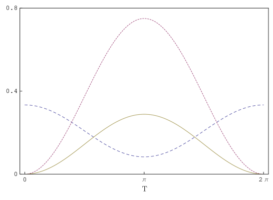
Figure 2: Plot of expectation values on $|\nu_{e}(0)\rangle$ of $F_{e}(t)$ (long-dashed line), $F_{\mu}(t)$ (short-dashed line) and $2TS_{e}(t)$ (solid line). We used rescaled dimensionless time $T=(\omega_{2}-\omega_{1})t$ and $\theta=\pi/6$. The scale on the vertical axis is normalized to $\omega_{\mu}$.

In analogy with the field theoretical case, we regard these “free” Hamiltonians as free energies, and we write:

$$H=\sum_{\sigma=e,\mu}(F_{\sigma}(t)+TS_{\sigma}(t)),$$ (95)

where we make the identifications $g\equiv T$ and:

$$S_{\sigma}(t)=\frac{1}{4}\;\delta\omega\left[\alpha_{e}^{\dagger}(t)\alpha_{\mu}(t)+\alpha_{\mu}^{\dagger}(t)\alpha_{e}(t)\right].$$ (96)

We have:

$$\langle\nu_{e}(0)|S_{e}(t)|\nu_{e}(0)\rangle=\langle\nu_{e}(0)|S_{\mu}(t)|\nu_{e}(0)\rangle=-\frac{1}{4}\;\delta\omega\sin 4\theta\sin^{2}\left[\frac{1}{2}(\omega_{2}-\omega_{1})t\right].$$ (97)

All the expectation values obtained are summarized in the following table, from which we immediately see how the energetic balance is recovered. The situation for an electron neutrino state is represented in Fig. 2 for sample values of the parameters.

	$H$	$F_{e}$	$F_{\mu}$	$TS_{e}=TS_{\mu}$
$|\nu_{e}(0)\rangle$	$\omega_{e}$	$\omega_{e}(1-P(t))$	$\omega_{\mu}P(t)$	$\frac{1}{2}\delta\omega P(t)$
$|\nu_{\mu}(0)\rangle$	$\omega_{\mu}$	$\omega_{\mu}P(t)$	$\omega_{e}(1-P(t))$	$-\frac{1}{2}\delta\omega P(t)$

Table 1: Energetic balance for flavor neutrino states. $P(t)$ denotes the transition probability $P_{\nu_{e}\rightarrow\nu_{\mu}}(t)$.

Note finally that the integral of the entropy expectation value over an oscillation cycle, is only dependent on the mixing angle:

$$\int_{0}^{\tau}\langle\nu_{e}(0)|S_{e}(t)|\nu_{e}(0)\rangle\,dt\,=\,\pi\cos^{2}2\theta\,\sin 2\theta.$$ (98)

where the period $\tau=\frac{2\pi}{\omega_{2}-\omega_{1}}$. It is interesting to compare this result with the geometric invariants discussed in Ref.Blasone:1999tq .

References

(1)
S. M. Bilenky and B. Pontecorvo,
Phys. Rept. 41 (1978) 225;
(2)
M. Blasone, A. Capolupo, F. Terranova and G. Vitiello,
Phys. Rev. D72 (2005) 013003;
(3)
C. C. Nishi,
Phys. Rev. D78 (2008) 113007;
(4)
M. Blasone and G. Vitiello,
Annals Phys. 244, 283 (1995);
(5)
K. Fujii, C. Habe and T. Yabuki Phys. Rev. D59,
113003 (1999); ibid. D64,
013011 (2001);
(6)
M. Binger and C. R. Ji,
Phys. Rev. D60 (1999) 056005;
C. R. Ji and Y. Mishchenko,
Phys. Rev. D64 (2001) 076004;
ibid. D65 (2002) 096015;
(7)
M. Blasone, A. Capolupo, O. Romei and G. Vitiello,
Phys. Rev. D63 (2001) 125015;
(8)
M. Blasone, A. Capolupo and G. Vitiello,
Phys. Rev. D66 (2002) 025033;
(9)
M. Blasone and J. Palmer,
Phys. Rev. D69 (2004) 057301;
(10)
M. Blasone, P.A. Henning and G. Vitiello,
Phys. Lett. B451, 140 (1999);
(11)
M. Blasone, P. P. Pacheco and H. W. Tseung,
Phys. Rev. D67 (2003) 073011;
(12)
M. Blasone, P. Jizba and G. Vitiello,
Phys. Lett. B517 (2001) 471;
(13)
M. Blasone, A. Capolupo, C. R. Ji and G. Vitiello,
[hep-ph/0611106];
(14) M. Blasone, J. Magueijo and P. Pires-Pacheco,
Europhys. Lett. 70 (2005) 600;
Braz. J. Phys. 35 (2005) 447;
(15)
J. Magueijo and L. Smolin,
Phys. Rev. D67 (2003) 044017;
Phys. Rev. Lett. 88 (2002) 190403;
(16)
C. Giunti,
Am. J. Phys. 72 (2004) 699;
M. Blasone, M. Di Mauro and G. Lambiase,
Acta Phys. Polon. B36 (2005) 3255;
(17)
S. Pakvasa,
[hep-ph/0110175];
G. Lambiase,
Phys. Lett. B560 (2003) 1;
V. A. Kostelecky and M. Mewes,
Phys. Rev. D69 (2004) 016005;
ibid. D70 (2004) 031902;
F. R. Klinkhamer,
Int. J. Mod. Phys. A21 (2006) 161;
E. Di Grezia, S. Esposito and G. Salesi,
Mod. Phys. Lett. A21 (2006) 349;
D. Hooper, D. Morgan and E. Winstanley,
Phys. Rev. D72 (2005) 065009;
J. R. Ellis, N. Harries, A. Meregaglia, A. Rubbia and A. Sakharov,
Phys. Rev. D78 (2008) 033013;
J. S. Diaz, V. A. Kostelecky and M. Mewes,
Phys. Rev. D80 (2009) 076007;
(18)
G. Amelino-Camelia,
Nature Phys. 3 (2007) 81;
J. Alfaro, H. A. Morales-Tecotl and L. F. Urrutia,
Phys. Rev. Lett. 84 (2000) 2318;
G. Lambiase,
Mod. Phys. Lett. A18 (2003) 23;
(19)
N. E. Mavromatos and S. Sarkar,
New J. Phys. 10 (2008) 073009;
(20)
J. Leite Lopes,
Gauge Field Theories. An Introduction,
(Pergamon, 1981);
(21)
Y. Aharonov and D. Bohm,
Phys. Rev. 115 (1959) 485;
(22)
M. Blasone and G. Vitiello,
Phys. Rev. D60 (1999) 111302;
(23)
A. Osipowicz et al.(KATRIN Coaboration),
[hep-ex/0109033];
(24)
C. Weinheimer,
Prog. Part. Nucl. Phys., 64 (2010) 205;
(25)
J. R. Ellis, N. E. Mavromatos and D. V. Nanopoulos,
Phys. Lett. B665 (2008) 412;
G. Gubitosi, G. Genovese, G. Amelino-Camelia and A. Melchiorri,
arXiv:1003.0878 [gr-qc];
(26)
N. E. Mavromatos and S. Sarkar,
[hep-ph/0604081];
S. H. S. Alexander,
arXiv:0911.5156 [hep-ph];
(27)
H. Umezawa, H. Matsumoto and M. Tachiki,
Thermo Field Dynamics and Condensed States,
(North-Holland, 1982);
(28)
E. Celeghini, M. Rasetti and G. Vitiello,
Ann. Phys. 215 (1992) 156;
(29)
E. Celeghini, E. Graziano, G. Vitiello and K. Nakamura,
Phys. Lett. B285 (1992) 98;
(30)
M. Blasone, F. Dell’Anno, S. De Siena and F. Illuminati,
arXiv:1003.5486 [quant-ph];
(31)
M. Blasone, F. Dell’Anno, S. De Siena, M. Di Mauro and F. Illuminati,
Phys. Rev. D77 (2008) 096002;
(32)
M. Blasone, F. Dell’Anno, S. De Siena and F. Illuminati,
EPL, 85 (2009) 50002;
(33)
M. Blasone, P. A. Henning and G. Vitiello,
Phys. Lett. B 466, 262 (1999);