Transport properties of $\nu=1$ quantum Hall bilayers. Phenomenological description.

Abstract

We propose a phenomenological model that describes counterflow and drag experiments with quantum Hall bilayers in a $\nu_{T}=1$ state. We consider the system consisting of statistically distributed areas with local total filling factors $\nu_{T1}>1$ and $\nu_{T2}<1$. The excess or deficit of electrons in a given area results in an appearance of vortex excitations. The vortices in quantum Hall bilayers are charged. They are responsible for a decay of the exciton supercurrent, and, at the same time, contribute to the conductivity directly. The experimental temperature dependence of the counterflow and drive resistivities is described under accounting viscous forces applied to vortices that are the exponentially increase functions of the inverse temperature. The presence of defect areas where the interlayer phase coherence is destroyed completely can result in an essential negative longitudinal drag resistivity as well as in a counterflow Hall resistivity.

1 Introduction

Theoretical prediction on superfluidity of bound electron-hole pairs in electron-hole bilayers [1, 2, 3, 4] and, especially, in quantum Hall bilayers [5, 6, 7, 8, 9, 10, 11, 12, 13] has stimulated experimental study of the counterflow transport in such systems. In these experiments [14, 15, 16, 17, 18, 19] electrical current is passed through one layer in a given direction and returned to the source through the other layer in the opposite direction. The counterflow currents in the adjacent layers can be provided by excitons that consist of an electron belonging to one layer and a hole belonging to the other layer. One can expect that at low temperature the gas of such excitons becomes superfluid and the counterflow current may flow without dissipation.

In the counterflow experiments [14, 15, 16, 17, 18, 19] bilayer quantum Hall systems with the total filling factor $\nu_{T}=1$ are used. At such a filling the number of electrons in one layer coincides with the number of empty quantum states (holes) in the lowest Landau level in the other layer. At rather small interlayer distances [20] the ground state of such a system is the BCS-like state with electron-hole pairing. The pairing is caused by the Coulomb attraction. The BCS-like state can also be considered as a superfluid state of interlayer excitons.

In spite of expectation to reach at low temperature zero electrical resistance, counterflow experiments in quantum Hall bilayers give some other results. At all temperatures a finite longitudinal resistance is registered. It decreases exponentially under lowering of temperature, but it does not vanish completely. Moreover, the counterflow longitudinal resistivity $\rho_{xx}^{CF}$ is even higher than the longitudinal resistivity measured in the parallel current geometry $\rho_{xx}^{\parallel}$ (in which the electrical currents in the adjacent layers are equal in value and flow in the same direction).

The excitons cannot give a contribution into the conductivity in the parallel current geometry. Therefore, the parallel current conductivity $\sigma_{xx}^{\parallel}$ should be much smaller than the counterflow conductivity $\sigma_{xx}^{CF}$. The relation between the longitudinal resistivities is another one. At zero or small Hall conductivity the longitudinal resistivity is in inverse proportion with the longitudinal conductivity. But for the conductivity tensor with a large Hall component the longitudinal resistivity is in direct proportion with the longitudinal conductivity. The first case is realized for the counterflow geometry and $\rho_{xx}^{CF}\approx 1/\sigma_{xx}^{CF}$. The parallel current geometry corresponds to the second situation and $\rho_{xx}^{\parallel}\approx\sigma_{xx}^{\parallel}/(\sigma_{xy}^{\parallel})^{2}$.

Exciton superfluidity can be imperfect due to phase slips caused by motion of vortices across the flow. In that case the counterflow resistivity is nonzero and, in principle, it can be larger than the parallel current resistivity. The smallness of $\rho_{xx}^{\parallel}$ can be accounted, for instance, for a small density of carriers that contribute into $\sigma_{xx}^{\parallel}$.

The specifics of the exciton superfluidity in bilayer quantum Hall systems is that the vortices carry electrical charges. Such vortices not only bring to a decay of superflow, but also give a direct contribution into conductivity. As was argued in [21], due to such a two-fold role of vortices, the counterflow and parallel current longitudinal resistivities coincide with each other (in the absence of other essential factors that may contribute to the conductivity).

The role of vortices in transport behavior of quantum Hall bilayers was considered in Ref. [22]. The consideration [22] is based on the coherence network model [23]. In this model superfluid excitons flow in a network formed by narrow links, and the dissipation is caused by vortices that cross these links. In [22] the drag geometry experiments are analyzed. In this geometry [15, 16, 17, 18] the current flows through one layer and the resistivities are measured in both layers. The resistivities in the active (drive) layer $\rho_{\alpha\beta}^{drive}$ and in the passive (drag) layer $\rho_{\alpha\beta}^{drag}$ are connected with $\rho_{\alpha\beta}^{\parallel}$ and $\rho_{\alpha\beta}^{CF}$ by the relations $\rho_{\alpha\beta}^{drive}=(\rho_{\alpha\beta}^{\parallel}+\rho_{\alpha\beta}^{CF})/2$ and $\rho_{\alpha\beta}^{drag}=(\rho_{\alpha\beta}^{\parallel}-\rho_{\alpha\beta}^{CF})/2$, where $\rho_{\alpha\beta}^{\parallel}$ and $\rho_{\alpha\beta}^{CF}$ are the resistivities of the layer that is used as an active one in the drag geometry (in case of imbalanced bilayers $\rho_{\alpha\beta}^{\parallel}$ and $\rho_{\alpha\beta}^{CF}$ are different for different layers). The resistivities $\rho_{xx}^{drive}$ and $\rho_{xx}^{CF}$ demonstrate thermally activated behavior. The activation energy depends asymmetrically on the imbalance of electron densities of the layers [16, 17]. As was shown in [22] this behavior can be described under assumption that vortex mobilities are thermally activated quantities and their activation energies are different for different specie of vortices. The vortex configurations in strongly disordered quantum Hall bilayers were studied in [24]. It was shown that disorder should be rather strong to provide vortex proliferation.

The ideas of [21, 22, 23, 24] are important for the understanding of transport properties of quantum Hall bilayers. Nevertheless, the question requires further study because a number of essential features should be explained. First of all, in all experiments the drag resistivity $\rho_{xx}^{drag}$ is negative and the counterflow resistivity $\rho_{xx}^{CF}$ is larger than the parallel current resistivity $\rho_{xx}^{\parallel}$. Actually, it is one of key points because in case of perfect exciton superfluidity $\rho_{xx}^{drag}$ should be positive and equal to $\rho_{xx}^{drive}$. Then, the origin of the counterflow Hall resistivity remains unclear. Also, the absolute value of $\rho_{xx}^{CF}$ observed experimentally is quite large and one can think about additional factors (beside vortices) that increase $\rho_{xx}^{CF}$.

In this paper we present a model in which transport features of quantum Hall bilayers are accounted for a special influence of imperfectness. We assume that due to imperfectness the local total filling factor deviates from unity and in some area $\nu_{T}<1$, while in other areas $\nu_{T}>1$. In the areas of the first (second) type positive-charged (negative-charged) vortices emerge. Besides, we imply that in some defect areas the interlayer phase coherence is destroyed completely. Using the effective medium approach [25, 26, 27] we compute the effective longitudinal and Hall resistivities for the counterflow, parallel current and drag geometries. The results are in good agreement with the experiment.

2 Vortices in exciton superfluids in quantum Hall bilayers

There are four species of vortices in the system considered [8]. Below they are notated by the index $\kappa=1,2,3,4$. The wave functions $|\kappa\rangle$ for the states with a single vortex can be presented as

$$|1\rangle=\prod_{m=0}^{M}\left(uc_{m,1}^{+}+vc_{m+1,2}^{+}\right)|0\rangle,$$ (1)

$$|2\rangle=\prod_{m=0}^{M}\left(uc_{m+1,1}^{+}+vc_{m,2}^{+}\right)|0\rangle,$$ (2)

$$|3\rangle=c^{+}_{0,2}\prod_{m=0}^{M}\left(uc_{m,1}^{+}+vc_{m+1,2}^{+}\right)|0\rangle,$$ (3)

$$|4\rangle=c^{+}_{0,1}\prod_{m=0}^{M}\left(uc_{m+1,1}^{+}+vc_{m,2}^{+}\right)|0\rangle.$$ (4)

Here $c_{m,i}^{+}$ is the operator of creation for an electron in the layer $i$ in the state with definite angular momentum $m$: $\Psi_{m}(r,\theta)=r^{m}e^{-im\theta}\exp(-r^{2}/4\ell^{2})$, where $\theta$ is the polar angle counted according to the right-hand rule with respect to the magnetic field direction, and $\ell=\sqrt{\hbar c/eB}$ is the magnetic length. The $u$ and $v$ coefficients are $u=\sqrt{\nu}$ and $v=\sqrt{1-\nu}$, where $\nu=\nu_{1}$ is the filling factor for the layer 1, and $1-\nu=\nu_{2}$ is the filling factor for the layer 2, $\nu_{i}=2\pi\ell^{2}n_{e,i}$, and $n_{e,i}$ is the electron density in the layer $i$.

Each vortex is characterized by distinct values of its vorticity and electrical charge. The vortex charge $q_{\kappa}$ can be found from the corresponding wave function (1). One can see from (1) that the charge of a given vortex is fractional and is concentrated in a certain layer. We notate this layer by $i_{\kappa}$.

The vortex is a state with a clockwise circular electrical current in one layer and a counterclockwise current in the other layer. We use the convention that the vortex has the positive vorticity $\alpha_{\kappa}=+1$ if the electrical current associated with the vortex is a counterclockwise in the layer 1 and clockwise in the layer 2. The vortex parameters for each specie are given in Table 1.

Table 1: The vorticity $\alpha_{\kappa}$, the electrical charge $q_{\kappa}$ and the layer $i_{\kappa}$ where the charge is concentrated, for four species of vortices

$\kappa$	$\alpha_{\kappa}$	$q_{\kappa}$	$i_{\kappa}$
1	-1	$e(1-\nu)$	2
2	+1	$e\nu$	1
3	-1	$-e\nu$	2
4	+1	$-e(1-\nu)$	1

The vortices nucleate in pairs. The components of the pair have the opposite vorticities. In the absence of electron deficit or excess the vortices in the pair have the opposite electrical charges, as well. The Coulomb attraction results in an increase of the binding energy of the pair. Therefore, free vortices at $\nu_{T}=1$ emerge at temperatures higher than the Berezinskii-Kosterlits-Thouless (BKT) transition temperature

Deviation of the total filling factor from unity forces the appearance of charge excitations that are transformed into vortex pairs. In a given pair each vortex has the fractional charge, but the sum of the charges is integer. In areas with electron deficit an equal number of vortices $\kappa=1$ and 2 is nucleated, and equal number of vortices $\kappa=3$ and 4 emerge in areas with electron excess. In a given area the vortices have the same sign of charge and due to Coulomb repulsion the size of a bound vortex pair can be quite large.

The energy of the pair is

$$E=\pi\rho_{s}\ln\frac{r}{a}+\frac{e^{2}\nu(1-\nu)}{\varepsilon r},$$ (5)

where $\rho_{s}$ is the superfluid stiffness, $r$ is the distance between the vortices, and $a$ is the vortex core radius. The energy (5) is minimum at the distance $r_{b}={e^{2}\nu(1-\nu)}/{\pi\varepsilon\rho_{s}}$. The quantity $\gamma=r_{b}(2n_{v})^{-1/2}$ (where $n_{v}$ is the concentration for one specie of vortices) yields the ratio of the vortex pair size to the average distance between the vortices. One can expect that at $\gamma>1$ a plasma of free vortices of opposite vorticities instead of a gas of vortex pairs emerges. Using the mean field value of $\rho_{s}$ [8] one finds that the condition $\gamma=1$ corresponds to the critical vortex density $n_{v,c}\approx 0.05n_{0}$, where $n_{0}=1/2\pi\ell^{2}$ is the electron density of a completely filled Landau level. The critical density $n_{v,c}$ is proportional to $\rho_{s}^{2}$. It is known that the mean-field approximation overestimates the superfluid stiffness $\rho_{s}$: it does not take into account quantum and thermal excitations, and the interaction with impurities that reduce the superfluid stiffness (see, for instance, [28, 29, 30]). Therefore, the actual critical density can be considerable smaller.

3 The resistivity caused by vortex motion

Let us consider the forces that act on a vortex. The vortices are electrically charged and the electric and magnetic components of the Lorentz force are applied to them:

$${\bf F}_{L}=q_{\kappa}{\bf E}_{i_{\kappa}}+q_{\kappa}{\bf v}_{\kappa}\times{\bf B}/c,$$

where ${\bf E}_{i}$ is the electrical fields in the layer $i$ and ${\bf v}_{\kappa}$ is the vortex velocity.

Vortices carry the vorticity and in system with nonzero net current the Magnus force ${\bf F}_{M}$ emerges. This force can be obtained from the derivative of the electrical current energy with respect to the vortex position (see, for instance, [31]):

$${\bf F}_{M}=2\pi\alpha_{\kappa}\rho_{s}\nabla\varphi\times\hat{z}.$$

Here $\hat{z}$ is the unit vector directed along the magnetic field, and $\nabla\varphi$ is the gradient of the phase of the order parameter taken far from the vortex center. The net currents in the layers read as ${\bf j}_{s1}=-{\bf j}_{s2}=e\rho_{s}\nabla\varphi/\hbar$. The Magnus force does not depend on the vortex velocity, because in the case considered this force is proportional to the difference of the net currents ${\bf j}_{s1}-{\bf j}_{s2}$. This difference is the same in the lab reference frame and the reference frame connected with a moving vortex.

We should also take into account the viscous force ${\bf F}_{\eta}=-\eta_{\kappa}{\bf v}_{\kappa}$, where $\eta_{\kappa}$ is the viscosity parameter. In what follows we will imply the vortex motion is connected with thermally activated hops of vortices between pinning centers. Is this case temperature dependence of the viscosity parameters can be approximated as $\eta_{\kappa}\propto\exp(\Delta_{\kappa}/T)$

In the stationary state the resultant force applied to the vortex is equal to zero

$$2\pi\alpha_{\kappa}\rho_{s}\nabla\varphi\times\hat{z}-\eta_{\kappa}{\bf v}_{\kappa}+q_{\kappa}{\bf E}_{i_{\kappa}}+\frac{q_{\kappa}}{c}{\bf v}_{\kappa}\times{\bf B}=0.$$ (6)

Eq. (6) is fulfilled for each specie $\kappa$ with nonzero density.

The motion of vortices across the flow results in a decay of the phase gradient. The rate of decay is $\partial(\nabla\varphi)/\partial t=\sum_{\kappa}2\pi n_{\kappa}\alpha_{\kappa}{\bf v}_{\kappa}\times\hat{z}$, where $n_{\kappa}$ is the density of vortices of specie $\kappa$. Antiparallel electrical fields applied to the layers may compensate this decay. They increase the phase gradient at the rate $\partial(\nabla\varphi)/\partial t=(e/\hbar)({\bf E}_{1}-{\bf E}_{2})$. In the stationary state the following condition should be satisfied

$$\sum_{\kappa}2\pi n_{\kappa}\alpha_{\kappa}{\bf v}_{\kappa}\times\hat{z}+\frac{e}{\hbar}({\bf E}_{1}-{\bf E}_{2})=0.$$ (7)

Having the vortex density one solves Eqs. (6) and (7) and finds the contribution of excitons and direct contribution of vortices into conductivity. To compute the conductivity tensor one should also take into account the bare conductivity of Landau level.

In the BCS-like state each electron is distributed between two one-particle states with the same guiding center index and distinct layer indices. The system responds on the resultant electrical force ${\bf F}_{E}=-N_{e}(\nu_{1}e{\bf E}_{1}+\nu_{2}e{\bf E}_{2})$ ($N_{e}$ is the total number of electrons) in the same manner as a completely filled Landau level responds on electrical field. In the latter case the electron gas moves as a whole with the drift velocity ${\bf v}_{0}=c{\bf E}\times{\bf B}/B^{2}$. In case of the bilayer system the expression for the drift velocity contains the effective field ${\bf E}_{eff}=\nu_{1}{\bf E}_{1}+\nu_{2}{\bf E}_{2}$. The velocity ${\bf v}_{0}$ can be also found from the condition that the electrical and magnetic components of the Lorentz force applied to the whole system compensate each other, as it takes place for a completely filled Landau level with negligible small relaxation

$$\nu_{1}{\bf E}_{1}+\nu_{2}{\bf E}_{2}+\frac{1}{c}{\bf v}_{0}\times{\bf B}=0.$$ (8)

The motion of an electron gas with the velocity ${\bf v}_{0}$ yields the contribution into the electrical currents $\delta{\bf j}_{i}=-en_{0}\nu_{i}{\bf v}_{0}$.

Thus, the electrical currents in the layer read as

$${\bf j}_{1}=-\sigma_{0}\nu_{1}\left(\nu_{1}{\bf E}_{1}+\nu_{2}{\bf E}_{2}\right)\times\hat{z}$$ (9)

$$+\frac{e}{\hbar}\rho_{s}\nabla\varphi+q_{2}n_{2}{\bf v}_{2}+q_{4}n_{4}{\bf v}_{4},$$ (10)

$${\bf j}_{2}=-\sigma_{0}\nu_{2}\left(\nu_{1}{\bf E}_{1}+\nu_{2}{\bf E}_{2}\right)\times\hat{z}$$ (11)

$$-\frac{e}{\hbar}\rho_{s}\nabla\varphi+q_{1}n_{1}{\bf v}_{1}+q_{3}n_{3}{\bf v}_{3},$$ (12)

where $\sigma_{0}=e^{2}/2\pi\hbar$

Tuning the magnetic field one can always fulfill the condition $\nu_{T}=1$ in average. But due to structural defects the local $\nu_{T}$ can be larger than unity in some areas and smaller than unity in other areas. For simplicity, we consider the system with two statistically distributed areas of equal fraction with local $\nu_{T1}>1$ and $\nu_{T2}<1$ ($(\nu_{T1}+\nu_{T2})/2=1$). In these areas the vortex densities for certain $\kappa$ are nonzero: $n_{1}=n_{2}=n_{v}$ in $\nu_{T}<1$ areas, and $n_{3}=n_{4}=n_{v}$ in $\nu_{T}>1$ areas ($n_{v}=n_{0}(\nu_{T1}-1)=n_{0}(1-\nu_{T2})$).

We start from the analysis of transport properties of balanced bilayers ($\nu_{1}=\nu_{2}$). In this case the electrical charges of the vortices are equal in modulus. It is reasonable to assume that the viscosity coefficients are the same for all species of vortices ($\eta_{1}=\eta_{2}=\eta_{3}=\eta_{4}=\eta$).

Solving Eqs.(6) and (7) and substituting the solition into Eq. (9) we obtain

$${\bf j}_{+}=\frac{\sigma_{0}}{2}\Bigg{[}\frac{n_{v}}{n_{0}}\frac{\eta\beta}{\eta^{2}+\beta^{2}}{\bf E}_{+}$$ (13)

$$-\left(1\pm\frac{n_{v}}{n_{0}}\frac{\beta^{2}}{\eta^{2}+\beta^{2}}\right){\bf E}_{+}\times\hat{z}\Bigg{]},$$ (14)

$${\bf j}_{-}=\frac{\sigma_{0}}{2}\frac{n_{0}}{n_{v}}\left[\frac{\eta}{\beta}{\bf E}_{-}\pm\left(1-\frac{2n_{v}}{n_{0}}\right){\bf E}_{-}\times\hat{z}\right],$$ (15)

In (13) the upper(lower) sign corresponds to $\nu_{T}>1$ ($\nu_{T}<1$) areas. Here we introduce the notation $\beta=\pi\hbar n_{0}$, ${\bf j}_{\pm}={\bf j}_{1}\pm{\bf j}_{2}$ and ${\bf E}_{\pm}={\bf E}_{1}\pm{\bf E}_{2}$. The system considered is a two-component isotropic conducting medium. Each component is characterized by the parameters $\sigma_{s}^{+}=\sigma_{xx}^{+}$, $\sigma_{a}^{+}=\sigma_{xy}^{+}$ (the parallel current conductivities) and $\sigma_{s}^{-}=\sigma_{xx}^{-}$, $\sigma_{a}^{-}=\sigma_{xy}^{-}$ (the counterflow conductivities).

The exact expressions for the effective conductivities can be obtained by the method developed in [25, 26]. In case of equal fractions of the components the effective quantities read as

$$\langle\sigma_{xx}^{\pm}\rangle=\sqrt{\sigma_{s1}\sigma_{s2}}\left(1+\frac{(\sigma_{a1}-\sigma_{a1})^{2}}{(\sigma_{s1}+\sigma_{s2})^{2}}\right)^{1/2},$$ (16)

$$\langle\sigma_{xy}^{\pm}\rangle=\frac{\sigma_{a1}\sigma_{s2}+\sigma_{a2}\sigma_{s1}}{\sigma_{s1}+\sigma_{s2}}.$$ (17)

Here $\sigma_{s(a)n}$ stands for $\sigma_{s(a)n}^{+}$ in the expression for $\langle\sigma_{\alpha\beta}^{+}\rangle$ and for $\sigma_{s(a)n}^{-}$ in the expression for $\langle\sigma_{\alpha\beta}^{-}\rangle$, the index $n=1,2$ numerates the components.

Using Eqs. (13) and (16), we obtain

$$\langle\sigma_{xx}^{+}\rangle=\frac{\sigma_{0}}{2}\frac{n_{v}}{n_{0}}\frac{\beta}{\sqrt{\eta^{2}+\beta^{2}}},\quad\langle\sigma_{xy}^{+}\rangle=-\frac{\sigma_{0}}{2},$$ (18)

$$\langle\sigma_{xx}^{-}\rangle=\frac{\sigma_{0}}{2}\frac{n_{0}}{n_{v}}\frac{\sqrt{\eta^{2}+\beta^{2}\left(1-\frac{2n_{v}}{n_{0}}\right)^{2}}}{\beta},\ \langle\sigma_{xy}^{-}\rangle=0.$$ (19)

The effective parallel current and counterflow resistivities are obtained from (18),(19) by the operation of inversion of the conductivity tensor. We take into account that $n_{v}/n_{0}$ is the small parameter. In the leading order in $n_{v}/n_{0}$ the resistivities equal to

$$\rho^{\parallel}_{xx}\approx\rho^{CF}_{xx}\approx\frac{2}{\sigma_{0}}\frac{n_{v}}{n_{0}}\frac{\beta}{\sqrt{\eta^{2}+\beta^{2}}},$$ (20)

$$\rho^{\parallel}_{xy}\approx\frac{2}{\sigma_{0}},\quad\rho^{CF}_{xy}=0,$$ (21)

$$\rho^{drive}_{xx}\approx\frac{2}{\sigma_{0}}\frac{n_{v}}{n_{0}}\frac{\beta}{\sqrt{\eta^{2}+\beta^{2}}},\ \rho^{drag}_{xy}=\rho^{drive}_{xy}=\frac{1}{\sigma_{0}},$$ (22)

$$\rho^{drag}_{xx}\approx-\frac{2}{\sigma_{0}}\left(\frac{n_{v}}{n_{o}}\right)^{2}\frac{\beta^{3}}{(\eta^{2}+\beta^{2})^{3/2}}.$$ (23)

The negative sign of $\rho^{drag}_{xx}$ means that the induced drag voltage is opposite to the voltage drop in the drive layer. Note that our model predicts rather small $\rho^{drag}_{xx}$ - it is quadratic in the small parameter $n_{v}/n_{0}$.

One can see that for large viscosity $\eta\gg\beta$ the resistivities $\rho^{\parallel}_{xx}\approx\rho^{CF}_{xx}\approx\rho^{drive}_{xx}\propto\exp(-\Delta/T)$, in an qualitative agreement with the experiment. The Hall resistivities $\rho^{\parallel}_{xy}$, $\rho^{drag}_{xy}$ and $\rho^{drive}_{xy}$ are in the quantitative agreement with experimental data.

Let us now consider the case of imbalanced bilayers. In imbalanced systems the vortex charges differ not only in sign but in absolute value. The viscosity is caused by the interaction of vortices with the pinning centers, so one can assume that the corresponding activation energy depends on the vortex charge. According to Table 1, we introduce two viscocity parameters $\eta_{a}=\eta_{1}=\eta_{4}$ and $\eta_{b}=\eta_{2}=\eta_{3}$. For simplicity, we restrict the analysis to the case of large viscosities $\eta_{a},\eta_{b}\gg\beta$. In this case one can neglect the difference of $\sigma_{ik}$ in $\nu_{T}>1$ and $\nu_{T}<1$ areas. Then, the relations between the currents and the fields are found to be

$${\bf j}_{+}\approx\frac{\sigma_{0}}{2}\Bigg{[}\frac{n_{v}}{n_{0}}\frac{2\beta}{\eta_{a}+\eta_{b}}{\bf E}_{+}-{\bf E}_{+}\times\hat{z}$$ (24)

$$+\frac{\eta_{a}-\eta_{b}}{\eta_{a}+\eta_{b}}{\bf E}_{-}\times\hat{z}\Bigg{]},$$ (25)

$${\bf j}_{-}\approx\frac{\sigma_{0}}{2}\Bigg{[}\frac{n_{0}}{n_{v}}\frac{2\eta_{a}\eta_{b}}{\beta(\eta_{a}+\eta_{b})}{\bf E}_{-}-(\nu_{2}-\nu_{1})^{2}{\bf E}_{-}\times\hat{z}$$ (26)

$$+\frac{\eta_{a}-\eta_{b}}{\eta_{a}+\eta_{b}}{\bf E}_{+}\times\hat{z}\Bigg{]}.$$ (27)

The inverse relations in linear in $n_{v}/n_{0}$ order are

$${\bf E}_{1}\approx\frac{1}{\sigma_{0}}\left[\frac{n_{v}}{n_{0}}\frac{2\beta}{\eta_{b}}{\bf j}_{1}+{\bf j}_{1}\times\hat{z}+{\bf j}_{2}\times\hat{z}\right],$$ (28)

$${\bf E}_{2}\approx\frac{1}{\sigma_{0}}\left[\frac{n_{v}}{n_{0}}\frac{2\beta}{\eta_{a}}{\bf j}_{2}+{\bf j}_{2}\times\hat{z}+{\bf j}_{1}\times\hat{z}\right].$$ (29)

It follows from (28) that

$$\rho_{1,xx}^{CF}\approx\rho_{1,xx}^{drive}\approx\frac{1}{\sigma_{0}}\frac{n_{v}}{n_{0}}\frac{2\beta}{\eta_{b}},$$ (30)

$$\rho_{2,xx}^{CF}\approx\rho_{2,xx}^{drive}\approx\frac{1}{\sigma_{0}}\frac{n_{v}}{n_{0}}\frac{2\beta}{\eta_{a}},$$ (31)

$$\rho_{1,xy}^{drive}\approx\rho_{2,xy}^{drive}\approx\rho_{xy}^{drag}\approx{\sigma_{0}}^{-1},\quad$$ (32)

$$\rho_{1,xy}^{CF}=\rho_{2,xy}^{CF}=0,\quad\rho_{xx}^{drag}=0.$$ (33)

Here $\rho_{n,\alpha\beta}$ notifies the resistivity in $n$-th layer.

One can see that the longitudinal resistivities of different layers are determined by different viscosities. Therefore, the resistivities may demonstrate different temperature dependences. It was observed experimentally that the activation energy for the longitudinal resistivities is higher in the layer with larger electron concentration. It corresponds to the grows of $\Delta_{\kappa}$ under increase of the vortex charge $q_{\kappa}$.

In addition, we note that in the leading order the Hall resistivities (32) are not sensitive to the imbalance as it was seen in experiments.

4 Possible origin of longitudinal drag resistivity

We have shown that due to specific relation between the vortex charge and the filling factor $\nu$ the resistivities $\rho_{1,xx}^{\parallel}$ and $\rho_{1,xx}^{CF}$ are very close to each other. They almost cancelled each other in the expression for the longitudinal drag resistivity, and the latter quantity (see Eq. (20)) is very small, in difference with experimental data that show considerable negative resistivity.

It is important to note that in case of perfect exciton superfluidity the longitudinal drag resistivity should be positive and equal to the drive resistivity. Indeed, any normal conductivity channel contributes into $\sigma_{xx}^{\parallel}$, so the resistivity $\rho_{xx}^{\parallel}$ should be nonzero. In the counterflow geometry the normal channel is shunted by superfluid excitons and cannot result in nonzero $\rho_{xx}^{CF}$. It yields $\rho_{xx}^{drag}=\rho_{xx}^{drive}=\rho_{xx}^{\parallel}/2$

In case of slightly imperfect exciton superfluidity the situation might be the following. An additional normal conductivity channel (not connected with free vortices) increases both $\sigma_{xx}^{\parallel}$ and $\sigma_{xx}^{CF}$. It results in an increase of $\rho_{xx}^{\parallel}$, but in a decrease $\rho_{xx}^{CF}$, so, it gives positive $\rho_{xx}^{drag}$. In particular, bound vortex pairs (which are charged are carry zero vorticity) should work in this direction. Thus, the question on the origin of negative longitudinal drag remains open.

In this section we will show that the negative drag can be accounted for the presence of defect areas, where the interlayer phase coherence is suppressed completely. For simplicity, we consider the case of balanced bilayers.

On a qualitative level the impact of defect areas can be understood as follows. In these areas the counterflow and parallel current conductivities are equal each other and coincide (at least, approximately) with the conductivities of a single layer with the filling factor $\nu=1/2$. The longitudinal conductivity of a single layer $\sigma_{xx}^{single}$ is much smaller than the counterflow conductivity determined by the exciton channel, and in the counterflow geometry the defect areas work as a sort of an exclude volume. Thus, the effective conductivity $\sigma_{xx}^{CF}$ decreases and the effective resistivity $\rho_{xx}^{CF}$ increases. On the other hand, if the conductivity $\sigma_{xx}^{single}$ is of the same order as the conductivity determined by the direct contribution of charged vortices the defect areas have only a small impact on the resistivity $\rho_{xx}^{\parallel}$.

To describe the influence of defect areas quantitatively we use the approach developed in [26]. According to [26], in general case of unequal fractions of the components the effective longitudinal and Hall conductivities of a two-component systems are given by the expressions

$$\langle\sigma_{xx}^{\pm}\rangle=\frac{\sigma_{s1}\sigma_{s2}(1-\lambda^{2})f[p,\lambda]}{D},$$ (34)

$$\langle\sigma_{xy}^{\pm}\rangle=\sigma_{a1}-\frac{(\sigma_{a1}-\sigma_{a2})\sigma_{s1}\lambda(1-f^{2}[p,\lambda])}{D},$$ (35)

where

$$D=\lambda(1-f^{2}[p,\lambda])\sigma_{s1}+(f^{2}[p,\lambda]-\lambda^{2})\sigma_{s2},$$

$$\lambda=\frac{1}{4\sigma_{s1}\sigma_{s2}}\Bigg{[}\sqrt{(\sigma_{s1}+\sigma_{s2})^{2}+(\sigma_{a1}-\sigma_{a2})^{2}}$$ (36)

$$-\sqrt{(\sigma_{s1}-\sigma_{s2})^{2}+(\sigma_{a1}-\sigma_{a2})^{2}}\Bigg{]}^{2},$$ (37)

$p$ is the fraction of the component 1, and

$$f[p,\lambda]=-\left(\frac{1}{2}-p\right)(1-\lambda)$$ (38)

$$+\sqrt{\left(\frac{1}{2}-p\right)^{2}(1-\lambda)^{2}+\lambda}\ .$$ (39)

Eq. (34) was obtained by mapping of the system with nonzero $\sigma_{xy}$ to the system with zero Hall conductivity. The function $f[p,x]$ approximates the effective conductivity $\langle\sigma\rangle$ of an isotropic two-dimensional two-component system with zero Hall conductivity: $\langle\sigma\rangle=\sigma_{1}f[p,\sigma_{2}/\sigma_{1}]$, where $\sigma_{i}$ is the longitudinal conductivity of the $i$-th component, and $p$ is the fraction of the component 1. The explicit expression (38) was obtained in the random resistor network approach [27].

The three-component system can be reduced to the two-component one in the following way. The defect areas are considered as the component 1. The rest areas with imperfect exciton superfluidity are considered as the component 2 with the conductivity equal to the effective conductivity of the system considered in the previous section.

Expressing the conductivities in $\sigma_{0}$ units, we have

$${\sigma}_{s1}^{+}={\sigma}_{s1}^{-}=\frac{\sigma_{xx}^{single}}{\sigma_{0}}=\alpha_{1},\ {\sigma}_{a1}^{+}={\sigma}_{a1}^{-}\approx\frac{1}{2},$$ (40)

$$\sigma_{s2}^{+}=\frac{n_{v}}{n_{0}}\frac{\beta}{2\sqrt{\eta^{2}+\beta^{2}}}=\alpha_{2},\ {\sigma}_{a2}^{+}=\frac{1}{2}$$ (41)

$$\sigma_{s2}^{-}=\frac{1}{4\alpha_{2}},\ \sigma_{a2}^{-}=0$$ (42)

The model contains two conductivity parameters $\alpha_{1}$, $\alpha_{2}$ (normally, $\alpha_{2}\lesssim\alpha_{1}\ll 1$) and the parameter $p$ (the defect area fraction).

The resistivity tensor is obtained by inversion of the effective conductivity tensor. The effective resistivities depend on $p$. Typical dependences are shown in Fig. 1.

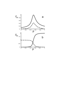
Figure 1: Longitudinal (a) and Hall resistivities (b) in units of $\sigma_{0}^{-1}$ versus the concentration of the areas with destroyed interlayer phase coherence. Solid curves - counterflow resistivities, dashed curves - drag resistivities. The longitudinal drag resistivity is given with reversed sign. The parameters $\alpha_{1}=0.05$ and $\alpha_{2}=0.025$ are used.

One can see that the longitudinal drag resistivity is nonzero (and negative). Other feature seen from Fig. 1 are the essential increase of the longitudinal and the appearance of Hall resistivity in the counterflow channel. The Hall drag resistivity is equal approximately to $\sigma_{0}^{-1}$ (that correspond to the experiment) if $p$ less and not to close to $1/2$.

5 Conclusion

Free vortices are dangerous for the superfluidity. But even in two-dimensional superfluid systems nucleation of vortices does not exclude perfect superfluidity. Below the BKT transition the vortices of opposite vorticities bind in pairs. Motion of such pairs, in difference with motion of single vortices, does not result in phase slips. The question is why it is not the case for quantum Hall bilayers.

In quantum Hall bilayers each elementary charge excitation produces two fractionally charged vortices that repulse due to Coulomb forces. There exists a critical charge excitation concentration above which a gas of unpaired vortices emerges. Due to renormalization of the superfluid stiffness the critical concentration can be rather small. If the condition $\nu_{T}=1$ is fulfilled in average and local total filling factor deviates from unity, the excess electrons or holes induce vortex excitations that suppress the superfluidity. If one trusts in the explanation presented one could expect that concrete values of counterflow, parallel current and drag resistivities are not universal quantities and may vary from sample to sample.

The problem of negative longitudinal drag resistivity forces to put forward the idea on the existence of areas with completely destructed interlayer coherence. This idea looks quite reasonable taking into account that real geometry of arms should result in essential edge effects (the presence of edge areas with destructed interlayer coherence). The same effect can be caused by structure defects and impurities in GaAs heterostuctures.

Nevertheless, one can hope that genuine exciton superfluidity can be realized in bilayer quantum Hall systems. The only problem that special requirements on purity and perfectness of the samples should be fulfilled.

References

- [1] S. I. Shevchenko, Sov. J. Low Temp. Phys. 2, 251 (1976); Phys. Rev. Lett. 72, 3242 (1994); Phys. Rev. B 56, 10355 (1997).
- [2] Yu. E. Lozovik, and V. I. Yudson, Sov. Phys. JETP 44, 389 (1976).
- [3] A. V. Balatsky, Y. N. Joglekar, P.B. Littlewood, Phys. Rev. Lett. 93, 266801 (2004); Y. N. Joglekar, A. V. Balatsky, M. P. Lilly Phys. Rev. B 72, 205313 (2005).
- [4] E. Babaev, Phys. Rev. B 77, 054512 (2008).
- [5] H. A. Fertig, Phys. Rev. B 40, 1087 (1989).
- [6] D. Yoshioka, A. H. MacDonald, J. Phys. Soc. Jpn. 59, 4211 (1990).
- [7] X. G. Wen and A. Zee, Phys. Rev. Lett. 69, 1811 (1992).
- [8] K. Moon, H. Mori, K. Yang, S. M. Girvin, A. H. MacDonald, L. Zheng, D. Yoshioka, and S. C. Zhang, Phys. Rev. B51, 5138 (1995).
- [9] S. M. Girvin, A. H. MacDonald, Multicomponent quantum hall systems: the sum of their parts and more Perspectives, in Quantum Hall Effects eds. S. D. Sarma and A. Pinczuk, New York: Wiley, 1997.
- [10] Yu. E. Lozovik and A. M. Ruvinsky, JETP 85, 979 (1997).
- [11] M. Abolfath, A. H. MacDonald, and L. Radzihovsky, Phys. Rev. B68, 155318 (2003).
- [12] A. I. Bezuglyj and S. I. Shevchenko, Phys. Rev. B 75, 75322 (2007).
- [13] S. H. Simon, Solid State Commun. 134, 81 (2005).
- [14] M. Kellogg, J. P. Eisenstein, L. N. Pfeiffer, and K. W. West, Phys. Rev. Lett. 93, 036801 (2004).
- [15] I. B. Spielman, M. Kellogg, J. P. Eisenstein, L. N. Pfeiffer, and K. W. West, Phys. Rev. B 70, 081303 (2004).
- [16] R. D. Wiersma, J. G. S. Lok, S. Kraus, W. Dietsche, K. von Klitzing, D. Schuh, M. Bichler, H.-P.Tranitz, and W. Wegscheider Phys. Rev. Lett. 93, 266805 (2004).
- [17] R. D. Wiersma, J. G. S. Lok, L. Tiemann, W. Dietsche, K. von Klitzing, D. Schuh, W. Wegscheider, Physica E 35, 320 (2006).
- [18] E. Tutuc, M. Shayegan, and D. A. Huse, Phys. Rev. Lett. 93, 036802 (2004).
- [19] E. Tutuc, M. Shayegan, Phys. Rev. B 72, 081307(R) (2005).
- [20] G. Moller, S. H. Simon, and E. H. Rezayi, Phys. Rev. B 79, 125106 (2009).
- [21] D. A. Huse, Phys. Rev. B 72, 064514 (2005).
- [22] B. Roostaei, K. J. Mullen, H. A. Fertig, S. H. Simon, Phys. Rev. Lett. 101, 046804 (2008).
- [23] H. A. Fertig, and G. Murthy, Phys. Rev. Lett. 95, 156802 (2005).
- [24] P. R. Eastham, N. R. Cooper and D. K. K. Lee, Phys. Rev. B 80, 045302 (2009).
- [25] A. M. Dykhne, Sov. Phys. JETP 32, 348 (1971).
- [26] D. Ya. Balagurov, Sov. Phys. JETP 81, 1200 (1995).
- [27] S. Kirkpatrick, Rev. Mod. Phys. 45, 574 (1973).
- [28] Y. N. Joglekar and A. H. MacDonald, Phys. Rev. B 64, 155315 (2001).
- [29] D. V. Fil, L. Yu. Kravchenko, Low Temp. Phys. 35, 712 (2009).
- [30] O. L. Berman, Yu. E. Lozovik, D. W. Snoke and R. D.Coalson, J. Phys.: Condens. Matter 19, 386219 (2007).
- [31] A. A. Abrikosov, Fundamentals of the Theory of Metals, North-Holland, Amsterdam, 1988.