The solar type protostar IRAS16293-2422: new constraints on the physical structure
Abstract
Context. The low mass protostar IRAS16293-2422 is a prototype Class 0 source with respect to the studies of the chemical structure during the initial phases of life of Solar type stars.
Aims. In order to derive an accurate chemical structure, a precise determination of the source physical structure is required. The scope of the present work is the derivation of the structure of IRAS16293-2422.
Methods. We have re-analyzed all available continuum data (single dish and interferometric, from millimeter to MIR) to derive accurate density and dust temperature profiles. Using ISO observations of water, we have also reconstructed the gas temperature profile.
Results. Our analysis shows that the envelope surrounding IRAS16293-2422 is well described by the Shu “inside-out” collapsing envelope model or a single power-law density profile with index equal to 1.8. In contrast to some previous studies, our analysis does not show evidence of a large ( AU in diameter) cavity.
Conclusions. Although IRAS16293-2422 is a multiple system composed by two or three objects, our reconstruction will be useful to derive the chemical structure of the large cold envelope surrounding these objects and the warm component, treated here as a single source, from single-dish observations of molecular emission.
Key Words.:
stars: formation – stars: individual: IRAS16293-2422 – ISM: molecules – ISM: abundances – stars: circumstellar matter – radiative transfer1 Introduction
Understanding how our Sun and Solar System formed is arguably one of the major goals of modern astrophysics. Many different approaches contribute to our understanding of the past history of the Solar System. Analyzing the relics of the ancient eons, comets and meteorites, is one. Studying present day objects similar to what the Sun progenitor is another. Here we pursuit the latter approach and analyze in detail the case of one of the best studied solar type protostars, IRAS16293-2422 (hereinafter IRAS16293). IRAS16293 is a Class 0 protostar in the Ophiuchus complex at 120 pc from the Sun (Loinard et al., 2008) and has played the role of a prototypical solar-type protostar for astrochemical studies, just as Orion KL has done for high-mass protostars. This is beause of its proximity and the resulting line strength of molecular emission (e.g. Walker et al., 1986; Mundy et al., 1992; Blake et al., 1994; van Dishoeck et al., 1995, to mention just a few representative works from the previous decades). It is in this source that the phenomenon of the “super-deuteration”111The super-deuteration refers to the exceptionally high abundance ratio of D-bearing molecules with respect to their H-bearing isotopologues found in low mass protostars, with observed D-molecule/H-molecule ratios reaching the unity (see e.g. the review in Ceccarelli et al., 2007). has been first discovered, with the detection of surprising abundant multiply deuterated molecules: formaldehyde, hydrogen sulfide, methanol and water (Ceccarelli et al., 1998; Vastel et al., 2003; Parise et al., 2003; Butner et al., 2007). It is also in this source that the first hot corino (Bottinelli et al., 2004; Ceccarelli et al., 2007) has been discovered, with the detection of several abundant complex organic molecules in the region where the dust grain mantles sublimate (Ceccarelli et al., 2000b; Cazaux et al., 2003; Bottinelli et al., 2004).
Not surprisingly, therefore, IRAS16293 has been the target of several studies to reconstruct its physical structure, namely the dust and gas density and temperature profiles (Ceccarelli et al., 2000a; Schöier et al., 2002, 2004; Jørgensen et al., 2005), the mandatory first step to correctly evaluate the abundance of molecular species across the envelope. Ceccarelli et al. (2000a) used water and oxygen lines observations obtained with the Infrared Space Observatory (ISO) to derive the gas and dust density and temperature profile. Conversely, Schöier et al. (2002) used the dust continuum observations to derive the structure of the envelope. Furthermore, while Ceccarelli et al. assumed the semi-analytical solution by Shu & co-workers (Shu, 1977; Adams & Shu, 1986) to fit the observational data, Schöier et al. (2002) assumed a single power law for the density distribution, and a posteriori verified that the Shu’s solution also reproduced the observational data. The two methods lead to similar general conclusions: a) the envelope of IRAS16293 is centrally peaked and with a density distribution in overall agreement with the inside-out collapse picture (Shu, 1977); b) there is a region, about 300 AU in diameter, where the dust mantles sublimate (giving rise to the phenomenon of the hot corino, mentioned above). However, the two different methods, not surprisingly, also lead to some notable differences. For example, the gas density differs by about a factor 3 in the region where the ice sublimation is predicted to occur, which leads to differences in the derived abundances of several molecular species.
Subsequent studies have built on the early ones to improve the derivation of the physical structure of IRAS16293. First, the study by Schöier et al. (2004), based on interferometric OVRO observations, concluded that the envelope has a large central cavity, about 800 AU in diameter. Then, the work by Jørgensen et al. (2005), using new SPITZER data, concluded that the envelope has an even larger central cavity, about 1200 AU in diameter. Such a large central cavity has a great impact on the whole interpretation of the hot corino of IRAS16293, as it predicts the absence of the mantle sublimation region. If the predicted cavity is real, the observed complex organic molecules must have another origin than grain mantle sublimation from thermally heated dust. In addition to rising an important point in itself, the Schöier and Jørgensen et al. works illustrate the paramount importance of correctly understanding the physical structure of the source to assess the chemical structure and all that follows.
For this reason, in the present work, we have re-analyzed the available data on IRAS16293 from scratch, considering, in addition, the most recent evaluation of the distance to this source by Loinard et al. (2008) (120 pc instead of 160 pc, as assumed in Ceccarelli et al., Schöier et al. and Jørgensen et al. works). This new analysis is necessary and timely because of two important observational projects having IRAS16293 as a target: a) the unbiased spectral survey in the 3, 2, 1 and 0.8 mm bands just obtained at the IRAM and JCMT telescopes (“The IRAS16293-2422 Millimeter And Sub-millimeter Spectral Survey”222http://www-laog.obs.ujf-grenoble.fr/heberges/timasss/; Caux et al., 2010, in prep.), and b) the unbiased spectral survey between 500 and 2000 GHz which will be obtained shortly with the heterodyne instrument HIFI aboard the Herschel Space Observatory (HSO) launched in May 2009 (the Herschel Guaranteed Time Key Program CHESS—Chemical Herschel Surveys of Star Forming Regions333http://www-laog.obs.ujf-grenoble.fr/heberges/chess/). The two projects, involving large international teams, will provide an accurate census of the molecular inventory of IRAS16293, the largest ever obtained in a solar type protostar. To convert the observations into an accurate chemical composition across the IRAS16293 envelope, the dust and gas density and temperature profiles have to be determined accurately first. Deriving these profiles is the goal of the present article.
We conclude this section by addressing the problem of the binarity of IRAS16293 and how it fits with the analysis we present here. As soon as interferometric observations became available it was realized that IRAS16293 is indeed a proto-binary system (Wootten, 1989; Mundy et al., 1992), composed by two sources: A (the south source) and B (the north source) separated by 4′′, i.e. 500 AU at 120 pc. While source B is the brightest in the continuum, source A is often, but not always, the brightest in the molecular emission (e.g. Chandler et al., 2005). The most recent observations show that IRAS16293 is indeed a triple system, with the source A composed by two objects, A1 and A2, of 0.5 and 1.5 M⊙ respectively (Loinard et al., 2009). While it is clear that the multiple nature of IRAS16293 cannot be neglected in general, the two projects mentioned above involve observations with single-dish telescopes, so that much of the structure on small scales is smeared out in these observations. Specifically, the molecular line emission will be dominated by the cold envelope, which fills up the telescope beam, and by any warm component at the interior of the envelope. The major goal here is to give a reliable estimate of the envelope temperature and density profiles of both the gas and dust components, up to the scales where the approximation of a spherical symmetry is valid. What are these scales will be discussed later on, based on the available observations.
The article is organized as follows. Section 2 discusses the derivation of the dust density and temperature distribution, based on the analysis of all available continuum data. Section 3 describes the derivation of the gas temperature profile, with the help of ISO data to constrain the abundance of a major gas coolant. Finally, Section 4 discusses and summarizes the results of the presented study.
2 Dust temperature and density profiles
2.1 The data set
The present analysis is based on the continuum emission from the
envelope that forms/surrounds the protostar IRAS16293. Three types of
observations are considered: maps of the emission, spectral energy
distribution (SED) and interferometric observations at 1 and 3 mm. All
data used have been retrieved from archives, except of the map at 350 m
and the 1 and 3 mm interferometric data that we obtained in dedicated
observations. Below we briefly describe the data used.
i) Continuum emission profiles
We used the maps of the dust continuum emission at 350 m (obtained at the Caltech Submillimeter Observatory; CSO), and 450 and 850 m (obtained at the James Clerk Maxwell Telescope; JCMT).
The 450 and 850 m maps have been retrieved from the JCMT archive (website). The beam sizes are 7.5′′ and 14.8′′ at 450 and 850 m respectively. Based on the many previous JCMT published observations, the calibration uncertainty and noise levels are 10% and 0.04 Jy beam-1 at 850 m and 30% and 0.3 Jy beam-1 at 450 m, respectively.
Observations of the 350 m continuum emission toward IRAS 16293 reported here were carried out in 2003 February using the SHARC II facility bolometer camera of the Caltech Submillimeter Observatory (CSO) on Mauna Kea in Hawaii (Dowell et al., 2003). SHARC II is a pixel filled array with a field of view of . The data were taken during excellent submillimeter weather conditions (a 225 GHz zenith opacity of 0.04, corresponding to less than 1 mm of precipitable water). The observations were carried out using the “box-scan” scanning mode (see http://www.submm.caltech.edu/sharc/). Five 10 min scans were reduced together using the CRUSH software package (Kovács, 2008) to produce the final calibrated image. Telescope pointing was checked on Juno, Vesta, or Mars, immediately before or after the science observations and the measured offsets were applied during data reduction. The data were taken before the CSO Dish Surface Optimization system (DSOS) become operational. The shape of the telescope beam was determined from the pointing images of Vesta and Mars. It contains a diffraction limited main beam with a FWHM diameter of 9′′ and an error beam with a FWHM diameter of 22′′, with relative peak intensities of 0.8 and 0.2, respectively. This size of the error beam is consistent with earlier 350 m measurements using the SHARC I camera (Hunter, 1997).
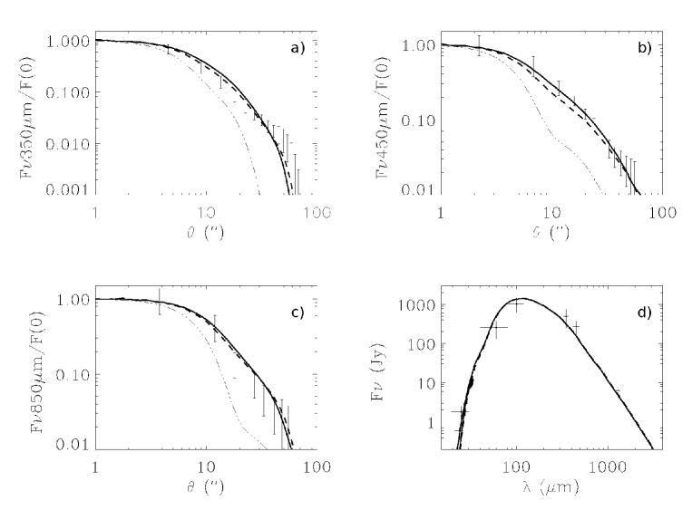
We obtained continuum emission profiles as function of the distance from the center of the envelope, by averaging the map emission over annuli at the same distance. In each case we adopted a radial sampling corresponding to the half of the resolution of the instrument. The uncertainties of continuum emission profiles were evaluated taking into account the calibration uncertainty, noise levels and the non sphericity of the source. The resulting profiles, normalized to the peak emission, are shown in Fig. 1. Note that the 450 and 850 m profiles are identical to those reported by Schöier et al. (2002).
ii) Spectral Energy Distribution
Table 1 reports the SED obtained considering all the data available in the literature (plus the 350 m point obtained by us; see above). The millimeter and sub-millimeter data points have been obtained by integrating the maps over the entire envelope. The integrated flux at 1.3 mm was that quoted in Saraceno et al. (1996). We retrieved the IRAS fluxes from the IRAS Point Source Catalog v2.1 (http://irsa.ipac.caltech.edu/cgi-bin/Gator/nph-dd?catalog=iraspsc).
| Fνa𝑎aa𝑎aIntegrated flux in Jy | Fνb𝑏bb𝑏bUncertainties in Jy considering the calibration uncertainty, the noise levels and the uncertainty on the source size. | c𝑐cc𝑐cMain beam of the instrument in arcsec. | Ref. | |
|---|---|---|---|---|
| (m) | (Jy) | (Jy) | (“) | |
| 23.7 | 0.6 | 0.1 | 6.0 | 2 |
| 25 | 1.8 | 0.7 | 80.0 | 3 |
| 60 | 255. | 122. | 160.0 | 3 |
| 100 | 1032. | 412. | 237.0 | 3 |
| 350 | 500. | 250. | 9.0 | 1 |
| 450 | 270. | 108. | 7.8 | 1 |
| 850 | 20.2 | 8. | 14.5 | 1 |
| 1300 | 6.4 | 2.6 | 22.0 | 4 |
$a$$a$footnotetext: Integrated flux in Jy. $b$$b$footnotetext: Uncertainties in Jy considering the calibration uncertainty, the noise levels and the uncertainty on the source size. $c$$c$footnotetext: Main beam of the instrument in arcsec.
(1) This paper; (2) Spitzer catalog; (3) IRAS Point Source Catalog v2.1; (4) Saraceno et al. (1996).
IRAS 16293 was observed with the InfraRed Spectrograph (IRS)
installed aboard the Spitzer Space Telescope as part of the
“From Molecular Cores to Planet Forming DIsks” (Evans et al., 2003; Evans & c2d Team, 2005) Legacy Program
(AOR: 11826944, PI: Neal Evans). We use the observations obtained with
the Long-High (LH) module (20-37 m, R 600) on
2004 July 29, in staring mode. The data reduction was performed using the
c2d
pipeline S15.3.0 (Lahuis et al., 2006) with the pre-reduced (BCD)
data. Since the MIPS map at 24 m shows that the IRAS16293
emitting region ( 30-40′′) is larger than the LH module field of
view (11.1′′ 22.3′′), we adopted the full aperture extraction
method in the pipeline. In addition, we corrected the derived flux
level for the missing flux by comparing the IRS spectrum integrated on
the MIPS bandwith and the integrated MIPS flux. Note that this method
assumes a similar distribution of the source emission in the whole
IRS wavelength interval, 21-37 m. The correction factor
derived by this method amounts to 22 in the flux.
iii) Interferometric continuum data
Observations of the 3 and 1.3 mm continuum were obtained with the IRAM Plateau de Bure Interferometer (PdBI) in 2004 and are described in detail in Bottinelli et al. (2004). They were obtained in B and C configurations of the PdBI array, resulting in a spatial resolution of about 0.8′′.
2.2 Adopted model
We obtained the best fit to the continuum data, described in the previous section, by using the 1D radiative transfer code DUSTY (Ivezic & Elitzur, 1997), which has been extensively used in similar works (including Jørgensen et al., 2002; Schöier et al., 2002, 2004; Jørgensen et al., 2005). Briefly, giving as input the temperature of the central object and a dust density profile, DUSTY self-consistently computes the dust temperature profile and the dust emission. A comparison between the computed 350, 450, 850 m brightness profiles (namely the brightness versus the distance from the center of the envelope) and SED with the observations (described in the previous section) allows to constrain the density profile and, consequently, the temperature profile of the envelope. To be compared with the observations, the theoretical emission is convolved with the beam pattern of the telescope. Following the recommendations for the relevant telescope, the beam is assumed to be a combination of Gaussian curves: at 850 m, we use HPBWs of 14.5′′, 60′′, and 120′′, with amplitudes of 0.976, 0.022, and 0.002 respectively; at 450 m, the HPBWs are 8′′, 30′′, and 120′′ with amplitude ratios of 0.934, 0.06, and 0.006, respectively (Sandell & Weintraub, 2001); at 350 m, we use HPBWs of 9′′ and 22′′, with amplitude ratios of 0.8, 0.2, respectively (Section 2.1).
In this work, we consider two cases for the density distribution. In the first one, we assum a broken power-law density profile as in the Shu (1977) solution:
| (1) |
| (2) |
where is the radius of the collapsing envelope (at larger radii the envelope is static). In the density profile, it represents the radius at which the change of index occurs and it is a free parameter. Note that the complete Shu (1977) solution also contains a transition part at the interface of the collapsing and static regions, just inside . In this region the slope gradually changes from r-1 to the limiting value of r-1.5. A posteriori, the effective part of the envelope in r-1 is relatively small and located in the inner region ( 1500 AU, equivalent to 10”). Since the continuum observations, with resolutions of 8-18, are not sensitive enough, we adopted the simplified structure described by the Eq. 1,2. In the second case, we considered a single power-law density profile, where the index is a free parameter:
| (3) |
In both cases, is the density at , and the envelope starts at a radius and extends up to . In total, both models have four free parameters determined by the best fit with the observational data: or , , and . Finally, DUSTY requires the temperature of the central source, T∗, here assumed to be 5000 K. Note that we verified that the choice of this parameter does not influence the results, as already noticed by other authors (e.g. Jørgensen et al., 2002). In practice, the DUSTY input parameters are the infall radius or the power-law index , the optical thickness at 100 m, , the ratio between the inner and outer radius, Y (=/) and the temperature at the inner radius Tin444The temperature at the inner radius Tin in fact defines the radius at which the integration starts. The DUSTY codes requires the temperature rather than the radius because it is based on a scale-free algorithm.. The optical thickness is, in turn, proportional to and . In both models, we obtain a lower limit to Tin of 300 K, any larger value giving similar results.
In addition to the above parameters, the opacity of the dust as function of the wavelength is a hidden parameter of DUSTY. Following numerous previous studies (Van Der Tak et al., 1999; Evans et al., 2001; Shirley et al., 2002; Young et al., 2003; Schöier et al., 2002), we adopted the dust opacity calculated by Ossenkopf & Henning (1994), specifically their OH5 dust model, which refers to grains coated by ice. Again, the basic result, though, does not substantially depend on the choice of the dust opacity model.
As explained in Ivezic & Elitzur (1997), DUSTY gives scale-free results, so that the source bolometric luminosity Lbol and the distance are required to compare the DUSTY output with actual observations. We assumed here the lastest estimate of the distance to the Ophiuchus cloud, namely 120 pc (see Introduction), and we derived the bolometric luminosity by integrating the observed emission over the full spectrum, optimizing the resulting (see below).
We run grids of models for both cases described above. The summary of the covered parameter space is reported in Table 2.
| Parameter | Range | Step |
|---|---|---|
| 0.2–2.5 | 0.1 | |
| Ya | 50–2000 | 10 |
| rinf | 5–200 | 2 |
| 0.1–10. | 0.1 | |
| Tin | 300 K | Fixed |
| T∗ | 5000 K | Fixed |
a Y = rout/rin
The best fit model has been found minimizing the with an iterated two-steps procedure (see also Crimier et al., 2009). First, we use the observed brightness profiles at 350, 450 and 850 m to constrain Y and (or rinf in the case of the Shu-like model), assuming a value for . Second, we constrain the optical thickness by comparing the computed and observed SED, assuming the (or rinf) and Y of the previous step. The new is used for a new iteration and so on. In practice, the iteration converges in two steps. This is because the normalized brightness profiles depend very weakly on , while they very much depend on the assumed size of the envelope and on the slope of the density profile (see also the discussion in Jørgensen et al., 2002; Crimier et al., 2009). In contrast, the dust optical thickness depends mostly on the absolute density of the envelope. Note that we constrain also the bolometric luminosity based on the best fit of the SED 555Note that the dust optical thickness affects the shape of the SED, so in general it enters in the determination of the bolometric luminosity..
2.3 Results
a) Brightness profiles and SED analysis
Table 3 lists the best fit parameters for the two models described in the previous section as well as the parameters obtained by Schöier et al. (2002) for comparison. Figure 1 shows the solutions compared to the observed data (maps and SED).
| Quantity | Shu-like model | Power-law model | Schöier et al. (2002) |
|---|---|---|---|
| L∗ (L⊙) | 22 | 22 | 27 |
| D (pc) | 120 | 120 | 160 |
| 2.0 | 3.0 | 4.5 | |
| (AU) | 1280 | ||
| 1.8 | 1.7 | ||
| Y | 280 | 260 | 250 |
| (AU) | 22 | 27 | 32 |
| (AU) | 6100 | 6900 | 8000 |
| r(Tdust=100K) (AU) | 76 | 85 | |
| n(Tdust=100K) (cm-3) | |||
| Menv (M⊙) | 1.9 | 2.1 | 5.4 |
The results of this part of the analysis are:
- •
-
•
The single power-law and Shu-like density distributions can both reproduce the observations, the maps and the SED data, included the IR part of the spectrum (Figure 1). They give similar best fit values, although the Shu-like distribution fits better the 450 m profile. Also the derived physical parameters are substantially similar for the two models.
-
•
The observed data, including the Spitzer data between 20 and 40 m, do not necessitate the presence of a large cavity (Jørgensen et al., 2005). Our solution with a larger luminosity (22 instead of 14 L⊙) can reproduce as well the MIR Spitzer observations. Figure 2 shows the MIR Spitzer and IRAS observations against the emission predicted by our models and these by Jørgensen et al. (2005) and Schöier et al. (2002).
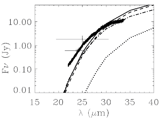
Figure 3 shows the derived dust temperature and density profiles. The single power-law index density distribution predicts a slightly warmer and denser region at radii lower than about 100 AU, but the differences are relatively small (see also Table 3).


b) Interferometric data analysis
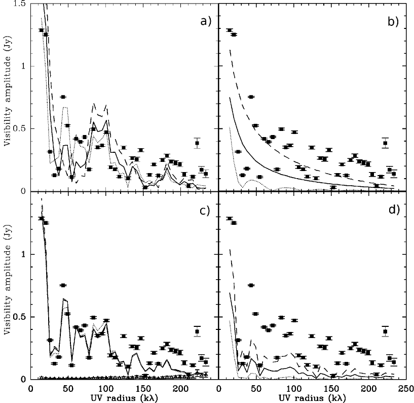
The previous analysis considers single dish data, which at best have a spatial resolution of 8′′, equivalent to a radius of AU. In order to constrain better the inner region, we used 1 and 3 mm continuum interferometric observations obtained with the Plateau de Bure interferometer (PdBI) described in the previous section. In order to compare the model predictions with the observations, we have produced synthetic maps for each model, in which we added the predicted emission from the envelope plus the emission of the two Gaussian-like sources A and B. The parameters used to represent the emission of the sources A and B are extracted from the interferometric maps at 1.3 and 3 mm and reported in Table 4. Then we used the UVFMODEL task in Gildas666http://iram.fr/IRAMFR/GILDAS/doc/html/mis-html/node13.html to compute visibility tables with the same uv plane coverage than the actual observations.
| 1.3mm | 3mm | |||
|---|---|---|---|---|
| Source | Fν(Jy) | FWHM(”) | Fν(Jy) | FWHM(”) |
| A | 0.49 | 1.18 | 0.16 | 1.62 |
| B | 0.97 | 0.86 | 0.25 | 0.78 |
Table 5 reports the values obtained using the observed and modeled visibility amplitudes at 1.3 mm. The comparison is done for each of the three models of the envelope, i.e. the single power-law density distribution, the Shu-like density distribution, and the central cavity of Schöier et al. (2004). We tested cases in which the envelope is centered on one of the two sources or on the mid-way point between the two sources. The values are computed over more than 104 points. The 2D representation of the visibility amplitudes observed and modeled in uv plan is difficult to read. Therefore to illustrate the comparison between the visibility amplitudes observed and modeled, we averaged the visibility amplitudes over the same uv radius and plotted them in Figure 4. Note that the error bars shown in Fig. 4 represent only the measurement errors. In fact, the standard deviations resulting from the radial average are meaningless in this case because of the non-sphericial geometry (caused by the presence of the sources A and B). Figure 4 only aims to illustrate the comparison between the observations and models, our conclusions will be based on the in Table 5. The computations were done considering all the visibility amplitudes obtained in the uv plane before the azimuthal average.
The interferometric data
are dominated by the two components of the IRAS16293 binary system. However, regarding
the envelope contribution—which is relevant for the present work—in
the case where the envelope is centered on the mid-way point between the sources A and
B, the visibilities at uv radii lower than about 80 k are not
well reproduced by the single power-law density profiles. Our solution
with the Shu-like density profile and the solution with a cavity
(suggested by Schöier et al. 2004) give a much better agreement. However, when envelope is centered on B or A
all three models give similar results (Fig. 4), and fit well
the observed visibilities. Since with the data available in the
literature there is no way to know whether the envelope is centered on
one of the two sources (A or B) or just on the mid-way point between them, either of the
two solutions (centered on a source or on the mid-way point
between A and B) is equally plausible. In other words, we
are in a degenerated case dominated by the parameters relative to
the binarity of the source. The interferometric data can be
reproduced without a cavity.
Note that the 3 mm PdBI observations do not provide additional information.
We emphasize that the above analysis of the interferometric data is
directly applicable to the OVRO data that led Schöier et al. (2004) to suggest
the presence of a cavity. The OVRO data probe visibility amplitudes
lower than about 60 k, a range also probed by the PDBI
data. Therefore, as shown above, they can be reproduced by assuming
that the envelope is centered on either A or B source without the
necessity of assuming a cavity.
| 1.3 mm | Model centered | Model centered | Model centered |
|---|---|---|---|
| in between A and B | on B | on A | |
| Model | |||
| Single power-law | 18.5 | 10.2 | 8.5 |
| Shu-like | 13.3 | 10.3 | 8.3 |
| Central cavity | 11.0 | 11.3 | 9.9 |
c) Summary of the continuum data analysis
Both the single dish and interferometric continuum data can be reproduced by either of the two models we considered: a Shu-like and single power-law density distribution. Furthermore, no cavity is required to explain the data, neither the Spitzer MIR data (Jørgensen et al., 2005) nor the interferometric data (Schöier et al., 2004).
Therefore, in the following we will adopt the Shu-like density profile (which has a physical interpretation), with no cavity, as our reference model for the study of the gas temperature and water line predictions.
3 Gas temperature profile
3.1 Adopted method
We computed the gas temperature profile using the CHT96 code described in Ceccarelli et al. (1996) (see also Ceccarelli et al., 2000a; Maret et al., 2002; Crimier et al., 2009). Briefly, the code computes the gas equilibrium temperature at each point of the envelope, by equating the heating and cooling terms at each point of the envelope. Following the method described in Ceccarelli et al. (1996), we considered heating from the gas compression (due to the collapse), dust-gas collisions and photo-pumping of H2O and CO molecules by the IR photons emitted by the warm dust close to the center777Cosmic rays ionization is a minor heating term in the protostellar envelopes.. The cooling terms are the line emission from H2O, CO and O. The dust-gas collisions are a source of heating when the dust temperature is higher than the gas temperature and a source of cooling elsewhere. To compute the cooling from the lines we used the code described in Ceccarelli et al. (1996, 2003) and Parise et al. (2005). The same code has been used in several past studies, whose results have been substantially confirmed by other groups (e.g. the analysis on IRAS16293-2422 by Schöier et al. 2002). Briefly, the code is based on the escape probability formalism in presence of warm dust (see Takahashi et al., 1983), where the escape probability is computed at each point by integrating the line and dust absorption over the solid angle as follows:
| (4) |
where and are the line and dust absorption coefficients respectively, and is the line trapping region, given by the following expressions:
| (5) |
in the infalling region of the envelope (where is the angle with the radial outward direction) and in the static region (where is the envelope radius):
| (6) |
In addition, H2O and CO molecules can be pumped by absorption of the NIR photons emitted by the innermost warm dust. Since the densities and temperatures of the regions of the envelope targeted by this study are not enough to populate the levels in the vibrational states, the effect of the NIR photons is an extra heating of the gas, as described in Ceccarelli et al. (1996). Note that the code takes into account the dust with temperatures up to 1500 K.
The code has a number of parameters, that influence the gas equilibrium temperature. First, the dust temperature, assumed to be the output of the previous step analysis (§2). Second, since the infall heating depends on the velocity gradient across the envelope and the cooling depends on the gas lines (which can and are sometimes optically thick), the velocity field across the envelope is also a parameter of the code. Here we assumed that the infall velocity field corresponds to the free fall velocity field with a 2 M⊙ source at the center of the envelope (Loinard et al., 2009). Third we adopted the “standard” cosmic rays ionization rate, namely s-1, however, in practcie this parameter is unimportant. Finally, given the contributions of the H2O, CO and OI to the gas cooling, their respective abundances are important parameters of the model. Previous theoretical studies have shown that the O abundance is constant across the envelope, except in the very inner regions, where the gas temperature exceeds about 250 K and endothermic reactions that form OH and H2O become very efficient (Ceccarelli et al., 1996; Doty & Neufeld, 1997; Doty et al., 2004). Unfortunately, this parameter is very poorly constrained by observations (because of the difficulty of observing the O fine structure lines and the fact that they are easily excited in the foreground molecular cloud and its associated PDR (see e.g. Liseau et al., 1999; Caux et al., 1999). Here we assumed that the atomic O abundance is equal to and verified a posteriori that the O fine structure line emission is consistent with the ISO observations. We note, however, that O is never the dominant coolant except, perhaps, in a very small region of the envelope (Ceccarelli et al., 2000a; Maret et al., 2002). CO, in contrast, is the main coolant in the outer envelope, but, since the cooling lines are heavily optically thick, its abundance does not play an important role (in the regime where it is higher than about with respect to H2). We, therefore, assumed a canonical CO abundance across the envelope.888Note that it possible that a region where CO abundance is lower, because of the freezing onto the dust grains, exists. However, the gas cooling is relatively insensitive to this lower abundance for the reasons explained in the text.
Finally, water is an important coolant in the inner region, where the grain mantles sublimate, injecting into the gas phase large quantities of water molecules. Again, based on previous studies, we approximated the H2O abundance with a step function: the abundance is Xin in the region where the dust temperature exceeds 100 K, and Xout elsewhere. Both Xin and Xout are found by comparing the theoretical predictions with the ISO observations (see §3.2). Note that, to solve the water level population statistical equilibrium equations, we used the collisional coefficients between H2O and H2 recently computed by Faure et al. (2007). We assumed that the ortho-to-para H2 ratio is at the Local Thermal Equilibrium (LTE) in each part of the envelope. Finally, we assumed a H2O ortho-to-para ratio equal to 3.
3.2 Results
In order to constrain the water abundance, necessary to predict the gas temperature profile, we used the ISO observations of the water lines towards IRAS16293 (Ceccarelli et al., 1998, 2000a) and compared with the model predictions obtained with different H2O abundance profiles. For that, we run a grid of models with Xin and Xout varying between and .

Figure 5 shows the resulting as function of the inner and outer H2O abundance, in the case of the Shu-like structure of Table 3. The H2O abundance in the outer envelope is constrained between 0.7–20 at 3 , with the best fit solution at (reduced =1.3). The inner H2O abundance is even less constrained, lower than about at 3 confidence level, and at 1.5 confidence level, i.e. slightly lower than the inner abundance, which is in contradiction with the hypothesis that ice mantles sublimate injecting water in the gas phase. However, one has to consider that the inner H2O abundance is very poorly constrained by the ISO observed lines, which are very optically thick and not high enough in energy (as it is shown by the predictions of Table LABEL:predictions_PACS). We, therefore, only consider significant the 3 level limit to the water inner abundance, warning that even that may be questionable for the same reasons (see also §4). The ratio between the observed by ISO and predicted lines fluxes as function of the upper level energy is shown in Fig. 6.

The results for the single power-law density profile are similar, with the upper limit on the inner H2O abundance a factor ten lower (because of the higher density in the inner part predicted by this model).


Figure 7 shows the dust and gas temperature profiles for the Shu-like density distribution. Gas and dust are thermally coupled across the whole envelope with the largest difference ( 10) in the infall region, where r . Figure 8 shows the heating and cooling terms across the envelope. The heating is totally dominated by the compression in the entire collapsing region, and by the collisions between the dust and the gas in the outer envelope. Note that the H2O and CO photo-pumping plays only a minor role. The cooling is dominated by the water line emission in the inner region (where the ice sublimate), by the dust-gas collisions in a large intermediate region, and by the CO line emission in the very outer envelope. These results are very similar to those of Ceccarelli et al. (2000a). Note that low-lying water lines could possibly be contaminated by the outflow driven by the source This effect could possibly lead to an overestimation of the outer water abundance. Since the ISO water lines are spectrally unresolved, it is not possible to address this question using the ISO data.
Tables LABEL:predictions_PACS and 6 list the predicted fluxes of the water lines which will be observable with HSO, for the best fit model (H2O abundance in the outer envelope equal to ) with H2O abundance in the inner envelope equal to , but also for the case with a larger H2O inner envelope abundance ().
4 Discussion and conclusions
The new analysis of the single dish and interferometric continuum observations of the envelope of IRAS16293 confirms that an envelope of about 2 M⊙ surrounds the proto-binary system of IRAS16293. The envelope can be described with a Shu-like density distribution, corresponding to the gas collapsing towards a 2 M⊙ central star. The luminosity of IRAS16293 has been re-evaluated to be 22 L⊙ for a distance of 120 pc.
Both the single dish and interferometric data can be reproduced by an envelope with an inner radius between 20 and 30 AU, equivalent to about 0.4′′, and smaller than the radius at which the dust temperature reaches 100 K (the ice mantle sublimation temperature, namely 75 to 85 AU). We found that our new analysis can reproduce the full SED, including the Spitzer MIR data, without the necessity of a central cavity of 800 AU radius (Jørgensen et al., 2005). The difference between our models and the previous ones (based on the Schöier et al. 2002 initial model) is the larger bolometric luminosity (kept as a free parameter in our models) and the lower optical thickness of the envelope ( =2, namely twice smaller than in the Schöier’s models). These differences contribute to make that the predicted MIR radiation flux agrees with the observed one. Finally, the interferometric data, being dominated by the two components of the binary system, do not provide significant constraints on the envelope structure, with one exception. They exclude the case of an envelope with a single power-law density profile centered on the mid-way point between the two sources. Based on this assumption, Schöier et al. (2004) suggested the presence of a cavity 800 AU in diameter. Since no data constrain where the center of the envelope is located, we favor the solution with the envelope centered on one of the two sources. In addition, the Shu-like model fits slightly better the PDBI data and is thus our preferred solution.
As already noted by Ceccarelli et al. (2000a), the ISO data do not allow to constrain the inner H2O abundance because the detected lines are optically thick and cover a relatively low range of upper-level energies ( cm-1). Also the outer-envelope water abundance is relatively poorly constrained. In addition, the relatively low spectral resolution of ISO does not allow to determine whether some lines are contaminated by the emission from the outflow. The future observations with the HIFI spectrometer aboard the Herschel Space Observatory, launched in May 2009, will certainly constrain better the water abundance profile across the IRAS16293 envelope, helping to understand the distribution of water in protostars similar to the Sun progenitor. On the one hand, the water abundance in the outer envelope (0.7–2010-7) derived from the ISO observations here is consistent with some previous estimates of water abundance in cold gas (e.g. Cernicharo et al., 1997) but only marginally consistent with other low estimates (e.g. Snell et al., 2000), so the new Herschel/HIFI observations, with their largely improved spatial and spectral resolution, will be crucial in settling the question. On the other hand, the inner envelope abundance (210-6) is lower than expected if all ice in the mantles sublimates (see Ceccarelli et al., 2000a). Also in this case, the Herschel/HIFI observations will help to understand this point.
Finally, as stated in the Introduction, the major scope of the present work is to provide as accurate as possible estimates of the dust and gas temperature profiles of the cold envelope of IRAS16293 and its warm inner component, also known as the hot corino, to interpret the data observed in two large projects, TIMASSS and CHESS (see Introduction). We are aware that the proposed description has the intrinsic and clear limit of not taking into account the multiple nature of the IRAS16293 system. But it has the merit in allowing the interpretation of the single-dish observations of the upcoming projects, within this limitation. A more detailed analysis will only be possible once the relevant molecular emission is observed with interferometers, resolving the two components of the system. In absence of that, the analysis based on a single warm component and cold envelope is the only vialable and allows a first understanding of the chemical composition of a system which eventually will form a star and planetary system like our own.
Acknowledgements.
We warmly thank Laurent Loinard for the very useful discussions on the interferometric data of IRAS16293. We acknowledge the financial support by PPF and the Agence Nationale pour la Recherche (ANR), France (contract ANR-08-BLAN-0225). The CSO is supported by the National Science Foundation, award AST-0540882.References
- Adams & Shu (1986) Adams, F. C. & Shu, F. H. 1986, ApJ, 308, 836
- Blake et al. (1994) Blake, G. A., van Dishoek, E. F., Jansen, D. J., Groesbeck, T. D., & Mundy, L. G. 1994, ApJ, 428, 680
- Bottinelli et al. (2004) Bottinelli, S., Ceccarelli, C., Neri, R., et al. 2004, ApJ, 617, L69
- Butner et al. (2007) Butner, H. M., Charnley, S. B., Ceccarelli, C., et al. 2007, ApJ, 659, L137
- Caux et al. (1999) Caux, E., Ceccarelli, C., Castets, A., et al. 1999, A&A, 347, L1
- Caux et al. (2010) Caux, E., Kahane, C., Castets, A., et al. 2010, in prep.
- Cazaux et al. (2003) Cazaux, S., Tielens, A. G. G. M., Ceccarelli, C., et al. 2003, ApJ, 593, L51
- Ceccarelli et al. (2007) Ceccarelli, C., Caselli, P., Herbst, E., Tielens, A. G. G. M., & Caux, E. 2007, in Protostars and Planets V, ed. B. Reipurth, D. Jewitt, & K. Keil, 47–62
- Ceccarelli et al. (2000a) Ceccarelli, C., Castets, A., Caux, E., et al. 2000a, A&A, 355, 1129
- Ceccarelli et al. (1998) Ceccarelli, C., Castets, A., Loinard, L., Caux, E., & Tielens, A. G. G. M. 1998, A&A, 338, L43
- Ceccarelli et al. (1996) Ceccarelli, C., Hollenbach, D. J., & Tielens, A. G. G. M. 1996, ApJ, 471, 400
- Ceccarelli et al. (2000b) Ceccarelli, C., Loinard, L., Castets, A., Tielens, A. G. G. M., & Caux, E. 2000b, A&A, 357, L9
- Ceccarelli et al. (2003) Ceccarelli, C., Maret, S., Tielens, A. G. G. M., Castets, A., & Caux, E. 2003, A&A, 410, 587
- Cernicharo et al. (1997) Cernicharo, J., Lim, T., Cox, P., et al. 1997, A&A, 323, L25
- Chandler et al. (2005) Chandler, C. J., Brogan, C. L., Shirley, Y. L., & Loinard, L. 2005, ApJ, 632, 371
- Crimier et al. (2009) Crimier, N., Ceccarelli, C., Lefloch, B., & Faure, A. 2009, A&A, 506, 1229
- Doty & Neufeld (1997) Doty, S. D. & Neufeld, D. A. 1997, ApJ, 489, 122
- Doty et al. (2004) Doty, S. D., Schöier, F. L., & van Dishoeck, E. F. 2004, A&A, 418, 1021
- Dowell et al. (2003) Dowell, C. D., Allen, C. A., Babu, R. S., et al. 2003, in Society of Photo-Optical Instrumentation Engineers (SPIE) Conference Series, Vol. 4855, Society of Photo-Optical Instrumentation Engineers (SPIE) Conference Series, ed. T. G. Phillips & J. Zmuidzinas, 73–87
- Evans et al. (2003) Evans , II, N. J., Allen, L. E., Blake, G. A., et al. 2003, PASP, 115, 965
- Evans & c2d Team (2005) Evans, N. J. & c2d Team. 2005, in Bulletin of the American Astronomical Society, Vol. 37, Bulletin of the American Astronomical Society, 1323–+
- Evans et al. (2001) Evans, II, N. J., Rawlings, J. M. C., Shirley, Y. L., & Mundy, L. G. 2001, ApJ, 557, 193
- Faure et al. (2007) Faure, A., Crimier, N., Ceccarelli, C., et al. 2007, A&A, 472, 1029
- Hunter (1997) Hunter, T. R. 1997, PhD thesis, CALIFORNIA INSTITUTE OF TECHNOLOGY
- Ivezic & Elitzur (1997) Ivezic, Z. & Elitzur, M. 1997, MNRAS, 287, 799
- Jørgensen et al. (2005) Jørgensen, J. K., Lahuis, F., Schöier, F. L., et al. 2005, ApJ, 631, L77
- Jørgensen et al. (2002) Jørgensen, J. K., Schöier, F. L., & van Dishoeck, E. F. 2002, A&A, 389, 908
- Kovács (2008) Kovács, A. 2008, in Society of Photo-Optical Instrumentation Engineers (SPIE) Conference Series, Vol. 7020, Society of Photo-Optical Instrumentation Engineers (SPIE) Conference Series
- Lahuis et al. (2006) Lahuis, F., Kessler-Silacci, J. E., Evans, N. J., I., et al. 2006, c2d Spectroscopy Explanatory Supplement, Tech. rep., Pasadena: Spitzer Science Center
- Liseau et al. (1999) Liseau, R., White, G. J., Larsson, B., et al. 1999, A&A, 344, 342
- Loinard et al. (2009) Loinard, L., Rodriguez, L., Pech, G., et al. 2009, in Bulletin of the American Astronomical Society, Vol. 41, Bulletin of the American Astronomical Society, 296–+
- Loinard et al. (2008) Loinard, L., Torres, R. M., Mioduszewski, A. J., & Rodríguez, L. F. 2008, ApJ, 675, L29
- Maret et al. (2002) Maret, S., Ceccarelli, C., Caux, E., Tielens, A. G. G. M., & Castets, A. 2002, A&A, 395, 573
- Mundy et al. (1992) Mundy, L. G., Wootten, A., Wilking, B. A., Blake, G. A., & Sargent, A. I. 1992, ApJ, 385, 306
- Ossenkopf & Henning (1994) Ossenkopf, V. & Henning, T. 1994, A&A, 291, 943
- Parise et al. (2005) Parise, B., Ceccarelli, C., & Maret, S. 2005, A&A, 441, 171
- Parise et al. (2003) Parise, B., Simon, T., Caux, E., et al. 2003, A&A, 410, 897
- Sandell & Weintraub (2001) Sandell, G. & Weintraub, D. A. 2001, ApJS, 134, 115
- Saraceno et al. (1996) Saraceno, P., Andre, P., Ceccarelli, C., Griffin, M., & Molinari, S. 1996, A&A, 309, 827
- Schöier et al. (2002) Schöier, F. L., Jørgensen, J. K., van Dishoeck, E. F., & Blake, G. A. 2002, A&A, 390, 1001
- Schöier et al. (2004) Schöier, F. L., Jørgensen, J. K., van Dishoeck, E. F., & Blake, G. A. 2004, A&A, 418, 185
- Shirley et al. (2002) Shirley, Y. L., Evans, II, N. J., & Rawlings, J. M. C. 2002, ApJ, 575, 337
- Shu (1977) Shu, F. H. 1977, ApJ, 214, 488
- Snell et al. (2000) Snell, R. L., Howe, J. E., Ashby, M. L. N., et al. 2000, ApJ, 539, L101
- Takahashi et al. (1983) Takahashi, T., Silk, J., & Hollenbach, D. J. 1983, ApJ, 275, 145
- Van Der Tak et al. (1999) Van Der Tak, F. F. S., van Dishoeck, E. F., Evans, II, N. J., Bakker, E. J., & Blake, G. A. 1999, ApJ, 522, 991
- van Dishoeck et al. (1995) van Dishoeck, E. F., Blake, G. A., Jansen, D. J., & Groesbeck, T. D. 1995, ApJ, 447, 760
- Vastel et al. (2003) Vastel, C., Phillips, T. G., Ceccarelli, C., & Pearson, J. 2003, ApJ, 593, L97
- Walker et al. (1986) Walker, C. K., Lada, C. J., Young, E. T., Maloney, P. R., & Wilking, B. A. 1986, ApJ, 309, L47
- Wootten (1989) Wootten, A. 1989, ApJ, 337, 858
- Young et al. (2003) Young, C. H., Shirley, Y. L., Evans, II, N. J., & Rawlings, J. M. C. 2003, ApJS, 145, 111
| HIFI range | Xin(H2O)= | Xin(H2O)= | |
| Transition | Frequency | Flux | Flux |
| (GHz) | (K Km s-1) | (K Km s-1) | |
| 1 101 | 557.0 | 32 | 32 |
| 5 441 | 620.7 | 0.31 | 0 |
| 2 202 | 752.0 | 23 | 23 |
| 4 331 | 916.2 | 0.04 | 0.04 |
| 2 111 | 987.9 | 37 | 37 |
| 3 303 | 1097.3 | 26 | 26 |
| 1 000 | 1113.4 | 46 | 46 |
| 7 818 | 1146.6 | 0.04 | 0 |
| 3 221 | 1153.1 | 34 | 34 |
| 6 541 | 1158.3 | 1.0 | 0 |
| 3 312 | 1162.9 | 13 | 11 |
| 4 413 | 1207.6 | 1.1 | 1.1 |
| 2 211 | 1228.8 | 7.6 | 7.6 |
| 5 514 | 1410.7 | 5.7 | 2.1 |
| 6 716 | 1574.2 | 0.10 | 0 |
| 4 404 | 1602.2 | 2.2 | 2.2 |
| 2 212 | 1661.0 | 40 | 37 |
| 2 101 | 1669.9 | 66 | 67 |
| 4 505 | 1713.9 | 2.1 | 0.1 |
| 3 212 | 1716.8 | 56 | 56 |
| 7 725 | 1797.2 | 2.2 | 0.1 |
| 5 523 | 1867.7 | 4.6 | 0.9 |
| 6 707 | 1880.8 | 0.41 | 0 |
| 8 752 | 1884.9 | 0.09 | 0 |
| 3 404 | 1893.7 | 0.02 | 0.02 |
7
| PACS range | Xin(H2O)= | Xin(H2O)= | ||
| Transition | Wavelength | Flux | Flux | Flux |
| (m) | (10-12erg s-1 cm-2) | (10-12erg s-1 cm-2) | (10-12erg s-1 cm-2) | |
| 9 845 | 62.42 | 0.05 | 0 | |
| 9 909 | 62.93 | 0.4 | 0 | |
| 8 707 | 63.32 | 1.0 | 0.1 | |
| 6 652 | 63.91 | 0.2 | 0 | |
| 7 752 | 63.96 | 0.05 | 0 | |
| 6 514 | 65.17 | 1.7 | 0.5 | |
| 7 625 | 66.09 | 1.2 | 0.2 | |
| 3 221 | 66.44 | 2.5 | 1.6 | |
| 3 220 | 67.09 | 0.3 | 0.3 | |
| 3 303 | 67.27 | 2.0 | 0.5 | |
| 8 818 | 70.70 | 0.6 | 0 | |
| 5 413 | 71.07 | 0.03 | 0.03 | |
| 7 616 | 71.95 | 1.1 | 0.2 | |
| 7 634 | 74.95 | 0.6 | 0 | |
| 3 212 | 75.38 | 2.9 | 2.4 | 2.71.0 |
| 6 643 | 75.83 | 0.3 | 0 | |
| 5 541 | 75.91 | 0.5 | 0 | |
| 7 743 | 77.76 | 0.2 | 0 | |
| 4 312 | 78.74 | 2.0 | 1.5 | |
| 9 918 | 81.41 | 0.10 | 0 | |
| 6 505 | 82.03 | 1.1 | 0.5 | |
| 8 827 | 82.98 | 0.2 | 0 | |
| 6 515 | 83.28 | 0.04 | 0.04 | |
| 7 707 | 84.77 | 0.8 | 0.1 | |
| 8 836 | 85.77 | 0.06 | 0 | |
| 3 211 | 89.99 | 0.5 | 0.5 | 0.50.5 |
| 6 634 | 92.81 | 0.3 | 0 | |
| 6 616 | 94.64 | 0.7 | 0.2 | |
| 4 432 | 94.71 | 0.6 | 0.1 | |
| 5 404 | 95.63 | 0.3 | 0.3 | |
| 5 532 | 98.49 | 0.5 | 0 | |
| 5 414 | 99.49 | 1.3 | 1.1 | |
| 5 423 | 100.91 | 1.1 | 0.8 | 1.30.6 |
| 2 111 | 100.98 | 0.8 | 0.8 | |
| 6 625 | 104.09 | 0.3 | 0 | |
| 2 110 | 108.07 | 2.2 | 2.1 | 1.70.6 |
| 7 734 | 112.51 | 0.07 | 0 | |
| 4 303 | 113.54 | 1.5 | 1.3 | |
| 7 643 | 116.78 | 0.10 | 0 | |
| 4 423 | 121.72 | 0.4 | 0.2 | |
| 4 313 | 125.36 | 0.6 | 0.6 | |
| 3 322 | 126.71 | 0.1 | 0.1 | |
| 7 716 | 127.88 | 0.10 | 0 | |
| 4 414 | 132.41 | 0.7 | 0.6 | 0.70.7 |
| 8 743 | 133.55 | 0.03 | 0 | |
| 5 505 | 134.94 | 0.5 | 0.3 | |
| 3 321 | 136.49 | 0.6 | 0.4 | |
| 3 202 | 138.53 | 0.9 | 0.9 | 0.90.7 |
| 4 322 | 144.52 | 0.1 | 0.1 | |
| 3 313 | 156.20 | 0.2 | 0.2 | |
| 5 432 | 156.26 | 0.3 | 0.04 | |
| 5 523 | 160.51 | 0.1 | 0 | |
| 7 725 | 166.81 | 0.05 | 0 | |
| 3 212 | 174.62 | 1.2 | 1.2 | 2.50.6 |
| 4 505 | 174.92 | 0.05 | 0 | |
| 2 101 | 179.53 | 1.4 | 1.4 | 2.90.6 |
| 2 212 | 180.49 | 0.9 | 0.8 | 0.90.4 |
| 4 404 | 187.11 | 0.05 | 0.05 |