Non-Abelian gauge fields in the gradient expansion:
generalized Boltzmann and Eilenberger equations

Abstract

We present a microscopic derivation of the generalized Boltzmann and Eilenberger equations in the presence of non-Abelian gauges, for the case of a non-relativistic disordered Fermi gas. A unified and symmetric treatment of the charge $[U(1)]$ and spin $[SU(2)]$ degrees of freedom is achieved. Within this framework, just as the $U(1)$ Lorentz force generates the Hall effect, so does its $SU(2)$ counterpart give rise to the spin Hall effect. Considering elastic and spin-independent disorder we obtain diffusion equations for charge and spin densities and show how the interplay between an in-plane magnetic field and a time dependent Rashba term generates in-plane charge currents.

I Introduction

Spin-charge coupled dynamics in two-dimensional electron (hole) gases has been the focus of much theoretical and experimental work over the last two decades Žutić et al. (2004); Awschalom and Flatté (2007). Its rich physics belongs to the field of spintronics and shows much potential for applications. Thanks to spin-orbit coupling all-electrical control of the spin degrees of freedom of carriers, as well as magnetic control of the charge one, is in principle possible Inoue et al. (2009). Particularly interesting from this point of view are phenomena like the spin Hall effect and the anomalous Hall effect. For a review of both, see Ref. [Engel et al., 2007] and Refs. [Sinitsyn, 2008; Nagaosa et al., 2010], respectively. In general terms the theoretical problem at hand is that of describing spin-charge coupled transport in a disordered system. In the semiclassical regime, defined by the condition $\lambda_{F}\ll l$, a Boltzmann-like treatment is sensible and expected to provide physical transparency. Here $\lambda_{F}$ is the Fermi wavelength and $l$ a typical length scale characterizing the system – say, the mean free path or that defining spatial inhomogeneities due to an applied field. The Boltzmann equation is a versatile and powerful tool for the description of transport phenomenaZiman (1972), and various generalizations to the case in which spin-orbit coupling appears have been proposed Khaetskii (2006); Trushin and Schliemann (2007); Kailasvuori (2009). More general Boltzmann-like equations have also been obtained Mishchenko et al. (2004); Shytov et al. (2006); Raimondi et al. (2006). In both cases though, much of the physical transparency is lost due to a complicated structure of the velocity operator and of the collision integral. A semiclassical approach based on wave packet equations Sundaram and Nyu (1999); Sinitsyn et al. (2007) can partially circumvent these complications, though it is limited to the regime $\Delta_{so}\tau/\hbar\gg 1$, with $\Delta_{so}$ the spin-orbit energy and $\tau$ the quasiparticle lifetime. On the other hand it was pointed out in different works Mathur and Stone (1992); Fröhlich and Studer (1993); Jin et al. (2006); Bernevig et al. (2006); Hatano et al. (2007); Tokatly (2008); Tokatly and Sherman (2010) that Hamiltonians with a linear-in-momentum spin-orbit coupling term can be treated in a unified way by introducing $SU(2)$ gauge potentials in the model. Taking as an example the Rashba Hamiltonian

$$H_{R}=\frac{p^{2}}{2m}+\alpha\left(p_{y}\sigma^{x}-p_{x}\sigma^{y}\right),$$ (1)

where $\alpha$ is the spin-orbit coupling constant, one can identically transform it to

$$H_{R}=\frac{\left[{\bf p}+\gamma\bm{\mathcal{A}}_{R}^{a}\sigma^{a}/2\right]^{2}}{2m}+const.$$ (2)

Here summation over $a=x,y,z$ is implied, $\gamma$ is the $SU(2)$ coupling constant, and the components of the $SU(2)$ vector potential are $\gamma({\mathcal{A}}_{R})^{x}_{y}=-\gamma({\mathcal{A}}_{R})^{y}_{x}=2m\alpha,({\mathcal{A}}_{R})^{x}_{x}=({\mathcal{A}}_{R})^{y}_{y}=0$. From this point of view a different Hamiltonian, say the Dresselhaus one, simply corresponds to a different choice of the vector potential. An additional advantage of this approach is that it ensures the proper definition of physical quantities like spin currents and polarizationsTokatly (2008); Duckheim et al. (2009). More generally, the use of the non-Abelian language shows flexibility and potential, and has already proven useful in different contexts. For example, in Ref. [Bernevig et al., 2006] it was used to predict the existence of a “persistent spin helix” in systems with equal strength Rashba and Dresselhaus couplings. Such a helix was later observed Koralek et al. (2009) and soon after exploited Wunderlich et al. (2009). The authors of Ref. [Hatano et al., 2007] on the other hand employed it in their proposal of a perfect spin-filter based on mesoscopic interference circuits. Finally, since non-Abelian potentials can also be created optically Osterloh et al. (2005); Günther et al. (2009); Liu et al. (2009); Merkl et al. (2010), the range of applications of the approach goes beyond systems described by Hamiltonians like (2). Indeed, even in solid state systems higher-dimensional models such as the one considered in Ref. [Lee et al., 2009] would fit into the picture .

Our goal in the present paper is therefore to put the non-Abelian approach in the semiclassical regime on firm ground, in order to obtain kinetic equations with a clear physical structure and as broad a field of application as possible. More precisely, we derive an $SU(2)\times U(1)$ covariant Boltzmann equation in the framework of the Keldysh Keldysh (1964) microscopic formalism. In the covariant approach a completely symmetric treatment of the charge and spin degrees of freedom is achieved [Asimilarapproachinasomewhatdifferentcontextwaspursuedin]shindou2008. Also, we discuss the more general Eilenberger equation Rammer and Smith (1986); Prange and Kadanoff (1964); Schwab and Raimondi (2003) derived with the help of the so called $\xi$-integrated Green’s function technique. The latter allows one to justify the Boltzmann equation in the case when the momentum is not a good quantum number due to impurity or other scattering, and the notion of particles with a given momentum is ill defined. The results obtained hold in the metallic regime $\epsilon_{F}\gg\hbar/\tau$, with $\epsilon_{F}$ the Fermi energy and $\hbar/\tau$ the level broadening due to disorder, and as long the spin splitting due to the $[SU(2)]$ gauge fields is small compared to the Fermi energy, $\Delta_{so}\ll\epsilon_{F}$, but for arbitrary values of $\Delta_{so}\tau/\hbar$. We emphasize that, within this approach, not only the applied electric and magnetic fields, but also the internal spin-orbit induced ones can be position and time dependent.

Our guideline for the present work is the familiar $U(1)$ gauge invariant Boltzmann equation. This reads Ziman (1972)

$$\left(\partial_{T}+\frac{{\bf p}^{*}}{m}\cdot\nabla_{\bf R}+{\bf F}\cdot\nabla_{{\bf p}^{*}}\right)f(T,{\bf R},{\bf p}^{*})=I[f],$$ (3)

where the electron distribution function $f$ at time $T$ and position $\bm{R}$ is a function of the gauge invariant kinematic momentum ${\bf p}^{*}={\bf p}+e{\bf A}(T,\bm{R})$ (rather than the canonical momentum $\bm{p}$), and the Lorentz force ${\bf F}=-e[{\bf E}+({\bf p}^{*}/m)\wedge{\bf B}]$ appears. The right hand side of Eq. (3) contains the collision integral.

The paper is organized as follows. In Section II we start by recalling the quantum derivation of the Boltzmann equation, which allows us to introduce the general formalism in a purposeful way. In Sections III the generalized Boltzmann and Eilenberger equations are obtained. In Section IV the diffusive regime is discussed and spin-charge coupled diffusion equations are derived. Finally, Section V shows two example calculations. The first involves a study of the Bloch equations in the static limit in the presence of in-plane electric and magnetic fields, whereas the second is concerned with a novel effect, in which an in-plane charge current is generated by the interplay of an in-plane magnetic field and a time dependent Rashba term.

We use a system of units where the Planck constant $\hbar=1$ and $e=|e|$.

II The gradient expansion

The original quantum-mechanical derivation of the classical Boltzmann equation by Keldysh Keldysh (1964) has been exploited and extended by many authors, in particular, by Langreth Langreth (1966) and Altshuler Altshuler (1978). Since it is very instructive, we outline the procedure following Ref. [Rammer and Smith, 1986] and consider for simplicity’s sake the case of free electrons in a perfect lattice. Our aim will be to generalize it to the non-Abelian case and to later introduce disorder. The main character is the Green function in Keldysh space $\check{G}$

$$\check{G}=\left(\begin{array}[]{cc}G^{R}&G^{K}\\ 0&G^{A}\end{array}\right).$$ (4)

$G^{R,A}$ are the standard retarded and advanced Green functions, whereas $G^{K}$ is the Keldysh Green function which carries the statistical information about the occupation of the energy spectrum. One starts from the left-right subtracted Dyson (quantum kinetic) equation

$$-i\left[G_{0}^{-1}(1,1^{\prime})\stackrel{{\scriptstyle\otimes}}{{,}}\check{G}(1^{\prime},2)\right]=0,$$ (5)

where $1,1^{\prime},2$ are generalized coordinates containing space and time coordinates as well as spin and Keldysh space (and possibly additional) indices. The square brackets denote the commutator, the symbol “$\otimes$” indicates convolution/matrix multiplication over the internal variables/indices and

$$G_{0}^{-1}(1,1^{\prime})=\Big{(}i\partial_{t_{1}}-\frac{\left[-i\nabla_{{\bf x}_{1}}+e{\bf A}(1)\right]^{2}}{2m}+e\Phi(1)\Big{)}\delta(1-1^{\prime})$$ (6)

describes free electrons coupled to an external electromagnetic field. In order to introduce the gradient expansion we write the Green function in the mixed representation in terms of Wigner coordinates

$$\check{G}(X,p)=\int\,\mbox{d}xe^{-ipx}\check{G}(X,x),$$ (7)

where $X=([t_{1}+t_{2}]/2,[{\bf x}_{1}+{\bf x}_{2}]/2)$ is the center of mass coordinate and $x=(t_{1}-t_{2},{\bf x}_{1}-{\bf x}_{2})$ the relative one,

$$X=(T,{\bf R}),\;x=(t,{\bf r}),\;p=(\epsilon,{\bf p}),\;px=-\epsilon t+{\bf p}\cdot{\bf r}.$$

Notice that in the presence of both translational symmetry with respect to time and space, the dependence on $X$ drops out and convolution products as those in Eq.(5) would reduce to simple products in Fourier space. In the presence of external fields or in non-equilibrium conditions, Fourier transforms, as defined in (7), of convolution products can be systematically expanded in powers of derivatives with respect to the center of mass coordinates. To leading order, the gradient expansion applied to Eq.(5) yields

$$-i\left[G_{0}^{-1}\stackrel{{\scriptstyle\otimes}}{{,}}\check{G}\right] \approx \partial_{\epsilon}G_{0}^{-1}\partial_{T}\check{G}-\partial_{T}G_{0}^{-1}\partial_{\epsilon}\check{G}+$$ (8)

$$-\nabla_{\bf p}G_{0}^{-1}\cdot\nabla_{\bf R}\check{G}+\nabla_{\bf R}G_{0}^{-1}\cdot\nabla_{\bf p}\check{G}.$$

Notice that such an expansion is in our case justified by the assumption that $p_{F}(\epsilon_{F})$ is the biggest momentum (energy) scale of the problem. On the r.h.s. in the above both $\check{G}$ and $G_{0}^{-1}$ are functions of $(X,p)$, with

$$G_{0}^{-1}(X,p)=\epsilon-\frac{\left[{\bf p}+e{\bf A}(X)\right]^{2}}{2m}+e\Phi(X).$$ (9)

Integrating the Keldysh component of Eq. (8) over the energy $\epsilon$ leads to the l.h.s. of the Boltzmann equation for the distribution function

$$f(X,{\bf p})\equiv\frac{1}{2}\left(1+\int\,\frac{\mbox{d}\epsilon}{2\pi i}G^{K}(X,p)\right).$$ (10)

Note that the above defined quantity is not gauge invariant. For this reason if one is to obtain a result in the form of Eq. (3) a shift of the whole equation must formally be performed – i.e. one must send ${\bf p}\rightarrow{\bf p}^{*}$ in Eq. (8). This is done in Ref. [Langreth, 1966], though such a shift could also have been performed before the gradient expansion. The latter is the way followed in Ref. [Altshuler, 1978], where the mixed representation is right from the beginning defined in terms of the kinematic momentum

$$\check{G}(X,p)\rightarrow\int\,\mbox{d}xe^{-i[p+eA(X)]x}\check{G}(X,x),\;A=(\Phi,{\bf A}).$$ (11)

Unfortunately the simple and convenient concept of a “shift” does not work when non-Abelian gauges are considered. This is because the nature of the transformation (11) is actually geometric, a fact that manifests itself only when dealing with non-commuting fields. At its core lies the Wilson line $U_{\Gamma}(2,1)$, which is the exponential of the line integral of the gauge potential along the curve $\Gamma$ going from $1$ to $2$ (see [Peskin and Schroeder, 1995])

$$U_{\Gamma}(2,1)\equiv\mathcal{P}e^{-i\eta\int\,{\rm d}yA(y)}.$$ (12)

Here the symbol $\mathcal{P}$ stands for path-ordering along $\Gamma$, whereas $\eta$ is a general coupling constant – in the $U(1)$ case it reduces to $e$. In the spirit of the gradient expansion the integral (12) is evaluated for small values of the relative coordinate $x$, and it is thus reasonable to pick $\Gamma$ as the straight line connecting the two points. For the $U(1)$ gauge it is seen that

$$U_{\Gamma}(2,1)\approx e^{-ieA(X)x}$$ (13)

which is precisely the phase factor appearing in Eq. (11). In other words, the “shifting” of Eq. (8) should properly be seen as the transformation

$$\left[G_{0}^{-1}(1,1^{\prime})\stackrel{{\scriptstyle\otimes}}{{,}}\check{G}(1^{\prime},2)\right]\rightarrow$$

$$U_{\Gamma}(X,1)\left[G_{0}^{-1}(1,1^{\prime})\stackrel{{\scriptstyle\otimes}}{{,}}\check{G}(1^{\prime},2)\right]U_{\Gamma^{\prime}}(2,X),$$ (14)

where $\Gamma(\Gamma^{\prime})$ is a straight line from $1(X)$ to $X(2)$ and matrix multiplication over the internal indices between $U_{\Gamma},U_{\Gamma^{\prime}}$ and the commutator is implied.

With this hindsight about the nature of the “shift” required to obtain Eq. (3), it is possible to generalize the construction to the non-Abelian case. A general gauge transformation is defined as a local rotation of the second-quantized annihilation fermionic field $\psi$

$$\psi^{\prime}(1)=V(1)\psi(1),\;V(1)V^{\dagger}(1)=1.$$ (15)

For the gauge potential one has

$$\eta A^{\prime}(1)=V(1)\left[\eta A(1)+i\partial_{1}\right]V^{\dagger}(1).$$ (16)

Notice that this is now a tensor with both real space and gauge indices

$$\eta A(1)=(e\Phi+\gamma{\Psi}^{a}t^{a}/2,e{\bf A}+\gamma\bm{\mathcal{A}}^{a}t^{a}/2),$$ (17)

where we found convenient to separate the Abelian coupling constant $e$ from its non-Abelian counterpart $\gamma$. The non-Abelian scalar potential $\gamma\Psi^{a}t^{a}/2$ describes a Zeeman term – i.e. of the kind ${\bf b}\cdot{\bf s}$. Here ${\bf s}$ is the spin of the carriers, whereas ${\bf b}$ could be an applied magnetic field or, in a ferromagnet, the exchange field due its magnetization. The $t^{a}/2$’s are the generators of the given symmetry group, which in the $SU(2)$ case become the Pauli matrices, $t^{a}=\sigma^{a},a=x,y,z$. In the following boldfaced quantities will indicate vectors in real space, whereas the presence of italics will denote a gauge structure – which, as in the above, will sometimes be written down explicitly. A sum over repeated indices is always implied. Since a Wilson line transforms covariantly, i.e. $U^{\prime}_{\Gamma}(2,1)=V(2)U_{\Gamma}(2,1)V^{\dagger}(1)$, it is possible to define a Green’s function

$$\check{\tilde{G}}(1,2)\equiv U_{\Gamma}(X,1)\check{G}(1,2)U_{\Gamma}(2,X)$$ (18)

which is locally covariant, i.e.

$$\check{\tilde{G}}^{\prime}(1,2)=V(X)\check{\tilde{G}}(1,2)V^{\dagger}(X).$$ (19)

In terms of $\tilde{G}^{K}$ we can define a distribution function

$$f(X,{\bf p})\equiv\frac{1}{2}\left(1+\int\,\frac{{\mbox{d}}\epsilon}{2\pi i}\tilde{G}^{K}(X,p)\right)$$ (20)

which will be the natural generalization of $f(X,{\bf p}^{*})$ from Eq. (3). The procedure is then clear:

1. transform the kinetic equation according to Eq. (14);

2. expand the Wilson lines (see below);

3. perform a gradient expansion and write everything in terms of $\tilde{G}^{K}(X,p)$;

4. integrate over the energy $\epsilon$ to obtain the Boltzmann equation, or over $\xi\equiv p^{2}/2m-\mu$ to end up with the Eilenberger equation.

Postponing the discussion of the last point to the next Section, we now consider the general expression

$$G_{0}^{-1}(X,p) = \epsilon-H(X,p)$$ (21)

$$= \epsilon-\frac{\left[{\bf p}+e{\bf A}(X)+\gamma\bm{\mathcal{A}}^{a}(X)t^{a}/2\right]^{2}}{2m}+$$

$$+e\Phi(X)+\gamma\Psi^{a}(X)t^{a}/2.$$

In the Rashba model, Eq. (2), one for example identifies

$$t^{a}=\sigma^{a},\quad\bm{\mathcal{A}}^{a}=\bm{\mathcal{A}}^{a}_{R}.$$ (22)

The procedure outlined above (points 1.-3.) leads to a locally covariant equation for $\check{\tilde{G}}$ accurate to order $[(\partial_{X}\partial_{p})(A\partial_{p}),(A\partial_{p})^{2}]$ (see ): in the mixed representation language we have formally two expansion parameters, $\partial_{X}\partial_{p}\ll 1$ – the standard gradient expansion one – and $A\partial_{p}\ll 1$ – coming from the gauge fields. In the $SU(2)$ case the latter corresponds to the physical assumption that the spin-orbit energy be small compared to the Fermi one, $\Delta_{so}/\epsilon_{F}\ll 1$. Even though our treatment is valid for any non-Abelian gauge, we now pick the $SU(2)$ gauge for definiteness’ sake. In this case steps 1.-3. lead to

$$\Big{(}\tilde{\partial}_{T}+\frac{\bf p}{m}\cdot\tilde{\nabla}_{\bf R}-\frac{\bf p}{2m}\cdot\left\{\left[e{\bf E}+\gamma\bm{\mathcal{E}}\right]\partial_{\epsilon},\;.\;\right\}+$$

$$+\frac{1}{2}\left\{\bm{\mathcal{F}}\cdot\nabla_{\bf p},\;.\;\right\}\Big{)}\check{\tilde{G}} = 0,$$ (23)

where the symbol $\left\{\,.\,,\,.\,\right\}$ denotes the anticommutator. The covariant (“wavy”) derivatives are

$$\tilde{\partial}_{T}=\partial_{T}-i\gamma\left[\Psi,\;.\;\right],\;\tilde{\nabla}_{\bf R}=\nabla_{\bf R}+i\gamma\left[\bm{\mathcal{A}},\;.\;\right],$$ (24)

whereas the generalized Lorentz force reads

$$\bm{\mathcal{F}}=-\underbrace{e\left[{\bf E}+\frac{{\bf p}\wedge{\bf B}}{m}\right]}_{U(1)}-\underbrace{\gamma\left[\bm{\mathcal{E}}+\frac{{\bf p}\wedge\bm{\mathcal{B}}}{m}\right]}_{SU(2)}.$$ (25)

The fields are given as usual in terms of the field tensor $\mathbb{F}$, but this has now an $SU(2)\times U(1)$ structure

$$E_{i}=\mathbb{F}_{0i}^{0}=-\partial_{T}A_{i}-\nabla_{R_{i}}\Phi$$ (26)

$${\mathcal{E}}_{i}^{a}=\mathbb{F}_{0i}^{a}=-\partial_{T}{\mathcal{A}}_{i}^{a}-\nabla_{R_{i}}\Psi^{a}+i\gamma\left[\Psi,{\mathcal{A}}_{i}\right]^{a}$$ (27)

$$B_{i}=\frac{1}{2}\epsilon_{ijk}\mathbb{F}_{jk}^{0},\;{\mathcal{B}}_{i}^{a}=\frac{1}{2}\epsilon_{ijk}\mathbb{F}_{jk}^{a}$$ (28)

$$\mathbb{F}_{jk}^{0}=\nabla_{R_{j}}A_{k}-\nabla_{R_{k}}A_{j}$$ (29)

$$\mathbb{F}_{jk}^{a}=\nabla_{R_{j}}{\mathcal{A}}_{k}^{a}-\nabla_{R_{k}}{\mathcal{A}}_{j}^{a}+i\gamma\left[{\mathcal{A}}_{j},{\mathcal{A}}_{k}\right]^{a}.$$ (30)

Note that in order to obtain Eq. (23) it is sufficient to expand the Wilson lines to first oder in $x$, e.g.

$$U_{\Gamma}(X,1)\approx 1+\eta A\frac{ix}{2}.$$ (31)

This is not true for a general convolution of the kind $[F(1,1^{\prime})\stackrel{{\scriptstyle\otimes}}{{,}}G(1^{\prime},3)]$, with $F(1,1^{\prime})$ a function with a more complicated structure than that of $G_{0}^{-1}(1,1^{\prime})$. Such a case would require a second order expansion, e.g.

$$U_{\Gamma}(X,1)\approx 1+\eta A\frac{ix}{2}+\eta\partial_{X}A\frac{ix^{2}}{8}-\eta^{2}A^{2}\frac{x^{2}}{8},$$ (32)

and would lead to a rather more complicated equation.

To complete our preparatory work for the derivation of the kinetic Boltzmann or Eilenberger equations, we need to introduce the effect of disorder. Within the Keldysh formalism this is done by the addition of a self-energy contribution on the r.h.s. of Eq. (5)

$$-i\left[\check{\Sigma}(1,2)\stackrel{{\scriptstyle\otimes}}{{,}}\check{G}(2,3)\right],$$ (33)

which can be manipulated just as the “free” ($G_{0}^{-1}$) term. In spin-orbit coupled systems the presence of disorder can have a number of interesting effects. Indeed, phenomena like the spin Hall effect, anomalous Hall effect or related ones can have both an intrinsic and an extrinsic origin Engel et al. (2007); Sinitsyn (2008); Inoue et al. (2009). This depends on whether they arise from fields due to the band or device structure, or from those generated by impurities. In the latter case skew-scattering and side-jump contributions to the dynamics appear Dyakonov and Perel (1971); Hirsch (1999). For a discussion of these issues see Nozières and Lewiner (1973); Engel et al. (2005); Sinitsyn (2008); Hankiewicz and Vignale (2008); Raimondi and Schwab (2009). In the following we limit ourselves to the treatment of intrinsic effects in the presence of spin independent disorder. We consider elastic scattering with probability $W=W({\bf p}-{\bf p}^{\prime})$ and quasiparticle lifetime $\tau^{-1}=2\pi\sum_{{\bf p^{\prime}}}\delta(\epsilon_{\bf p}-\epsilon_{\bf p^{\prime}})W({\bf p}-{\bf p}^{\prime})$. In the Born approximation, the disorder self-energy in the mixed representation reads

$$\check{\Sigma}(X,{\bf p},\epsilon)=\sum_{{\bf p}^{\prime}}W({\bf p}-{\bf p}^{\prime})\check{G}(X,{\bf p}^{\prime},\epsilon).$$ (34)

From Eq. (34) one obtains that the locally covariant self-energy $\check{\tilde{\Sigma}}$ is

$$\check{\tilde{\Sigma}}(X,{\bf p},\epsilon)=\sum_{{\bf p}^{\prime}}W({\bf p}-{\bf p}^{\prime})\check{\tilde{G}}(X,{\bf p}^{\prime},\epsilon),$$ (35)

which in turn implies

$$\tilde{I}[\tilde{G}]=-i\left[\check{\tilde{\Sigma}},\check{\tilde{G}}\right].$$ (36)

Note that for a leading order description of the coupling between spin [$SU(2)$] and charge [$U(1)$], corrections $\mathcal{O}(A\partial_{p})$ in the collision integral are enough. Notice also that, whereas $\check{G}$ is peaked at the different folds of the spin-split Fermi surface, the peaks of $\check{\tilde{G}}$ are “shifted” and thus located on the Fermi surface in the absence of spin-orbit coupling.

III The Boltzmann and Eilenberger equations

The question of whether to integrate the locally covariant kinetic equation with respect to $\epsilon$ or to $\xi=p^{2}/2m-\mu$ depends on the physical situation. If the spectral density $i(G^{R}-G^{A})$ is not “$\delta$-like” as a function of $\epsilon$ the energy integration is formally impracticable. The $\xi$-integration on the other hand is capable of justifying a Boltzmann-like approach even when the first approach fails or looks severely limited Rammer and Smith (1986); Prange and Kadanoff (1964). For the case considered of a degenerate gas of free electrons colliding elastically with impurities both procedures are viable, provided the condition $\epsilon_{F}\tau\gg 1$ holds – since, as mentioned before, all quantities appearing in Eq. (36) are peaked at the $\Delta_{so}=0$ Fermi surface.

III.1 Boltzmann ($\epsilon$-integration)

Energy integration of the Keldysh component of Eqs. (23) and (36) yields a Boltzmann-like kinetic equation for the $2\times 2$ matrix distribution function $f(X,{\bf p})$

$$\left(\tilde{\partial}_{T}+\frac{{\bf p}}{m}\cdot\tilde{\nabla}_{\bf R}+\frac{1}{2}\left\{\bm{\mathcal{F}}\cdot\nabla_{\bf p},\;.\;\right\}\right)f(X,{\bf p})=\tilde{I}[f]$$ (37)

with the covariant derivatives and the generalized Lorentz force $\bm{\mathcal{F}}$ defined respectively as in Eqs. (24) and (25), and where the collision integral reads

$$\tilde{I}[f]=-2\pi\sum_{{\bf p}^{\prime}}W({\bf p}-{\bf p}^{\prime})\delta(\epsilon_{\bf p}-\epsilon_{{\bf p}^{\prime}})\left[f(X,{\bf p})-f(X,{\bf p}^{\prime})\right].$$ (38)

Notice that Eqs. (37)-(38) are formally valid both in two and three dimensions. However, since the physical system we have in mind is a two-dimensional electron gas, from now on we restrict ourselves to two dimensions. Observable properties are conveniently expressed via the matrix density, $\rho$, and current, $\bm{\mathcal{J}}$,

$$\rho(X) = \int\,\frac{{\mbox{d}}^{2}p}{(2\pi)^{2}}f(X,{\bf p})$$ (39)

$$\bm{\mathcal{J}}(X) = \int\,\frac{{\mbox{d}}^{2}p}{(2\pi)^{2}}\frac{\bf p}{m}f(X,{\bf p}),$$ (40)

which obey the following generalized continuity equation,

$$\tilde{\partial}_{T}\rho(X)+\tilde{\nabla}_{\bf R}\cdot\bm{\mathcal{J}}(X)=0,$$ (41)

derived by integrating Eq. (37) over the momentum. Observables like the the particle and spin densities, $n$ and $s^{a}$, and the particle and spin currents, ${\bf j}^{0}$ and ${\bf j}^{a}$, can be evaluated as

$$n(X) = {\rm Tr}\left[\rho(X)\right]$$ (42)

$$s^{a}(X) = \frac{1}{2}{\rm Tr}\left[\sigma^{a}\rho(X)\right]$$ (43)

$${\bf j}^{0}(X) = {\rm Tr}\left[\bm{\mathcal{J}}\right]$$ (44)

$${\bf j}^{a}(X) = \frac{1}{2}{\rm Tr}\left[\sigma^{a}\bm{\mathcal{J}}\right].$$ (45)

One can check that these expressions agree with their microscopic definitions Jin et al. (2006); Tokatly (2008).

Eq. (37) is the first main result of the paper. Though the idea of rewriting spin-orbit interaction in terms of non-Abelian gauge fields is no novelty, we are not aware of a Boltzmann formulation in the above form. Whereas in Refs. [Khaetskii, 2006,Trushin and Schliemann, 2007] the collision integral and the velocity are non-diagonal in the charge-spin indices, here their structure is simpler. The gauge fields appear only in the covariant derivatives, describing precession of the spins around the external magnetic field and the internal spin-orbit one, and in the generalized Lorentz force, which couples the spin and charge channels.

III.2 Eilenberger ($\xi$-integration)

The integration over $\xi$ of Eqs. (23) and (36) yields in two dimensions the Eilenberger equation

$$\Big{(}\tilde{\partial}_{T}+v_{F}\hat{\bf p}\cdot\tilde{\nabla}_{\bf R}-\frac{1}{2}\partial_{\epsilon}\left\{\left[\frac{{\bf p}(\epsilon)}{m}\cdot(e{\bf E}+\gamma\bm{\mathcal{E}})\right],\;.\;\right\}+$$

$$+\frac{1}{2p_{F}}\left\{\bm{\mathcal{F}}(p_{F},\varphi)\cdot\left[-\hat{\bf p}+\hat{\bm{\varphi}}\partial_{\varphi}\right],\;.\;\right\}\Big{)}\tilde{g}^{K}$$

$$=-2\pi N_{0}\int\,\frac{{\mbox{d}}\varphi^{\prime}}{2\pi}W(\varphi-\varphi^{\prime})\left[\tilde{g}^{K}(\varphi)-\tilde{g}^{K}(\varphi^{\prime})\right],$$ (46)

where $\hat{\bf p}=(\cos\varphi,\sin{\varphi}),\hat{\bm{\varphi}}=(-\sin\varphi,\cos\varphi)$, $W(\varphi-\varphi^{\prime})$ is the scattering amplitude at the Fermi surface, and $\tilde{g}^{K}$ is the Keldysh component of the covariant quasiclassical Green’s function

$$\check{\tilde{g}}(X,\varphi,\epsilon)\equiv\frac{i}{\pi}\int\,{\mbox{d}}\xi\check{\tilde{G}}(X,\varphi,\epsilon,\xi).$$ (47)

Notice that the energy derivative $\partial_{\epsilon}$ acts on the whole anticommutator, i.e. on $\tilde{g}^{K}$ too. Just as in the Boltzmann case, and as opposed to what happens in the literature Shytov et al. (2006); Raimondi et al. (2006), the velocity and the collision integral have here a simple diagonal structure, whereas the gauge fields appear only in the covariant derivatives and force terms. The collision integral will be extensively discussed in Appendix A.2 to make an explicit comparison with Ref. [Shytov et al., 2006] possible. Integration of Eq. (46) over the energy and the angle leads again to the continuity equation (41), this time with densities and currents expressed in terms of $\tilde{g}$

$$\rho(X) = -\frac{N_{0}}{2}\int\,{\mbox{d}}\epsilon\langle\tilde{g}^{K}\rangle$$ (48)

$$\bm{\mathcal{J}}(X) = -\frac{N_{0}}{2}\int\,{\mbox{d}}\epsilon v_{F}\langle\hat{\bf p}\tilde{g}^{K}\rangle,$$ (49)

where $\langle...\rangle$ denotes the angular average. Recall that when expressing physical quantities in terms of the standard quasiclassical Green’s function $\check{g}=i/\pi\int\,{\mbox{d}}\xi\check{G}$ equilibrium high-energy contributions are missed Rammer and Smith (1986); Schwab and Raimondi (2003). For instance, Eq.(48) for the particle density when only $U(1)$ fields are present would be written, in terms of $g^{K}$, as

$$\rho(X)=-\frac{N_{0}}{2}\int\,{\mbox{d}}\epsilon\langle g^{K}\rangle+N_{0}e\Phi(X),$$ (50)

with the second term due to the scalar potential originating from the high-energy part. A virtue of the present formulation is that such contributions are by construction included in the covariant $\tilde{g}$. Moreover notice that, whereas in the presence of spin-orbit coupling the usual normalization condition $\check{g}^{2}=1$ is modified and becomes momentum-dependentRaimondi et al. (2006), in the covariant formulation $\check{\tilde{g}}^{2}=1$ holds – see Appendix A. The normalization condition is established by direct calculation “at infinity”, i.e. where, far from the perturbed region, the Green’s function reduces to its equilibrium form. It plays the role of a boundary condition imposed on Eq. (46), and thus defines its solution uniquelyEckern and Schmid (1981); Shelankov (1984). In the presence of interfaces between different regions wave functions have to be matched, and this can be translated into a condition to be fulfilled by the quasiclassical Green’s function on either side of the interfacesZaitsev (1984); Millis et al. (1988). Recently some very general such boundary conditions for multiband systems were obtainedEschrig (2009), though valid only as long as the spin and charge channels are decoupled. When this is not anymore the case, things are complicated by the momentum dependence of the normalization and, as far as we are aware of, beyond the present treatment of boundaries. The covariant formulation in terms of $\tilde{g}$ suggests however the possibility for a non-trivial extension of the known boundary conditions to the case in which spin and charge channels are coupled, precisely because of the simple normalization of $\tilde{g}$.

IV The diffusive regime

Our goal in this Section is the discussion of spin-charge coupled dynamics in the diffusive regime. Formally, the “non-Abelian” Boltzmann equation (37) can be solved just as in the $U(1)$ case. We expand the angular dependence of the distribution $f$ in harmonics, $f=\langle f\rangle+2\hat{\bf p}\cdot{\bf f}+...$ and use the expansion in Eq. (37) to obtain an explicit expression for ${\bf f}$,

$${\bf f} \approx -\frac{\tau_{tr}p}{2m}\tilde{\nabla}_{\bf R}\langle f\rangle-\frac{\tau_{tr}}{2}\langle\hat{\bf p}\left\{\bm{\mathcal{F}}\cdot\nabla_{\bf p},\langle f\rangle\right\}\rangle+$$ (51)

$$-\frac{\tau_{tr}}{2}\langle\hat{\bf p}\left\{\bm{\mathcal{F}}\cdot\nabla_{\bf p},\left(2\hat{\bf p}\cdot{\bf f}\right)\right\}\rangle$$

$$\equiv {\bf f}_{\rm diff}+{\bf f}_{\rm drift}+{\bf f}_{\rm Hall}.$$

In the above $\tau_{tr}$ is the usual transport time

$$\frac{1}{\tau_{tr}}=2\pi N_{0}\int\,\frac{{\mbox{d}}\varphi^{\prime}}{2\pi}W(\varphi-\varphi^{\prime})[1-\cos(\varphi-\varphi^{\prime})],$$ (52)

which depends on the energy $\xi=\epsilon_{p}-\epsilon_{F}$ through the scattering probability $W(\varphi-\varphi^{\prime})=W(\xi,\xi^{\prime};\varphi-\varphi^{\prime})|_{\xi=\xi^{\prime}}$. The diffusion term ${\bf f}_{\rm diff}$ is related to the (covariant) derivative of the angular average of the distribution function, i.e. to the derivative of the charge and spin densities. The drift term ${\bf f}_{\rm drift}$ arises from the second term on the r.h.s. of Eq. (51), in which only the “electric” part of the Lorentz force, i.e. $-[e{\bf E}+\gamma\bm{\mathcal{E}}]$, contributes. The Hall component ${\bf f}_{\rm Hall}$ comes instead from the third term on the r.h.s. of Eq. (51), and is due to the “magnetic” part of the Lorentz force, $-{\bf p}\wedge\left[e{\bf B}+\gamma\bm{\mathcal{B}}\right]/m$. Using Eq. (51) into Eq. (40) one finally has

$$\bm{\mathcal{J}} = \int\,\frac{{\mbox{d}}^{2}p}{(2\pi)^{2}}\frac{\bf p}{m}\left[\langle f\rangle+2\hat{\bf p}\cdot{\bf f}+\dots\right]$$ (53)

$$\approx \int\,\frac{{\mbox{d}}^{2}p}{(2\pi)^{2}}\frac{\bf p}{m}2\hat{\bf p}\cdot\left[{\bf f}_{\rm diff}+{\bf f}_{\rm drift}+{\bf f}_{\rm Hall}\right]$$

$$\equiv \bm{\mathcal{J}}_{\rm diffusion}+\bm{\mathcal{J}}_{\rm drift}+\bm{\mathcal{J}}_{\rm Hall}.$$

The drift current is straightforwardly computed

$$\bm{\mathcal{J}}_{\rm drift} = \frac{1}{2}\left\{\sigma(\mu),e{\bf E}+\gamma\bm{\mathcal{E}}\right\},\,\,\sigma(\mu)=-N_{0}D(\mu)$$ (54)

where $N_{0}$ is the density of states, $D(\mu)$ the energy dependent diffusion constant and $\mu$ the (spin dependent) electrochemical potential. Since we assume fields that are small compared to the Fermi energy, it is often sufficient to replace $D(\mu)$ by its value at the Fermi energy and in the absence of the $U(1)$ and $SU(2)$ fields. In the examples we discuss it will be important to go one step beyond this simple approximation, for which we obtain

$$D(\mu)\approx D(\epsilon_{F})+\partial_{\xi}D\,(\rho-N_{0}\epsilon_{F})/N_{0}$$ (55)

with

$$D(\epsilon_{F})=\frac{v^{2}_{F}\tau_{tr}}{2},\quad\partial_{\xi}D=\frac{\tau_{tr}}{m}(1+\gamma_{0}/2),$$ (56)

$$\gamma_{0}/2=\frac{mv_{F}^{2}}{\tau_{tr}}\partial_{\xi}\tau_{tr}.$$ (57)

The factor $\gamma_{0}$ is defined to make direct contact to Ref. [Engel et al., 2007]. Notice that due to the expansion in (55) the diffusion constant $D(\mu)$ becomes a spin dependent object,

$$D(\mu)=D^{0}+D^{a}\sigma^{a}$$ (58)

with $D^{0}\approx D(\epsilon_{F})$ and $D^{a}\approx\partial_{\xi}Ds^{a}/N_{0}$.

The calculation of the diffusion current is slightly more involved: the momentum integration is delicate, since the integrand has a nontrivial matrix structure and is out of equilibrium. In order to “extract” such a structure we first write

$$\bm{\mathcal{J}}_{\rm diffusion}\equiv-\frac{1}{2}\left\{{\mathcal{D}},\tilde{\nabla}\rho\right\},$$ (59)

thus defining a diffusion constant ${\mathcal{D}}$ which is now a matrix. Extending the Einstein relation to the present non-Abelian case will give ${\mathcal{D}}$ an explicit form. At equilibrium one has

$$\rho_{eq}=N_{0}[e\Phi+\gamma\Psi]+N_{0}\epsilon_{F},$$ (60)

and as – again, at equilibrium – the diffusion current balances out the drift one

$$\bm{\mathcal{J}}_{\rm drift} = -\bm{\mathcal{J}}_{\rm diffusion}$$ (61)

$$= \frac{1}{2}\left\{{\mathcal{D}},\tilde{\nabla}\rho_{eq}\right\}$$

$$= -\frac{1}{2}\left\{{\mathcal{D}},N_{0}[e{\bf E}+\gamma\bm{\mathcal{E}}]\right\}$$

there follows

$${\mathcal{D}}=D(\mu)$$ (62)

as to be expected.

The Hall term ${\bf f}_{\rm Hall}$ can be obtained from the equation implicit in Eq. (51)

$${\bf f}_{\rm hall}=\frac{\tau_{tr}}{2m}\left\{e{\bf B}+\gamma\bm{\mathcal{B}}\stackrel{{\scriptstyle\wedge}}{{,}}{\bf f}\right\},$$ (63)

from which we find

$$\bm{\mathcal{J}}_{\rm Hall}=\frac{1}{4m}\left\{e{\bf B}+\gamma\bm{\mathcal{B}}\stackrel{{\scriptstyle\wedge}}{{,}}\{\tau_{tr}(\mu),\bm{\mathcal{J}}\}\right\},$$ (64)

with

$$\tau_{tr}(\mu) = \tau_{tr}+\partial_{\xi}\tau_{tr}(\rho-N_{0}\epsilon_{F})/N_{0}$$ (65)

$$= \tau_{tr}+\frac{\gamma_{0}}{2}\frac{\tau_{tr}}{mv_{F}^{2}}\frac{\rho-N_{0}\epsilon_{F}}{N_{0}}.$$ (66)

To be more explicit we give the expressions for the particle current ${\bf j}^{0}$ and spin current ${\bf j}^{a}$

$${\bf j}^{0} = -D\Big{(}\nabla n+2eN_{0}{\bf E}\Big{)}-2D^{a}\Big{(}[\tilde{\nabla}s]^{a}+\frac{\gamma N_{0}}{2}\bm{\mathcal{E}}^{a}\Big{)}+$$ (67)

$$-\frac{e\tau_{tr}}{m}{\bf j}^{0}\wedge{\bf B}-\frac{\gamma{\tau}_{tr}}{m}{\bf j}^{a}\wedge\bm{\mathcal{B}}^{a}$$

$${\bf j}^{a} = -\frac{1}{2}D^{a}\Big{(}\nabla n+2eN_{0}{\bf E}\Big{)}-D\Big{(}[\tilde{\nabla}s]^{a}+\frac{\gamma N_{0}}{2}\bm{\mathcal{E}}^{a}\Big{)}+$$ (68)

$$-\frac{e{\tau}_{tr}}{m}{\bf j}^{a}\wedge{\bf B}-\frac{\gamma\tau_{tr}}{4m}{\bf j}^{0}\wedge\bm{\mathcal{B}}^{a}.$$

Here we included the Hall current only in the leading approximation, i.e. $\tau_{tr}(\mu)\approx\tau_{tr}(\epsilon_{F})$. The diffusion equations for charge and spin are obtained by inserting Eqs. (67) and (68) into the continuity equation (41).

V Two examples

V.1 Effect of an in-plane magnetic field

As a first simple example that shows how the formalism works, we obtain and solve the Bloch equations for a Rashba 2DEG driven by an electric field along $x$ and in the presence of an in-plane Zeeman field along $x$. This is the same geometry considered in Refs. [Raimondi and Schwab, 2009; Milletarì et al., 2008; Engel et al., 2007].

The $U(1)$ fields read

$${\bf E}=(E,0,0),\quad{\bf B}=0$$ (69)

while, since the Zeeman field enters the Hamiltonian through the scalar potential $\gamma\Psi^{x}\sigma^{x}/2\equiv b^{x}\sigma^{x}/2$, the $SU(2)$ ones are

$$\gamma\bm{\mathcal{E}}=2m\alpha b^{x}(\sigma^{z}/2,0,0),\quad\gamma\bm{\mathcal{B}}=-(2m\alpha)^{2}(0,0,\sigma^{z}/2).$$ (70)

From the expressions for the currents derived in the previous section, one obtains in the homogeneous limit a set of Bloch equations which generalizes those appearing in Ref. [Raimondi and Schwab, 2009] to the case of angle-dependent scattering – but in the absence of extrinsic effects –, namely

$$\dot{\bf s} = -\hat{\Gamma}\left[{\bf s}-{\bf b}N_{0}/2+e\alpha\tau_{tr}N_{0}\hat{\bf z}\wedge{\bf E}\right]+$$ (71)

$$-\left[{\bf b}-2e\alpha\tau_{tr}(1+\gamma_{0}/2)\hat{\bf z}\wedge{\bf E}\right]\wedge{\bf s}.$$

Here $\hat{\Gamma}=1/\tau_{DP}\,{\rm diag}(1,1,2)$ is the relaxation matrix, with $1/\tau_{DP}=(2m\alpha)^{2}D$ the Dyakonov-Perel relaxation rate. Notice that the electric field in the first and in the second term on the r.h.s. of Eq. (71) has a different origin. While the first term is traced back to the (spin) Hall current and therefore to the SU(2) magnetic field, the second term can be traced back to the drift current. The factor $\gamma_{0}$ that appears due to the energy dependence of the scattering time has an important impact on the static solution of the Bloch equations. When $\gamma_{0}=0$ we find

$${\bf s}={\bf b}N_{0}/2-e\alpha\tau_{tr}N_{0}\hat{\bf z}\wedge{\bf E}$$ (72)

i.e. the effects of the Zeeman and the electric field on the spin polarization are simply additive. This is not anymore the case if $\gamma_{0}\neq 0$, in which case we find in the limit of weak electric and magnetic fields (in our geometry both in $x$-direction)

$$s^{x}=s^{x}_{eq},\quad s^{y}=-e\alpha\tau_{tr}N_{0}E,\quad s^{z}=-\gamma_{0}\frac{e\alpha\tau_{tr}N_{0}Eb^{x}}{4(2m\alpha)^{2}D},$$ (73)

that is, in-plane fields generate an out-of-plane spin polarizationEngel et al. (2007) .In the above $s^{x}_{eq}=b^{x}N_{0}/2$.

V.2 Charge current from time dependent spin-orbit coupling

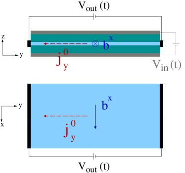
Figure 1: (color online) The Rashba spin-orbit coupling constant $\alpha$ is made time dependent by applying a time dependent gate potential $V_{in}(t)$. The light (blue) area represents a two-dimensional electron gas inside a heterostructure. When an in-plane magnetic field along $x$, $b^{x}$, is also switched on, a charge current $j^{0}_{y}$ flowing along $y$ and proportional to $\dot{\alpha}$ is generated, its actual sign depending on the sign of $\dot{\alpha}$. The induced voltage drop in the transverse direction $V_{out}(t)$ can then be used to measure the strenght of the Rashba interaction.

The Rashba spin-orbit coupling constant $\alpha$ arises from the potential confining the 2DEG and is thus tunable by a gate voltage: if the latter is time dependent, so is the former. Let us then consider the Rashba Hamiltonian for a time-dependent Rashba parameter, $\alpha\rightarrow\alpha(T)$. In the non-Abelian language this means that the $SU(2)$ vector potential becomes time dependent, and therefore a spin dependent electric field is generated. Explicitly we have

$$\gamma\bm{\mathcal{E}} = 2m\dot{\alpha}\left(\sigma^{y}/2,-\sigma^{x}/2,0\right)$$ (74)

$$\gamma\bm{\mathcal{B}} = -\left(2m\alpha\right)^{2}(0,0,\sigma^{z}/2),$$ (75)

with $\dot{\alpha}=\partial_{T}\alpha$. The $SU(2)$ electric field leads to the appearance of in-plane spin currents, as discussed in Ref. [Tang et al., 2005]. However it does not generate a charge current, since it acts with opposite sign on particles with different spin: the net field obtained after averaging over all particles is zero. This is not anymore the case if a magnetic field is also present. Say the latter points in $x$-direction, then a nonzero average electric field in the $y$ direction appears, given by $\gamma\langle{\mathcal{E}}_{y}\rangle=-m\dot{\alpha}\langle\sigma_{x}\rangle=-2m\dot{\alpha}s^{x}/n$ (here $\langle...\rangle$ denotes the average over all particles). We then expect a particle current in $y$-direction of the order $j_{y}=-2DN_{0}\gamma\langle{\mathcal{E}}_{y}\rangle$. We now make the argument quantitative. Let us apply an in-plane Zeeman field along $x$, as shown in Fig. 1. Then the $SU(2)$ electric and magnetic fields are

$$\gamma\bm{\mathcal{E}} = 2m\left(\dot{\alpha}\sigma^{y}/2+\alpha b^{x}\sigma^{z}/2,-\dot{\alpha}\sigma^{x}/2,0\right),$$ (76)

$$\gamma\bm{\mathcal{B}} = -\left(2m\alpha\right)^{2}(0,0,\sigma^{z}/2).$$ (77)

Note that the structure of the Bloch equations (71) is not modified, so that the stationary spin density is

$$s^{x}=s^{x}_{eq},\quad s^{y}=0,\quad s^{z}=0,$$ (78)

with $s^{x}_{eq}=N_{0}b^{x}/2$ as before. As expected, the $SU(2)$ electric field generates a particle current flowing along $y$,

$$j^{0}_{y} = -2D^{x}\frac{N_{0}}{2}\gamma{\mathcal{E}}^{x}_{y}$$ (79)

$$= \tau_{tr}\dot{\alpha}N_{0}b^{x}(1+\gamma_{0}/2),$$

having used $D^{x}=\tau_{tr}/m(1+\gamma_{0}/2)s^{x}$. Finally, for a general direction of the in-plane magnetic field ${\bf b}$ the charge current is given by

$${\bf j}^{0}=\tau_{tr}N_{0}\dot{\alpha}(1+\gamma_{0}/2)\hat{\bf z}\wedge{\bf b}.$$ (80)

Such an effect could provide an alternative way of estimating the strenght of the Rashba interaction, since other spin-orbit mechanisms would not gain any time dependency from a modulated confining potential.

VI Conclusions

We showed how to microscopically derive the generalized Boltzmann and Eilenberger equations in the presence of non-Abelian gauge fields. In the $SU(2)$ case such equations can be used to describe spin-charge coupled dynamics in two-dimensional systems whose Hamiltonians include linear-in-momentum spin-orbit coupling terms. All degrees of freedom are treated symmetrically and the proper identification of the physical quantities follows naturally from the form of the continuity equation. Considering elastic disorder, we obtained results which hold as long as $\epsilon\gg 1/\tau,\Delta_{so}$ and for arbitrary values of $\Delta_{so}\tau$. In particular, we showed that by using the covariant quasiclassical Green function, the collision integral in the kinetic equation is not affected by the gauge fields, which only appear to modify the hydrodynamic derivative. We expect that this nice disentanglement of gauge fields and disorder effects in the Boltzmann and Eilenberger equations may prove very useful when considering quantum correctionsChalaev and Loss (2005, 2009). We also expect the approach to allow for a generalization of the boundary conditions for the Eilenberger equation to the case in which spin and charge channels are coupled. When discussing the diffusive regime, we first obtained Bloch-like equations for the spin and charge, and then exploited them to predict a novel effect. Finally, we note that by making the non-Abelian coupling constant momentum dependent, $\gamma\rightarrow\gamma(\bf p)$, it may be possible to extend the present formalism to include Hamiltonians with more general forms of spin-orbit interaction – i.e. not limited to being linear in momentum.

We thank U. Eckern, J. Rammer and M. Dzierzawa for discussions. This work was supported by the Deutsche Forschungsgemeinschaft through SFB 484 and SPP 1285 and partially supported by EU through PITN-GA-2009-234970.

Appendix A Quasiclassical normalization condition and the collision integral

Consider a quantity $F(1,2)$ which is non-locally covariant, i.e. which under the gauge transformation Eq. (15) transforms according to $F^{\prime}(1,2)=V(1)F(1,2)V^{\dagger}(2)$. Its locally covariant counterpart reads $\tilde{F}(1,2)\equiv U_{\Gamma}(X,1)F(1,2)U_{\Gamma}(2,X)$, where $X=([t_{1}+t_{2}]/2,[{\bf x}_{1}+{\bf x}_{2}]/2)$. In Wigner coordinates, up to $\mathcal{O}(A\partial_{p})$ accuracy, one has

$$\tilde{F}=F-\frac{1}{2}\left\{A\partial_{p},F\right\}.$$ (81)

We define the $\xi$-integrated functions

$$f(\epsilon,\varphi,X) = \frac{i}{\pi}\int\,{\rm d}\xi F({\bf p},\epsilon,X),$$ (82)

$$\tilde{f}(\epsilon,\varphi,X) = \frac{i}{\pi}\int\,{\rm d}\xi\tilde{F}({\bf p},\epsilon,X).$$ (83)

Let us start by assuming for simplicity $A=(0,\bm{\mathcal{A}}^{a}\sigma^{a}/2)$ – that is, we have neither electric nor magnetic fields, only spin-orbit coupling – and setting the $SU(2)$ coupling constant to one, $\gamma=1$. Moreover, the functions $F,\tilde{F}$ are assumed to be peaked at the Fermi surface $\xi=0$ or in its vicinity. Thus, by $\xi$-integrating Eq. (81) by parts one has

$$\tilde{f}=f+\frac{1}{2}\left\{\frac{\bm{\mathcal{A}}\cdot\hat{\bf p}}{p_{F}}-\frac{\bm{\mathcal{A}}\cdot\hat{\bm{\varphi}}}{p_{F}}\partial_{\varphi},f\right\},$$ (84)

with $p_{F}$ the Fermi momentum in the absence of spin-orbit coupling. The presence of a $U(1)$ vector potential can be handled just the same way, whereas the inclusion of the scalar potentials $e\Phi+\Psi^{a}\sigma^{a}/2$ is trivial and amounts to a shift of the energy argument of $f$

$$\tilde{f}=f-\frac{1}{2}\left\{(e\Phi+\Psi)\partial_{\epsilon},f\right\}.$$ (85)

Therefore, in the presence of a general 4-potential $A=(e\Phi+\Psi,e{\bf A}+\bm{\mathcal{A}}^{a}\sigma^{a}/2)$, one has

$$\tilde{f} = f-\frac{1}{2}\left\{(e\Phi+\Psi)\partial_{\epsilon},f\right\}+$$ (86)

$$+\frac{1}{2}\left\{\frac{\left(e{\bf A}+\bm{\mathcal{A}}\right)\cdot\hat{\bf p}}{p_{F}}-\frac{\left(e{\bf A}+\bm{\mathcal{A}}\right)\cdot\hat{\bm{\varphi}}}{p_{F}}\partial_{\varphi},f\right\}.$$

We now use Eqs. (81)-(86) to show

• how the $\xi$-integrated Green’s functions $g$ and $\tilde{g}$ are related, and what this implies for the latter’s normalization;

• that the collision integral Eq. (36) is equivalent to the one appearing in [Shytov et al., 2006].

A.1 About $g$ and $\tilde{g}$

Take $F=\check{G}$. From Eq. (84) one obtains

$$\check{\tilde{g}}=\check{g}+\frac{1}{2}\left\{\frac{\bm{\mathcal{A}}\cdot\hat{\bf p}}{p_{F}}-\frac{\bm{\mathcal{A}}\cdot\hat{\bm{\varphi}}}{p_{F}}\partial_{\varphi},\check{g}\right\},$$ (87)

where we did not write down explicitly all the dependencies, since no confusion should arise. Direct calculations show Raimondi et al. (2006)

$$g^{R,A} = \pm\left(1-\frac{\bm{\mathcal{A}}\cdot\hat{\bf p}}{p_{F}}\right)$$ (88)

$$g^{K}_{eq} = 2\tanh\left(\epsilon/2T\right)\left(1-\frac{\bm{\mathcal{A}}\cdot\hat{\bf p}}{p_{F}}\right),$$ (89)

$T$ being the temperature and the result for the Keldysh component being valid at equilibrium. It follows that to order $|\bm{\mathcal{A}}|/p_{F}$ – i.e. $\Delta_{so}/\epsilon_{F}$ – the locally covariant $\xi$-integrated Green’s function has no $SU(2)$ (spin) structure

$$\tilde{g}^{R,A} = \pm 1$$ (90)

$$\tilde{g}^{K}_{eq} = 2\tanh\left(\epsilon/2T\right)$$ (91)

and satisfies the standard normalization condition $\check{\tilde{g}}^{2}=\check{1}$. Recall this has the meaning of a boundary condition satisfied by $\check{\tilde{g}}$, and so is not affected by the introduction of driving electromagnetic [U(1)] fields Shelankov (1984) or of a Zeeman term. Indeed, we saw that including the scalar potentials $e\Phi$ and $\bm{\Psi}$ simply “shifts” the energy argument of $\tilde{g}^{K}_{eq}$

$$\tilde{g}^{K}_{eq}=\left[1-\frac{1}{2}\left\{(e\Phi+\Psi)\partial_{\epsilon},\;.\;\right\}\right]2\tanh\left(\epsilon/2T\right).$$ (92)

A.2 The collision integral

Take $F=-i[\check{\Sigma},\check{G}]^{K}\equiv C$, and so $\tilde{F}=-i[\check{\tilde{\Sigma}},\check{\tilde{G}}]^{K}\equiv\tilde{C}$. The $\xi$-integration delivers

$$\tilde{c}=-\frac{1}{\tau}\left[\langle K\rangle\tilde{g}^{K}-\langle K\tilde{g}^{K}\rangle\right],$$ (93)

with the kernel $K(\varphi-\varphi^{\prime})\equiv 2\pi N_{0}\tau W(\varphi-\varphi^{\prime})$, and where $\langle...\rangle$ is shorthand for angular average. One then uses the inverse of Eq. (86) to calculate the corresponding expression in the standard (“non-tilde”) language. We consider separately the effects of spin-orbit ($\bm{\mathcal{A}}$) and of a Zeeman field ($\Psi$), since they add linearly.

First, spin-orbit. Starting from

$$c = \tilde{c}-\frac{1}{2}\left\{\frac{\bm{\mathcal{A}}\cdot\hat{\bf p}}{p_{F}}-\frac{\bm{\mathcal{A}}\cdot\hat{\bm{\varphi}}}{p_{F}}\partial_{\varphi},\tilde{c}\right\}$$ (94)

$$= -\frac{1}{\tau}\left[\tilde{g}-\langle K\tilde{g}\rangle\right]+$$

$$-\frac{1}{2\tau}\left\{\frac{\bm{\mathcal{A}}\cdot\hat{\bf p}}{p_{F}}-\frac{\bm{\mathcal{A}}\cdot\hat{\bm{\varphi}}}{p_{F}}\partial_{\varphi},\tilde{g}-\langle K\tilde{g}\rangle\right\},$$

the translation from $\tilde{g}$ to $g$ is done by means of Eq. (84). The calculation is easy but some care is needed, so this is done step by step. First recall that

$$\tilde{g}-\frac{1}{2}\left\{\frac{\bm{\mathcal{A}}\cdot\hat{\bf p}}{p_{F}}-\frac{\bm{\mathcal{A}}\cdot\hat{\bm{\varphi}}}{p_{F}}\partial_{\varphi},\tilde{g}\right\}=g,$$ (95)

so that Eq. (94) becomes

$$c = -\frac{1}{\tau}\left[g-\langle K\tilde{g}\rangle\right]+$$ (96)

$$+\frac{1}{2\tau}\left\{\frac{\bm{\mathcal{A}}\cdot\hat{\bf p}}{p_{F}}-\frac{\bm{\mathcal{A}}\cdot\hat{\bm{\varphi}}}{p_{F}}\partial_{\varphi},\langle Kg\rangle\right\}.$$

Then consider the $\langle K\tilde{g}\rangle$ term, where $K=K(\varphi-\varphi^{\prime})$

$$\langle K\tilde{g}\rangle = \int\,\frac{{\rm d}\varphi^{\prime}}{2\pi}g(\varphi^{\prime})+$$

$$+\frac{1}{2}\int\,\frac{{\rm d}\varphi^{\prime}}{2\pi}\left\{\frac{\bm{\mathcal{A}}\cdot\hat{\bf p}^{\prime}}{p_{F}}K+\frac{\bm{\mathcal{A}}\cdot\hat{\bm{\varphi}}^{\prime}}{p_{F}}K,\partial_{\varphi^{\prime}}g(\varphi^{\prime})\right\}$$

$$= \langle Kg\rangle+$$

$$+\frac{1}{2}\int\,\frac{{\rm d}\varphi^{\prime}}{2\pi}\left\{\left[\frac{\bm{\mathcal{A}}\cdot\hat{\bf p}^{\prime}}{p_{F}}+\frac{\bm{\mathcal{A}}\cdot\left(\partial_{\varphi^{\prime}}\hat{\bm{\varphi}}^{\prime}\right)}{p_{F}}\right]K+\right.$$

$$\left.+\frac{\bm{\mathcal{A}}\cdot\hat{\bm{\varphi}}^{\prime}}{p_{F}}\left[\partial_{\varphi^{\prime}}K\right],g(\varphi^{\prime})\right\}$$

$$= \langle Kg\rangle+\frac{1}{2}\int\,\frac{{\rm d}\varphi^{\prime}}{2\pi}\left\{\frac{\bm{\mathcal{A}}\cdot\hat{\bm{\varphi}}^{\prime}}{p_{F}},\left[\partial_{\varphi^{\prime}}K\right]g(\varphi^{\prime})\right\},$$

having performed a partial integration and used that $g(\varphi=0)=g(\varphi=2\pi),\;\partial_{\varphi^{\prime}}\hat{\bm{\varphi}}^{\prime}=-\hat{\bf p}^{\prime}$. This way Eq.(96) reads

$$c = -\frac{1}{\tau}\left[g-\langle Kg\rangle\right]+\frac{1}{2\tau}\left\{\frac{\bm{\mathcal{A}}\cdot\hat{\bf p}}{p_{F}},\langle Kg\rangle\right\}+$$ (97)

$$-\frac{1}{2\tau}\int\,\frac{{\rm d}\varphi^{\prime}}{2\pi}\left\{\frac{\bm{\mathcal{A}}\cdot\hat{\bm{\varphi}}^{\prime}}{p_{F}},\left[\partial_{\varphi^{\prime}}K\right]g(\varphi^{\prime})\right\}+$$

$$-\frac{1}{2\tau}\left\{\frac{\bm{\mathcal{A}}\cdot\hat{\bm{\varphi}}}{p_{F}}\partial_{\varphi},\langle Kg\rangle\right\}.$$

Now work on the last term. Recall the assumption that the scattering amplitude depend only on the momentum transfer, i.e. $K({\bf p},{\bf p}^{\prime})=K({\bf p}-{\bf p}^{\prime})$. This implies

$$\frac{\hat{\bm{\varphi}}}{p_{F}}\partial_{\varphi}K=-\frac{p_{F}}{m}\hat{\bf p}\partial_{\xi}K-\left[\frac{p_{F}}{m}\hat{\bf p}^{\prime}\partial_{\xi}+\frac{\hat{\bm{\varphi}}^{\prime}}{p_{F}}\partial_{\varphi^{\prime}}\right]K.$$ (98)

From the last term of Eq. (97) one therefore has

$$-\frac{1}{2\tau}\left\{\frac{\bm{\mathcal{A}}\cdot\hat{\bm{\varphi}}}{p_{F}}\partial_{\varphi},\langle Kg\rangle\right\}=\frac{1}{2\tau}\left\{\frac{\bm{\mathcal{A}}\cdot{\bf p}_{0}}{m},\langle\partial_{\xi}Kg\rangle\right\}+$$

$$\frac{1}{2\tau}\langle\left\{\frac{\bm{\mathcal{A}}\cdot{\bf p}_{0}}{m},\partial_{\xi}Kg\right\}\rangle+$$

$$+\frac{1}{2\tau}\int\,\frac{{\rm d}\varphi^{\prime}}{2\pi}\left\{\frac{\bm{\mathcal{A}}\cdot\hat{\bm{\varphi}}^{\prime}}{p_{F}},\left[\partial_{\varphi^{\prime}}K\right]g(\varphi^{\prime})\right\}.$$ (99)

Substitution back into Eq. (97) gives

$$c = -\frac{1}{\tau}\left[g-\langle Kg\rangle\right]+$$ (100)

$$+\frac{1}{2\tau}\left\{\frac{\bm{\mathcal{A}}\cdot\hat{\bf p}}{p_{F}},\langle Kg\rangle\right\}+\frac{1}{2\tau}\left\{\frac{\bm{\mathcal{A}}\cdot{\bf p}_{0}}{m},\langle\partial_{\xi}Kg\rangle\right\}$$

$$+\frac{1}{2\tau}\langle\left\{\frac{\bm{\mathcal{A}}\cdot{\bf p}_{0}}{m},\partial_{\xi}Kg\right\}\rangle.$$

This expression can also be obtained by a direct $\xi$-integration of the collision integral in the standard (“non-tilde”) language. It agrees with the one appearing in [Shytov et al., 2006] for the case of parabolic bands when one identifies ${\bf b}\cdot\bm{\sigma}/2=\bm{\mathcal{A}}\cdot{\bf p}/m$, ${\bf b}$ being the internal spin-orbit field in the language of Ref. [Shytov et al., 2006]. Besides the first two terms, in which no spin-orbit contribution appears, the third term corresponds to corrections due to the spin dependent density of states, whereas the fourth and fifth arise from the energy dependence of the scattering amplitude. In the notation of [Shytov et al., 2006], the former corrections are due to ${\bf M}^{d}$ and the latter to ${\bf M}^{w}$ – notice that some of the ${\bf M}^{d}$ and ${\bf M}^{w}$ contributions cancel each other because of Eq. (98).

Let us now consider a Zeeman field described by the scalar potential $\bm{\Psi}$. Shifting from covariant to non-covariant quantities is done according to Eq. (85) and its inverse. Notice that the kernel $K$ is a function of $\xi$ evaluated at $\xi=\epsilon$. The energy $\epsilon$ is actually sent to zero during the $\xi-$integration, though since we now have to shift back to the non-covariant language it is better to explicitly keep track of this dependency. At the end it will be as usual $\xi=\epsilon\rightarrow 0$. From the inverse of Eq. (85)

$$c(\epsilon)=\tilde{c}(\epsilon)+\frac{1}{2}\left\{\bm{\Psi},\partial_{\epsilon}\tilde{c}(\epsilon)\right\}.$$ (101)

The first term on the r.h.s. gives

$$\tilde{c} = -\frac{1}{\tau}\left[\langle K\rangle g-\langle Kg\rangle\right]+$$ (102)

$$-\frac{1}{2\tau}\left[\langle K\rangle\left\{\bm{\Psi},g^{\prime}\right\}-\langle K\left\{\bm{\Psi},g^{\prime}\right\}\rangle\right],$$

whereas the second one leads to

$$\partial_{\epsilon}\tilde{c}=-\frac{1}{\tau}\left[\langle K^{\prime}\rangle\tilde{g}+\langle K\rangle\tilde{g}^{\prime}-\langle K^{\prime}\tilde{g}\rangle-\langle K\tilde{g}^{\prime}\rangle\right]$$ (103)

where $K^{\prime}=\partial_{\epsilon}K,\tilde{g}^{\prime}=\partial_{\epsilon}\tilde{g}$. Plugging both expressions into Eq. (101) one has

$$c(\epsilon) = -\frac{1}{\tau}\left[\langle K\rangle g-\langle Kg\rangle\right]+$$ (104)

$$+\frac{1}{2\tau}\left[\langle K\rangle\left\{\bm{\Psi},g^{\prime}\right\}-\langle K\left\{\bm{\Psi},g^{\prime}\right\}\rangle\right]+$$

$$-\frac{1}{2\tau}\left[\langle K^{\prime}\rangle\left\{\bm{\Psi},g\right\}+\langle K\rangle\left\{\bm{\Psi},g^{\prime}\right\}+\right.$$

$$\quad\quad\left.-\langle K^{\prime}\left\{\bm{\Psi},g\right\}\rangle-\langle K\left\{\bm{\Psi},g^{\prime}\right\}\rangle\right]$$

$$= -\frac{1}{\tau}\left[\langle K\rangle g-\langle Kg\rangle\right]+$$

$$-\frac{1}{2\tau}\left\{\bm{\Psi},\langle K^{\prime}\rangle g-\langle K^{\prime}g\rangle\right\}$$

with $g=g(\epsilon),g^{\prime}=\partial_{\epsilon}g$ and $K,K^{\prime}$ are evaluated at the Fermi surface $\xi=\epsilon=0$. The full expression for the scattering kernel in the presence of spin-orbit coupling and a Zeeman field is given by the sum of Eq. (100) and Eq. (104). It leads to results in agreement with Ref. [Engel et al., 2007].

References

- Žutić et al. (2004) I. Žutić, J. Fabian, and S. D. Sarma, Rev. Mod. Phys., 76, 323 (2004).
- Awschalom and Flatté (2007) D. D. Awschalom and M. Flatté, Nat. Phys., 3, 153 (2007).
- Inoue et al. (2009) J.-I. Inoue, T. Kato, G. E. W. Bauer, and L. W. Molenkamp, Semicond. Sci. Technol., 24, 064003 (2009).
- Engel et al. (2007) H. Engel, E. Rashba, and B. Halperin, in Handbook of Magnetism and Advanced Magnetic Materials, edited by H. Kronmüller and S. Parkin (John Wiley Sons Ltd, Chichester, UK, 2007) p. 2858.
- Sinitsyn (2008) N. A. Sinitsyn, J. Phys.: Condens. Matter, 20, 023201 (2008).
- Nagaosa et al. (2010) N. Nagaosa, J. Sinova, S. Onoda, A. H. MacDonald, and N. P. Ong, Rev. Mod. Phys., 82, 1539 (2010).
- Ziman (1972) J. M. Ziman, Principles of the Theory of Solids, 2nd ed. (Cambridge University Press, 1972).
- Khaetskii (2006) A. Khaetskii, Phys. Rev. Lett., 96, 056602 (2006).
- Trushin and Schliemann (2007) M. Trushin and J. Schliemann, Phys. Rev. B, 75, 155323 (2007).
- Kailasvuori (2009) J. Kailasvuori, J. Stat. Mech., P08004 (2009).
- Mishchenko et al. (2004) E. G. Mishchenko, A. V. Shytov, and B. I. Halperin, Phys. Rev. Lett., 93, 226602 (2004).
- Shytov et al. (2006) A. V. Shytov, E. G. Mishchenko, H.-A. Engel, and B. I. Halperin, Phys. Rev. B, 73, 075316 (2006).
- Raimondi et al. (2006) R. Raimondi, C. Gorini, P. Schwab, and M. Dzierzawa, Phys. Rev. B, 74, 035340 (2006).
- Sundaram and Nyu (1999) G. Sundaram and Q. Nyu, Phys. Rev. B, 59, 14915 (1999).
- Sinitsyn et al. (2007) N. A. Sinitsyn, A. H. MacDonald, T. Jungwirth, V. K. Dugaev, and J. Sinova, Phys. Rev. B, 75, 045315 (2007).
- Mathur and Stone (1992) H. Mathur and A. D. Stone, Phys. Rev. Lett., 68, 2964 (1992).
- Fröhlich and Studer (1993) J. Fröhlich and U. M. Studer, Rev. Mod. Phys., 65, 733 (1993).
- Jin et al. (2006) P.-Q. Jin, Y.-Q. Li, and F.-C. Zhang, J. Phys. A, 39, 7115 (2006).
- Bernevig et al. (2006) B. A. Bernevig, J. Orenstein, and S.-C. Zhang, Phys. Rev. Lett., 97, 236601 (2006).
- Hatano et al. (2007) N. Hatano, R. Shirasaki, and H. Nakamura, Phys. Rev. A, 75, 032107 (2007).
- Tokatly (2008) I. V. Tokatly, Phys. Rev. Lett., 101, 106601 (2008).
- Tokatly and Sherman (2010) I. V. Tokatly and E. Y. Sherman, Ann. Phys., 325, 1104 (2010).
- Duckheim et al. (2009) M. Duckheim, D. L. Maslov, and D. Loss, Phys. Rev. B, 80, 235327 (2009).
- Koralek et al. (2009) J. D. Koralek, C. P. Weber, J. Orenstein, B. A. Bernevig, S.-C. Zhang, S. Mack, and D. D. Awschalom, Nature, 458, 610 (2009).
- Wunderlich et al. (2009) J. Wunderlich, A. C. Irvine, J. Sinova, B. G. Park, L. P. Zârbo, X. L. Xu, B. Kaestner, V. Novák, and T. Jungwirth, Nature Physics, 5, 675 (2009).
- Osterloh et al. (2005) K. Osterloh, M. Baig, L. Santos, P. Zoller, and M. Lewenstein, Phys. Rev. Lett., 95, 010403 (2005).
- Günther et al. (2009) K. J. Günther, M. Cheneau, T. Yefsah, S. P. Rath, and J. Dalibard, Phys. Rev. A, 79, 011604(R) (2009).
- Liu et al. (2009) X.-J. Liu, M. F. Borunda, X. Liu, and J. Sinova, Phys. Rev. Lett., 102, 046402 (2009).
- Merkl et al. (2010) M. Merkl, G. Juzeliunas, and P. Öhberg, arXiv:0912.3417 (2010).
- Lee et al. (2009) M. Lee, M. O. Hachiya, E. Bernardes, J. C. Egues, and D. Loss, Phys. Rev. B, 80, 155314 (2009).
- Note (1) In this case the Hamiltonian can be written introducing – rather than – gauge fields.
- Keldysh (1964) L. V. Keldysh, Zh. Eksp. Teor. Fiz., 47, 1515 (1964), [Sov. Phys. – JETP v.20, p. 1018 (1965)].
- Shindou and Balents (2008) R. Shindou and L. Balents, Phys. Rev. B, 77, 035110 (2008).
- Rammer and Smith (1986) J. Rammer and H. Smith, Rev. Mod. Phys., 58, 323 (1986).
- Prange and Kadanoff (1964) R. E. Prange and L. P. Kadanoff, Phys. Rev., 134, A 566 (1964).
- Schwab and Raimondi (2003) P. Schwab and R. Raimondi, Ann. Phys., 471, 12 (2003).
- Langreth (1966) D. C. Langreth, Phys. Rev., 148, 707 (1966).
- Altshuler (1978) B. L. Altshuler, JETP, 48, 670 (1978).
- Peskin and Schroeder (1995) M. E. Peskin and D. V. Schroeder, An Introduction to Quantum Field Theory (Perseus Books, 1995).
- Note (2) Since the gauge transformation properties do not depend on the choice of , we pick the simplest curve.
- Note (3) This corresponds to a “next-to-leading-order” expansion and is necessary to couple Abelian and non-Abelian fields to one another. In the physically more transparent language of spin-orbit coupling, the terms order are those that produce spin-charge coupling – and thus lead to, say, the spin Hall effect or the anomalous Hall effect.
- Dyakonov and Perel (1971) M. I. Dyakonov and V. I. Perel, Phys. Lett., 35A, 459 (1971).
- Hirsch (1999) J. E. Hirsch, Phys. Rev. Lett., 83, 1834 (1999).
- Nozières and Lewiner (1973) P. Nozières and C. Lewiner, J. Phys., France, 34, 901 (1973).
- Engel et al. (2005) H.-A. Engel, B. I. Halperin, and E. I. Rashba, Phys. Rev. Lett., 95, 166605 (2005).
- Hankiewicz and Vignale (2008) E. M. Hankiewicz and G. Vignale, Phys. Rev. Lett., 100, 026602 (2008).
- Raimondi and Schwab (2009) R. Raimondi and P. Schwab, EPL, 87, 37008 (2009).
- Eckern and Schmid (1981) M. Eckern and A. Schmid, JLTP, 45, 137 (1981).
- Shelankov (1984) A. L. Shelankov, J.Low Temp. Phys., 60, 29 (1984).
- Zaitsev (1984) A. V. Zaitsev, Sov. Phys. JETP, 59, 1015 (1984).
- Millis et al. (1988) A. Millis, D. Rainer, and J. A. Sauls, Phys. Rev. B, 38, 4504 (1988).
- Eschrig (2009) M. Eschrig, Phys. Rev. B, 80, 134511 (2009).
- Engel et al. (2007) H.-A. Engel, E. I. Rashba, and B. I. Halperin, Phys. Rev. Lett., 98, 036602 (2007b).
- Milletarì et al. (2008) M. Milletarì, R. Raimondi, and P. Schwab, EPL, 82, 67005 (2008).
- Note (4) Notice that the above does not agree with the results found in Ref. [\rev@citealpnummilletari2008], though the discrepancy is no surprise: in [\rev@citealpnummilletari2008] a different model of disorder was used, one in which the dependence of the scattering amplitude on the modulus of the momentum was neglected.
- Tang et al. (2005) C. S. Tang, G. A. Mal’shukov, and K. A. Chao, Phys. Rev. B, 71, 195314 (2005).
- Chalaev and Loss (2005) O. Chalaev and D. Loss, Phys. Rev. B, 71, 245318 (2005).
- Chalaev and Loss (2009) O. Chalaev and D. Loss, Phys. Rev. B, 80, 035305 (2009).