Measurement back-action on adiabatic coherent electron transport

Abstract

We study the back-action of a nearby measurement device on electrons undergoing coherent transfer via adiabatic passage (CTAP) in a triple-well system. The measurement is provided by a quantum point contact capacitively coupled to the middle well, thus acting as a detector sensitive to the charge configuration of the triple-well system. We account for this continuous measurement by treating the whole $\{$triple-well + detector$\}$ as a closed quantum system. This leads to a set of coupled differential equations for the density matrix of the enlarged system which we solve numerically. This approach allows to study a single realization of the measurement process while keeping track of the detector output, which is especially relevant for experiments. In particular, we find the emergence of a new peak in the distribution of electrons that passed through the point contact. As one increases the coupling between the middle potential well and the detector, this feature becomes more prominent and is accompanied by a substantial drop in the fidelity of the CTAP scheme.

Solid-state based quantum computer architectures are currently the focus of active experimental and fundamental research, as many of them offer the promise of being scalable, therefore opening the way to significant improvements in efficiency of certain algorithms. An essential feature of many proposals for scalable quantum computation is the coherent transport over large distances of quantum information, encoded e.g. in electron spins.

A recent method of all-electrical population transfer for electrons has been suggested in solid-state systems consisting of a chain of potential wells greentree . Termed Coherent Transfer by Adiabatic Passage or CTAP, this technique is a spatial analogue of the STImulated Raman Adiabatic Passage (STIRAP) protocol stirap used in quantum optics to transfer population between two long-lived atomic or molecular energy levels. The CTAP scheme amounts to transporting electrons coherently from one end of the chain to the other by dynamically manipulating the tunnel barriers between the successive potential wells. For the appropriate driving of the system, this method ensures that the occupation in the middle of the chain is exponentially suppressed at any point of time.

There have been several proposals to perform the CTAP scheme in triple-well solid-state systems such as quantum dots schoerer ; qdot-proposal ; Cole2008 ; Das2009 , ionized donors PinSi-proposal or superconductors sc-proposal . Similarly, this technique has been put forward as a means to transport single atoms coldatoms-proposal and Bose-Einstein condensates bec-proposal within optical potentials. Recently, a classic analogue of CTAP has also been demonstrated experimentally, using photons in a triple-well optical waveguide photons . The CTAP protocol therefore has both a quantum optics and a condensed matter version, thus raising interest well beyond the field of quantum information.

The implementation of the CTAP protocol naturally brings about the question of its observation. The most striking signature of CTAP is the vanishing occupation of the middle potential well, which can be monitored using a sensitive electrometer. In solid-state devices, this is usually achieved using ballistic quantum point contacts (QPC). The electric current flowing through the QPC is influenced by the presence of an electronic charge in its close environment, thus turning the QPC into a charge detector. While this could provide a good test for the observation of CTAP, one may wonder to what extent this charge detection is invasive. This is also directly relevant for possible applications of the CTAP scheme for quantum information purposes: measurement back-action in the above setup can be related to the influence of a decohering environment along the chain.

Now it is largely believed that the CTAP scheme is relatively robust against this type of measurements precisely because the middle potential well is barely populated. However, recent work decoherence concentrating on the decoherence aspects associated with nonlocal measurements suggests otherwise. In this Letter, we study the measurement back-action of the QPC on the CTAP scheme, focusing on the effects of a continuous measurement process. While the measurement process is instantaneous for optical experiments, it can take a significant amount of time for typical solid-state setups and therefore leads to such a continuous evolution of the system subjected to it. The continuous measurement thus poses a non-trivial time-dependent problem, complicated by the dynamic tuning of the tunneling rates between potential wells. Our approach closely follows an alternative derivation of the Bayesian formalism developed by Korotkov korotkov . The advantages over the conventional master equation are two-fold. First, it allows for the analysis of a particular realization of the measurement process, rather than capturing the behavior of the system averaged over many measurements. Second, it enables us to keep track of the detector output over the duration of the transfer, providing us with information about the time evolution of the system, relevant to upcoming experiments.

We consider a triple-well solid-state system, whose Hamiltonian is characterized by the time-dependent tunneling rate $\Omega_{ij}(t)$ between wells $i$ and $j$, and the energy $\epsilon$ of the potential wells:

$$H_{3w}=\sum_{i=1}^{3}\epsilon c_{i}^{\dagger}c_{i}+\left(\hbar\Omega_{12}(t)c_{1}^{\dagger}c_{2}+\hbar\Omega_{23}(t)c_{2}^{\dagger}c_{3}+\rm{h.c.}\right),$$ (1)

where $c_{i}^{\dagger}$ creates an electron in well $i$.

We now wish to apply the CTAP scheme to coherently transfer an electron from well 1 to well 3. Following Ref. greentree, , this is achieved by applying Gaussian voltage pulses to tune the tunnel barriers in time according to

$$\Omega_{12}(t) = \Omega_{\rm max}\exp\left[-\frac{(t-t_{\rm max}/2-t_{\rm delay})^{2}}{2\sigma^{2}}\right]$$

$$\Omega_{23}(t) = \Omega_{\rm max}\exp\left[-\frac{(t-t_{\rm max}/2)^{2}}{2\sigma^{2}}\right],$$ (2)

where we introduced the pulses height ($\Omega_{\rm max}$) and duration ($t_{\rm max}$), and chose for the standard deviation $\sigma=t_{\rm max}/8$. The delay between pulses is selected in order to optimize the transfer, $t_{\rm delay}=2\sigma$ delay . Like in the STIRAP protocol, the pulses are applied in a counter-intuitive sequence, where $\Omega_{23}$ is fired prior to $\Omega_{12}$, in order to maximize the fidelity of the transfer greentree .

To monitor the charge configuration of this system, we couple the middle potential well to a charge detector. Here we use a simplified version of the QPC, namely a tunnel junction whose barrier height is sensitive to the presence of an electron in the middle well. The hopping amplitude through the barrier varies from $\Omega^{\prime}$ to $\Omega$, depending on whether or not well 2 is occupied gurvitz . The detector Hamiltonian can thus be written as

$$H_{qpc} = \sum_{r}E_{r}:a_{r}^{\dagger}a_{r}:+\sum_{l}E_{l}:a_{l}^{\dagger}a_{l}:$$ (3)

$$+\sum_{l,r}\hbar\left(\Omega+\delta\Omega~{}c_{2}^{\dagger}c_{2}\right)(a_{r}^{\dagger}a_{l}+a_{l}^{\dagger}a_{r}),$$

where $a_{r}^{\dagger}$ and $a_{l}^{\dagger}$ are the electron creation operators in the right and left electrode respectively, while $E_{r,l}$ stands for the set of energy levels in the reservoirs. Here we introduced $\delta\Omega=\Omega^{\prime}-\Omega$, and assumed all tunneling amplitudes to be real and independent of the states in the electrodes.

Our goal is to study the evolution of the triple-well system under continuous measurement by the detector, focusing on a single realization of the measurement process. This is achieved by considering the triple-well system and the detector as the two parts of an enlarged quantum system. This allows for describing the quantum state of this enlarged system via a generalized density matrix $\rho_{ij}^{n}$(t) gurvitz . The latter corresponds to the density matrix in the basis of localized states (associated with wells 1, 2, and 3) further divided into components with different number $n$ of electrons passed through the detector. The evolution of this generalized density matrix is given by a set of Bloch-type equations obtained from the many-body Schrödinger equation for the entire system. Extending the derivation of Ref. gurvitz, to include time-dependent tunneling rates, one obtains the following set of rate equations for the density matrix

$$\dot{\rho}_{11}^{n}(t) = D\left[\rho_{11}^{n-1}(t)-\rho_{11}^{n}(t)\right]-2\Omega_{12}(t){\rm Im}\left[\rho_{12}^{n}(t)\right]$$

$$\dot{\rho}_{22}^{n}(t) = D^{\prime}\left[\rho_{22}^{n-1}(t)-\rho_{22}^{n}(t)\right]+2\Omega_{12}(t){\rm Im}\left[\rho_{12}^{n}(t)\right]$$

$$-2\Omega_{23}(t){\rm Im}\left[\rho_{23}^{n}(t)\right]$$

$$\dot{\rho}_{33}^{n}(t) = D\left[\rho_{33}^{n-1}(t)-\rho_{33}^{n}(t)\right]+2\Omega_{23}(t){\rm Im}\left[\rho_{23}^{n}(t)\right]$$

$$\dot{\rho}_{12}^{n}(t) = \sqrt{DD^{\prime}}\rho_{12}^{n-1}(t)-\frac{D+D^{\prime}}{2}\rho_{12}^{n}(t)$$

$$+i\Omega_{12}(t)\left[\rho_{11}^{n}(t)-\rho_{22}^{n}(t)\right]+i\Omega_{23}(t)\rho_{13}^{n}(t)$$

$$\dot{\rho}_{23}^{n}(t) = \sqrt{DD^{\prime}}\rho_{23}^{n-1}(t)-\frac{D+D^{\prime}}{2}\rho_{23}^{n}(t)$$

$$+i\Omega_{23}(t)\left[\rho_{22}^{n}(t)-\rho_{33}^{n}(t)\right]-i\Omega_{12}(t)\rho_{13}^{n}(t)$$

$$\dot{\rho}_{13}^{n}(t) = D\left[\rho_{13}^{n-1}(t)-\rho_{13}^{n}(t)\right]+i\Omega_{23}(t)\rho_{12}^{n}(t)$$ (4)

$$-i\Omega_{12}(t)\rho_{23}^{n}(t),$$

where we used the convention $\rho_{ij}^{0}(t)=0$, and introduced the tunneling rates $D=2\pi\hbar\rho_{R}\rho_{L}\Omega^{2}eV$ and $D^{\prime}=2\pi\hbar\rho_{R}\rho_{L}\Omega^{\prime 2}eV$. Here we considered a QPC under a voltage bias $V$, with constant density of states $\rho_{R,L}$ in the electrodes. Note that by tracing over the detector degrees of freedom, one recovers the conventional master equation for the density matrix $\rho_{ij}=\sum_{n}\rho_{ij}^{n}$. In this case, the measurement back-action reduces to a constant dephasing term $\Gamma=(\sqrt{D}-\sqrt{D^{\prime}})^{2}/2$, which only affects the coherences $\rho_{12}$ and $\rho_{23}$.

The drawback in including the detector into the quantum part of the setup is that one now needs a way to extract classical information from it. Following Ref. korotkov, , we introduce a classical pointer which periodically collapses the wavefunction of the quantum system. The pointer only interacts with the detector at times $t_{k}$, forcing it to choose a definite value $n_{k}$ for the number $n(t_{k})$ of electrons that passed through the QPC. The value of $n_{k}$ is picked randomly according to the probability distribution $P(n)$ set by the density matrix at the time of the collapse, namely $P(n)=\rho_{11}^{n}(t_{k})+\rho_{22}^{n}(t_{k})+\rho_{33}^{n}(t_{k})$. Once a particular $n_{k}$ has been selected, the density matrix should be immediately updated

$$\rho_{ij}^{n}(t_{k}^{+})=\delta_{n,n_{k}}\frac{\rho_{ij}^{n_{k}}(t_{k}^{-})}{\rho_{11}^{n_{k}}(t_{k}^{-})+\rho_{22}^{n_{k}}(t_{k}^{-})+\rho_{33}^{n_{k}}(t_{k}^{-})}.$$ (5)

After that, the system evolves according to Eq. (4) until the next collapse at $t=t_{k+1}$. While it is not clear how frequently the collapse procedure should occur, we could check explicitly that our results are insensitive to the choice of $t_{k}$, provided that $\Delta t_{k}=t_{k}-t_{k-1}\ll t_{\rm max}$.

The combination of the coupled Bloch equations (4) with the collapse procedure (5) makes the problem difficult to solve analytically. Instead, we propose a solution by stochastic sampling, a method designed to mimic the experimental setup. For a given sequence of times $t_{k}$, we numerically implement the succession of evolutions and collapses while keeping track of the detector output, i.e. the number of electrons $n(t)$ that passed through the QPC. This provides us with one particular realization of the measurement process. In particular, this implies that by the end of the “simulated experiment” at $t=\tau$, one obtains a definite answer whether the electron sits in the middle well or not, so that $\rho_{22}^{n(\tau)}(\tau)$ can only take the values 0 or 1. Moreover, reproducing this procedure over thousands of realizations allows us to extract statistical properties, such as the distribution ${\cal P}(n)$ of the total number of electrons that crossed the tunnel junction over the duration $\tau$ of the experiment. Such features could be qualitatively compared to experimental data when the latter becomes available.

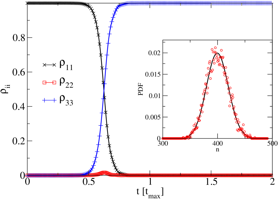
Figure 1: Comparison between $\rho_{ii}(t)$ (lines) and $\rho_{ii}^{n_{k}}(t_{k})$ (symbols), for $\Omega_{\rm max}=80$ and $D=D^{\prime}=200$ (in units of $t_{\rm max}^{-1}$) and $\tau=2t_{\rm max}$. Inset: Distribution ${\cal P}(n)$ of the total number of electrons that crossed the detector over the duration of the experiment, obtained for 5000 runs (symbols). The black curve corresponds to the expected Poisson distribution

As a first test of the method, we consider the case of a decoupled detector, obtained by setting equal tunneling rates $D=D^{\prime}$ in Eq. (4). In this case, no information on the position of the electron can be extracted from the measurement and the CTAP scheme works with optimum fidelity. Turning to the detector output, we plot as an inset in Fig. 1 the distribution ${\cal P}(n)$ obtained after a few thousand runs, which turns out to be very close to the expected Poisson behavior. Furthermore, the profile of the diagonal density matrix $\rho_{ii}^{n_{k}}(t_{k}^{+})$ is identical to the one obtained from solving the conventional master equation for $\rho_{ii}(t)$ with Hamiltonian $H_{3w}$ (1), see Fig. 1.

(a)

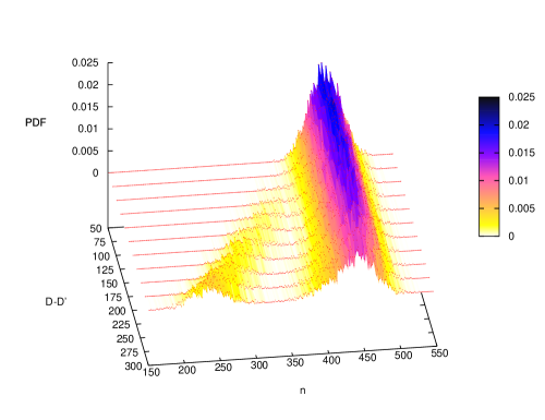
(b)

Figure 2: Distribution ${\cal P}(n)$ as a function of (a) $D-D^{\prime}$ with $\Omega_{\rm max}=50$, $D=300$ (in units of $t_{\rm max}^{-1}$), (b) $\Omega_{\rm max}$, for $D=300$, $D^{\prime}=100$ (in units of $t_{\rm max}^{-1}$). In both cases, the duration of the experiment is $\tau=1.5t_{\rm max}$.

Let us now increase the coupling to the detector, by reducing the value of the tunneling rate $D^{\prime}$ compared to $D$. Keeping track of the distribution ${\cal P}(n)$ of the number of electrons in the detector as a function of the rate mismatch $D-D^{\prime}$ leads to the results of Fig. 2a. The main signature of the measurement back-action on this distribution is the emergence of a satellite peak on top of the Poisson-like behavior. As one increases the value of $D-D^{\prime}$, making the measurement stronger, this secondary structure becomes more prominent, while the main peak flattens out. The distance between these two features grows like $(D-D^{\prime})\tau$. Note that while the peaks are well-separated for longer times $\tau$, they are also more spread out. Out of the thousands of realizations that result in the distribution of Fig. 2a, the ones that contribute to the satellite peak correspond to situations for which the electron sits in the middle well by the end of the experiment, i.e. $\rho_{22}^{n(\tau)}(\tau)=1$. As a result, the integral under this secondary peak measures the proportion $p_{2}$ of runs where the electron is detected in well 2. Obviously, these realizations exemplify an unsuccessful transfer, and one would thus expect a reduced fidelity for the CTAP scheme. Indeed, as the coupling to the detector becomes more important, one obtains more information on the location of the electron, and the fidelity of the CTAP protocol decreases, as shown in Fig. 3a. This reduction turns out to be more important than one would anticipate because the average probability $p_{1}$ of finding the electron in the first potential well is not only finite but also increases along with $D-D^{\prime}$ in a way that $p_{1}\simeq p_{2}$, see Fig. 3a. The measurement therefore leads to an increased population of the middle well, compared to the unmonitored CTAP scheme. This effect is qualitatively similar to that of pure dephasing greentree .

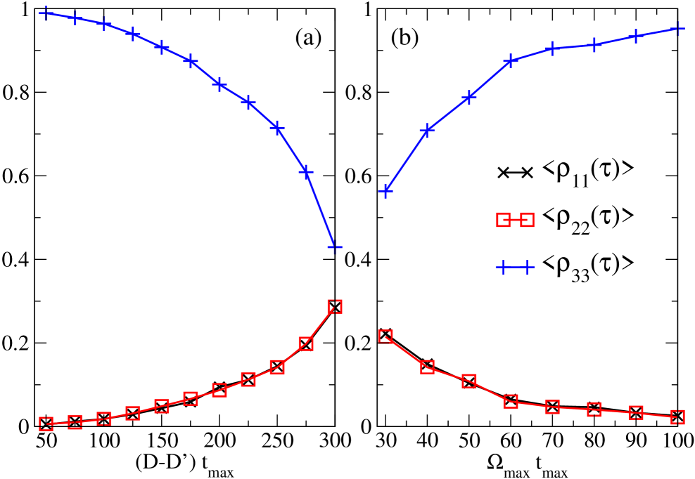
Figure 3: Diagonal part of the density matrix $\rho_{ii}^{n(\tau)}(\tau)$ averaged over all runs, as a function of (a) $D-D^{\prime}$ with $\Omega_{\rm max}=50$, $D=300$ (in units of $t_{\rm max}^{-1}$), (b) $\Omega_{\rm max}$, for $D=300$, $D^{\prime}=100$ (in units of $t_{\rm max}^{-1}$). In both cases, the duration of the experiment is $\tau=1.5t_{\rm max}$.

We could further check that for a given value of $D-D^{\prime}$ increasing the amplitude $\Omega_{\rm max}$ of the pulses restores the fidelity of the CTAP protocol, as illustrated in Fig. 3b. This however goes with a significant loss of weight of the satellite peak in the probability distribution ${\cal P}(n)$ (see Fig. 2b) corresponding to a loss of information on the location of the electron. These results also confirm that the position of the satellite peak is independent of $\Omega_{\rm max}$.

The compiled record of the detector output $n(t)$ for 1000 runs is plotted in Fig. 4, and one readily sees that it can be divided into two subsets. The lower subset is associated with the ensemble of runs that contribute to the satellite peak in ${\cal P}(n)$, and correspond to the detection of the electron in the middle well, $\rho_{22}^{n(\tau)}(\tau)=1$. The upper subset is associated with the ensemble of runs contributing to the main Poisson-like structure in ${\cal P}(n)$, and correspond to $\rho_{22}^{n(\tau)}(\tau)=0$. It is instructive to evaluate the average behavior of $n(t)$ within each of these subsets (see inset of Fig. 4). On average, for the upper subset one has $\langle n(t)\rangle\sim Dt$ over the whole duration of the experiment. For the lower subset, however, there are three distinct regimes, defined by the typical scales $t_{\rm max}$ and $t_{\rm cross}$ (defined as $\Omega_{12}(t_{\rm cross})=\Omega_{23}(t_{\rm cross})$). For $0\leq t\lesssim t_{\rm cross}$, the average number $\langle n(t)\rangle$ of electrons through the detector is again given by $Dt$ and the average occupation of the middle well stays much lower than 1. For times $t\gtrsim t_{\rm max}$, $\langle n(t)\rangle$ grows like $D^{\prime}t$ and the average occupation of the middle well stays close to 1, over the whole time range: the electron has been detected. The most interesting behavior occurs for $t_{\rm cross}\lesssim t\lesssim t_{\rm max}$: the detection builds up as the average occupation of the middle well rises from nearly 0 to nearly 1. In the meantime, the average detector output $\langle n(t)\rangle$ grows like $(D+D^{\prime})t/2$, while one might have expected a gradual decrease of the slope from $D$ to $D^{\prime}$.

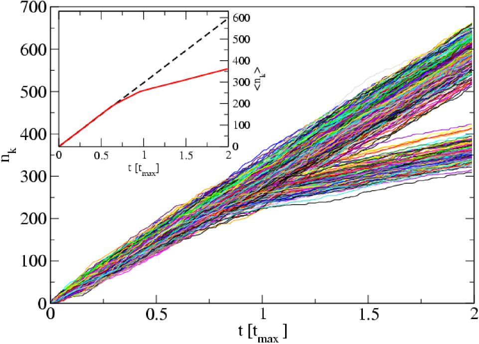
Figure 4: Compiled (main graph) and averaged (inset) record for the upper and lower subsets, obtained for 1000 runs, with with $\Omega_{\rm max}=50$, $D=300$, $D^{\prime}=100$ (in units of $t_{\rm max}^{-1}$) and a duration of the experiment is $\tau=2t_{\rm max}$.

Our results can easily be extended to other pulse shapes and sequences as well as more complicated setups. Our approach also offers the possibility to reconstruct the density matrix from a given experimental measurement record of $n(t)$, by replacing the random collapse procedure with the provided record from the experiment

In summary, we have proposed an approach which allows to study the measurement back-action on an electron submitted to the CTAP protocol in a triple-well system. Our work captures the loss of fidelity of the CTAP scheme associated with the measurement process, a feature generally accounted for in the conventional master equation formalism by explicitly adding a dephasing term. The key observation of this Letter is that the reduction of the fidelity is directly connected to the amount of information one can extract concerning the location of the electron. This has the important implication that a decohering environment coupling to an electron on the CTAP chain reduces the fidelity of this scheme for quantum information transfer in spite of the fact that the occupation probability along the chain can be made arbitrarily small for the case without decoherence.

We are grateful to J.H. Cole, A. Korotkov and S. Ludwig for helpful discussions. This work was supported through SFB 631 of the Deutsche Forschungsgemeinschaft, the Center for NanoScience (CeNS) Munich, and the German Excellence Initiative via the Nanosystems Initiative Munich (NIM).

References

- (1) A.D. Greentree et al., Phys. Rev. B 70, 235317 (2004).
- (2) N.V. Vitanov et al., Annu. Rev. Phys. Chem. 52, 763 (2001).
- (3) D. Schörer et al. , Phys. Rev. B 76, 075306 (2007).
- (4) D. Petrosyan and P. Lambropoulos, Opt. Comm. 264, 419 (2006).
- (5) J.H. Cole et al., Phys. Rev. B 77, 235418 (2008).
- (6) T. Opatrny and K.K. Das, Phys. Rev. A 79, 012113 (2009).
- (7) R. Rahman et al., Phys. Rev. B 80, 035302 (2009).
- (8) J. Siewert, T. Brandes and G. Falci, Opt. Comm. 264, 435 (2006).
- (9) K. Eckert et al., Phys. Rev. A 70, 023606 (2004); K. Eckert et al., Opt. Comm. 264, 264 (2006)
- (10) E.M. Graefe, H.J. Korsch and D. Witthaut, Phys. Rev. A 73, 013617 (2006); M. Rab et al., Phys. Rev. A 77, 061602(R) (2008).
- (11) S. Longhi et al., Phys. Rev. B 76, 201101 (2007).
- (12) I. Kamleitner, J. Cresser and J. Twamley, Phys. Rev. A 77, 032331 (2008).
- (13) A.N. Korotkov, Phys. Rev. B 63, 115403 (2001); A.N. Korotkov, in Quantum Noise in Mesoscopic Physics, edited by Yu.V. Nazarov (Kluwer, Netherlands, 2003), p. 205
- (14) U. Gaubatz et al., J. Chem. Phys. 92, 5363 (1990).
- (15) S.A. Gurvitz, Phys. Rev. B 56, 15215 (1997).
- (16) L.C.L. Hollenberg et al., Phys. Rev. B 74, 045311 (2006); A.D. Greentree, S.J. Devitt and L.C.L. Hollenberg, Phys. Rev. A 73, 032319 (2006).
- (17) S.A. Gurvitz and Ya.S. Prager, Phys. Rev. B 53, 15932 (1996).