Relaxation dynamics of the electron distribution in the Coulomb blockade problem

Abstract

We study the relaxation dynamics of electron distribution function on the island of a single electron transistor. We focus on the regime of not very low temperatures in which an electron coherence can be neglected but quantum fluctuations of charge are strong due to Coulomb interaction. The quantum kinetic equation governing evolution of the electron distribution function due to escape of electrons to the reservoirs is derived. Analytical solutions for time-dependence of the electron distribution are obtained in the regimes of weak and strong Coulomb blockade. We find that usual exponential in time relaxation is strongly modified due to the presence of Coulomb interaction.

I Introduction

Recently, the phenomenon of Coulomb blockade in single electron devices zaikin ; ZPhys ; grabert ; aleiner ; Glazman has come into the focus of the field of thermoelectricity. Giazotto_review Among significant experimental achievements one can list development of the Coulomb blockade thermometer, Giazotto_review the thermal rectifier on the basis of a quantum dot, ScheibnerNew new technique to measure temperature gradients across a quantum dot, Hoffmann etc. The standard characteristic of thermoelectric performance is the figure of merit which involves the product of conductance, thermopower squared and inverse thermal conductance. Measurements of thermopower and thermal conductance in single electron transistors (SET) and quantum dots have been performed during the last decade at different temperature regimes. Dzurak ; Scheibner ; Moeller The theory of the thermoelectric effects in electron devices has been put forward in Refs. [Amman, ; BeenakkerStaring, ]. During the last decade the thermopower and thermal conductance have been studied in single electron transistors and quantum dots, AndreevMatveev ; TurekMatveev ; MatveevAndreev1 ; kubala1 ; Nakanishi ; Zianni ; kubala2 and in granular metals beloborodov0 ; TripathiLoh ; beloborodov1 ; beloborodov2 ; beloborodov3 in various regimes. However, the thermopower and thermal conductance are linear response parameters and, therefore, describe the equilibrium properties of a system only.

In contrast, our work is focused on properties of single electron devices in the out-of-equilibrium regime which has attracted a lot of theoretical interest recently. In particular, the conductance of a quantum dot under ac pumping in the stationary non-equilibrium state was obtained in Ref. [BaskoKravtsov, ], the current noise of an ac-biased quantum dot was studied in Ref. [Bagrets, ], the non-equilibrium dephasing rate and zero-bias anomaly in single electron transistor was computed in Ref. [AltlandEgger, ], the statistics of temperature and current fluctuations in the fully out-of equilibrium single electron transistor was investigated in Refs. [nazarov1, ; nazarov2, ], and the extension of the $P(E)$-theory NazPE to the out-of-equilibrium regime has been developed in Refs. [K1, ; K2, ]. However, these works dealt with regimes when the distribution function of electrons in a quantum dot or an island of single electron transistor were fixed by external sources, e.g., ac or dc bias voltage.

In this paper we address a different question: how does an electron distribution function once being prepared relaxes toward the equilibrium state in the Coulomb blockade problem. Apart from general physical interest in understanding of a non-equilibrium regime, the answer to this question is important for the field of electron thermometry. Giazotto_review

We consider the simplest system: single electron transistor. The set-up is shown schematically in Fig. 1. Metallic island is coupled to an equilibrium electron reservoirs via tunneling junctions. Depending on the task, the reservoirs and the island may be kept at different temperatures ($T_{l}$, $T_{r}$ respectively), different chemical potentials (constant or varying in time: $\mu_{l}(t)$, $\mu_{r}(t)$) or quasi-stationary gate voltage ($U_{g}(t)=U_{0}+U_{\omega}\cos\omega t$) may be applied to the system. The physics of the system is governed by several energy scales: the Thouless energy of an island $E_{\rm Th}$, the charging energy $E_{c}$, and the mean single-particle level spacing $\delta$. Throughout the paper the Thouless energy is considered to be the largest scale in the problem. This allows us to treat the metallic island as a zero dimensional object with vanishing internal resistance. The dimensionless total conductance (in units $e^{2}/h$) of tunneling junctions $g$ is an essential control parameter. The junctions are assumed to have a large number of channels but the conductance of each one is assumed to be small $g^{(l,r)}_{\rm ch}\ll 1$. The temperature is assumed to be low enough: $T\ll\max\{1,g\}E_{c}$ in order to keep electrons strongly correlated due to Coulomb interaction. At low temperatures the interplay of Coulomb interaction and electron coherence dominates the physics of single electron devices. Account of both effects is a formidable undertaking. Therefore, we are going to restrict ourselves to the regime of not very low temperatures in which an electron coherence can be neglected but quantum fluctuations of charge are strong due to Coulomb interaction. Then, the physics of the system is adequately described in the framework of Ambegaokar-Eckern-Schön (AES) effective action. ambegaokar The effective action describes the system in terms of bosonic field $\varphi$, which is usually termed as the plasmon field. Its time derivative is interpreted as fluctuating electric potential of electrons inside the island.

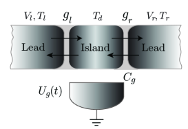
Figure 1: The sketch of a SET device. The leads are kept at different temperatures (chemical potentials) inducing heat (electric) currents.

AES-approach has well-known limitations. Deriving AES action one assumes that the products of electron Green’s functions averaged over disorder are substituted with products of disorder-averaged Green’s functions in every calculation. That is why the processes of phase-coherent multiple impurity scattering inside the island are left out. The limitations in the regime $g\gg 1$ and $g\ll 1$ were discussed in detail in Refs. [efetov-bel, ] and  [Efetov-Tschersich, ], respectively. It was shown that at temperatures $T\gg\max\{1,g\}\delta$, AES-action approach is justified. Following Ref. [AltlandMeyer, ], we shall term the temperature range, $\max\{1,g\}E_{c}\gg T\gg\max\{1,g\}\delta$ as an interaction without coherence regime. This ‘interaction without coherence’ regime is an attainable experimental reality, e.g. in experiments reported in Refs. [Dzurak, ] and [Scheibner, ] the necesary conditions were satisfied.

In the case of strong Coulomb blockade ($g\ll 1$), the theoretical study of relaxation of an electron distribution in the interaction without coherence regime has been done before for a single quantum dot [beloborodov4, ] and for an 1D array of quantum dots [beloborodov-glatz, ]. However, the considerations of Ref. [beloborodov4, ] have been restricted by assumptions that i) the electron distribution is the Fermi function with some temperature different from the equilibrium one; ii) transport is dominated by co-tunneling processes (Coulomb valley regime); iii) temperatures of the island and the reservoirs are close to each other.

In the present paper, we undertake the analysis of relaxation of an electron distribution function which is free of above-mentioned restrictions.

Since we are going to capture non-equlibrium physics, we employ the formalism of AES-action in its out-of-equilibrium form throughout the paper. We supplement it with quantum kinetic equation to explore relaxation dynamics of electron distribution. For a SET with large number of tunneling channels we derive the quantum kinetic equation with the collision integral due to escape of electrons to the reservoirs. It is valid in the entire span of values of $g$ and generalizes the one obtained in Ref.[BaskoKravtsov, ] for sequential tunneling (first order in $g$) and cotunneling (second order in $g$) approximations in the framework of the orthodox theory of the Coulomb blockade. In fact, our collision integral is always an infinite series in powers of $g$. Indeed, each tunneling event is accompanied by the radiation of a plasmon. That is why the collision integral becomes of the infinite order in the distribution function of electrons inside the island. This situation is entirely different from the one in Fermi liquid and leads to non-trivial relaxation.

As a test of the quantum kinetic equation, in the regime of linear response we derive analytical expressions for transport coefficients: conductance, thermal conductance and the response of electric current to temperature difference. In the regime of weak Coulomb blockade ($g\gg 1$) we establish the following new results for the transport coefficients: i) the conductance and thermal conductance violate Wiedemann-Franz law, and deviation of the Lorentz ratio $\mathcal{L}$ from value $\pi^{2}/3e^{2}$ demonstrates weak periodic dependence on the gate voltage; ii) the thermopower weakly oscillates with the gate voltage around zero value. Weak oscillations of the Lorentz ratio and thermopower with the gate voltage found in the regime $g\gg 1$ are manifestation of the known gate-voltage dependence of these quantities Amman ; BeenakkerStaring ; AndreevMatveev ; TurekMatveev ; MatveevAndreev1 ; kubala1 ; Nakanishi ; Zianni ; kubala2 in the strong Coulomb blockade regime, $g\ll 1$.

In weak and strong Coulomb blockade regimes we have employed the quantum kinetic equation to solve the relaxation of the electron distribution in two cases: i) the distribution of electrons inside the island is the Fermi-function with some temperature; ii) the distribution function of electrons inside the island is arbitrary. In the former case we have managed to extract the relaxation dynamics of the electron temperature; in the latter case we have obtained evolution of a distribution function itself. In both cases we assumed that electron escape to reservoirs is the primary relaxation mechanism. In general, the collision integral in the quantum kinetic equation is non-local in energy due to inelastic nature of tunneling processes: the radiation of plasmon always accompanies the tunneling event. In a number of wide parametric regimes: weak Coulomb blockade and Coulomb peak in the strong Coulomb blockade, the kernel of the quantum kinetic equation acquires a quasi-elastic form. However, the collision integral remains non-local in energy due to renormalization effects in these cases. The co-tunneling regime is qualitatively different: the kernel of the collision integral is entirely inelastic.

Our new result is that despite quasi-elastic form of the collision integral, strong Coulomb interaction dramatically changes the relaxation laws comparing to simple exponential ones expected from golden-rule type arguments. They suggest that electron relaxation rate is to be proportional to the width of electrons’ levels inside the island, $g\delta$, prompting simple exponential relaxation. The renormalization effects due to Coulomb interaction make the width of electrons’ levels dependent on the electron distribution and lead to the non-exponential relaxation laws. For example, in the regime of the sequential tunneling, we have discovered that there is a time regime in which relaxation of the electron temperature in a SET island is independent of the tunneling conductance $g$.

The paper is organized as follows. In Sec. II we introduce the hamiltonian and essential parameters of the problem. Sec. III is devoted to the out-of-equilibrium AES-model and to derivation of the quantum kinetic equation. Sec. IV is devoted to derivation of general expressions for the linear response coefficients. The relaxation dynamics of electrons in the island is explored in the weak ($g\gg 1$) and strong ($g\ll 1$) Coulomb blockade regimes in Sec. V-VI. Discussion of the results, comparision with other relaxation mechanisms, different from electron escape to reservoirs and conclusions are presented in Sec. VII.

II Formalism

A SET is described by the Hamiltonian

$$H=H_{0}+H_{c}+H_{t},$$ (1)

where

$$H_{0}=\sum_{k,i}\varepsilon^{(i)}_{k}a^{(i)\dagger}_{k}a^{(i)}_{k}+\sum_{\alpha}\varepsilon^{(d)}_{\alpha}d^{\dagger}_{\alpha}d_{\alpha}.$$ (2)

describes free electrons in the leads and the island, $H_{c}$ describes Coulomb interaction of carriers in the island, and $H_{t}$ describes the tunneling. Here operators $a^{(i){\dagger}}_{k}$ ($d^{\dagger}_{\alpha}$) create a carrier in the $i$-th lead (island). Then, the tunneling hamiltonian is

$$H_{t}=\sum_{k,\alpha,i}t^{(i)}_{k\alpha}a_{k}^{(i)\dagger}d_{\alpha}+{\rm H.c.}$$ (3)

The charging Hamiltonian of electrons in the box is taken in the capacitive form:

$$H_{c}=E_{c}\big{(}\hat{n}_{d}-q\big{)}^{2}.$$ (4)

Here $E_{c}=e^{2}/(2C)$ denotes the charging energy, and $\hat{n}_{d}$ is an operator of a particle number in the island:

$$\begin{split}\hat{n}_{d}=\sum_{\alpha}d^{\dagger}_{\alpha}d_{\alpha}.\end{split}$$ (5)

To characterize the tunneling it is convenient to introduce the following hermitean matrices:

$$\hat{g}^{(i)}_{kk^{\prime}}=(2\pi)^{2}\left[\delta(\varepsilon^{(i)}_{k})\delta(\varepsilon^{(i)}_{k^{\prime}})\right]^{1/2}\sum_{\alpha}t_{k\alpha}\delta(\varepsilon^{(d)}_{\alpha})t^{\dagger}_{\alpha k^{\prime}},$$ (6)

$$\check{{g}}^{(i)}_{\alpha\alpha^{\prime}}=(2\pi)^{2}\left[\delta(\varepsilon^{(d)}_{\alpha})\delta(\varepsilon^{(d)}_{\alpha^{\prime}})\right]^{1/2}\sum_{k}t^{\dagger}_{\alpha k}\delta(\varepsilon^{(i)}_{k})t_{k\alpha^{\prime}},$$ (7)

The first of them acting in the Hilbert space of the states of the lead, the second – in the space of the islands states. The energies $\varepsilon^{(i)}_{k},\varepsilon^{(d)}_{\alpha}$ are accounted from the Fermi level, and the delta-functions should be smoothed on the scale $\delta E$, such that $\max\{\delta,\delta^{(l,r)}\}\ll\delta E\ll T$. Here, $\delta$ and $\delta^{(l,r)}$ stand for mean level spacing of single-particle states on the island and reservoirs, respectively. The classical dimensionless conductance (in units $e^{2}/h$) of the junction between a reservoir and the island can be expressed as follows Glazman

$$g=g_{l}+g_{r},\qquad g_{l,r}=\sum_{k}\hat{g}^{(l,r)}_{kk}\equiv\sum_{\alpha}\check{g}^{(l,r)}_{\alpha\alpha}.$$ (8)

Therefore, each non-zero eigenvalue of $\hat{g}^{(i)}$ or $\check{g}^{(i)}$ corresponds to the transmittance of some ‘transport’ channel between a reservoir and the island. landauer The effective number of these ‘transport’ channels ($N^{(i)}_{\rm ch}$) is given by

$$N^{(i)}_{\rm ch}=\frac{\left(\sum\limits_{k}\hat{g}^{(i)}_{kk}\right)^{2}}{\sum\limits_{kk^{\prime}}\hat{g}^{(i)}_{kk^{\prime}}\hat{g}^{(i)}_{k^{\prime}k}}\equiv\frac{\left(\sum\limits_{\alpha}\check{g}^{(i)}_{\alpha\alpha}\right)^{2}}{\sum\limits_{\alpha\alpha^{\prime}}\hat{g}^{(i)}_{\alpha\alpha^{\prime}}\hat{g}^{(i)}_{\alpha^{\prime}\alpha}}.$$ (9)

The effective dimensionless conductance $g^{(i)}_{\rm ch}$ of a ‘transport’ channel can be written as follows

$$g^{(i)}_{\rm ch}=\frac{\sum\limits_{kk^{\prime}}\hat{g}^{(i)}_{kk^{\prime}}\hat{g}^{(i)}_{k^{\prime}k}}{\sum\limits_{k}\hat{g}^{(i)}_{kk}}\equiv\frac{\sum\limits_{\alpha\alpha^{\prime}}\hat{g}^{(i)}_{\alpha\alpha^{\prime}}\hat{g}^{(i)}_{\alpha^{\prime}\alpha}}{\sum\limits_{\alpha}\check{g}^{(i)}_{\alpha\alpha}}.$$ (10)

The dimensionless conductance $g$ then becomes

$$g=g_{l}+g_{r},\qquad g_{l,r}=g^{(l,r)}_{\rm ch}N^{(l,r)}_{\rm ch}.$$ (11)

In what follows we will always assume

$$g^{(i)}_{\rm ch}\ll 1,\qquad N^{(i)}_{\rm ch}\gg 1.$$ (12)

Notice that under these circumstances the conductances $g_{l,r}$ can still be large provided the effective number of channels $N^{(l,r)}_{\rm ch}$ is sufficiently large.

III Action and kinetic equaitons

III.1 AES-action

To tackle the system which is out of equilibrium we have to employ essentially non-equilibrium formalism. Keldysh technique is thus the only way through. We employ Keldysh form of AES-action (we sketch the known details of derivation in Appendix A): zaikin ; Skvortsov

$$S=S_{c}+S_{d}$$ (13)

where

$$S_{c}=\frac{1}{E_{c}}\int\dot{\varphi_{c}}\dot{\varphi_{q}}dt+2q\int\dot{\varphi}_{q}dt.$$ (14)

Here $\varphi_{c,q}=(\varphi_{+}\pm\varphi_{-})/2$ with $\varphi_{\pm}$ denoting bosonic field on both branches of Keldysh contour. Physically, the bosonic field is associated with the fluctuating electric potential on the island. In terms of classic and quantum boson exponents

$$X_{c,q}=\frac{1}{\sqrt{2}}\big{(}e^{i\varphi_{+}}\pm e^{i\varphi_{-}}\big{)},$$ (15)

the dissipative part of AES-action reads:

$$\begin{split}S_{d}&=\frac{g}{4}\int\Big{(}\bar{X}_{c}(t)\bar{X}_{q}(t)\Big{)}\\ &\times\begin{pmatrix}0&\Pi^{A}(t,t^{\prime})\\ \Pi^{R}(t,t^{\prime})&\ \Pi^{K}(t,t^{\prime})\end{pmatrix}\begin{pmatrix}X_{c}(t^{\prime})\\ X_{q}(t^{\prime})\end{pmatrix}dtdt^{\prime}.\end{split}$$ (16)

Here $\Pi^{R,A,K}$ are corresponding components of electron polarization operator in the Keldysh space. They are given by a standard formulae presented for reference in Appendix A. In a case of constant density of states (DOS) in the island and leads the kernel of the AES action can be simplified:

$$\Pi^{R,A,K}(t,t^{\prime})=\int\frac{d\omega}{2\pi}\Pi^{R,A,K}_{\omega}(\tau)e^{-i\omega(t-t^{\prime})},$$ (17)

$$\Pi^{R,A}_{\omega}(\tau)=\mp i\sum_{\alpha}\frac{g_{\alpha}}{g}\int\big{[}F^{d}_{\varepsilon}(\tau)-F^{\alpha}_{\varepsilon-\omega}(\tau)\big{]}\frac{d\varepsilon}{2\pi},$$ (18)

$$\Pi^{K}_{\omega}(\tau)=2i\sum_{\alpha}\frac{g_{\alpha}}{g}\int(1-F^{d}_{\varepsilon}(\tau)F^{\alpha}_{\varepsilon-\omega}(\tau))\frac{d\varepsilon}{2\pi}.$$ (19)

Here we define a slow time $\tau=(t+t^{\prime})/2$. Function $F_{\varepsilon}(\tau)$ is given in terms of the Wigner transform $f_{\varepsilon}(\tau)$ of the electron distribution function $f(t,t^{\prime})$: $F_{\varepsilon}(\tau)=1-2f_{\varepsilon}(\tau)$. $\Pi^{R,A,K}_{\omega}(\tau)$ are Wigner transforms of corresponding functions in time domain.

As seen from the structure of the r.h.s. of (19), it is suitable to introduce function $F^{r}_{\varepsilon}=(\sum_{\alpha}g_{\alpha}F^{\alpha}_{\varepsilon})/g$ which may be called the effective distribution function of two reservoirs. It is that combination of reservoir distribution functions that enters all the following equations of the paper.

Although Eq. (18) is exact we neglect all derivatives with respect to slow time $\tau$ in Eq. (19). It is also convenient to introduce function $B_{\omega}(\tau)$ in accordance with

$$\Pi^{K}_{\omega}(\tau)=2i\operatorname{Im}\Pi^{R}_{\omega}(\tau)B_{\omega}(\tau)$$ (20)

relating Keldysh and retarded (advanced) components of polarization operator. The function $B_{\omega}(\tau)$ plays a role of a distributiion function for electron-hole excitations. In the equilibrium it is given by $\coth(\omega/2T)$.

In what follows we assume that electrons in the leads are locally thermalized such that $f_{\varepsilon}^{l,r}(\tau)$ are the Fermi-functions. Depending on the parameters of the model, both quasi-equilibrium and non-equilibrium regimes can exist in the island. Therefore, we assume $F_{\varepsilon}^{d}(\tau)$ to be an arbitrary function slow varying with time $\tau$, and derive the kinetic equation for $F_{\varepsilon}^{d}(\tau)$ by which the AES action should be supplemented.

III.2 Kinetic equations

The starting point for deriving kinetic equation for a SET is the Dyson equation for the Keldysh component of electron’s Green’s function: KEStandard

$$(\partial_{t}+\partial_{t^{\prime}})F^{d}(t,t^{\prime})=\frac{i}{4\pi^{2}\nu_{d}}\Bigl{[}\Sigma^{K}-\Sigma^{R}\cdot F^{d}+F^{d}\cdot\Sigma^{A}\Bigr{]}_{t,t^{\prime}}.$$ (21)

Here, $\nu_{d}=\delta^{-1}=\overline{\sum_{\alpha}\delta(\varepsilon^{d}_{\alpha})}$ is an averaged single particle density of states in the island and $\Sigma^{K,R,A}$ are the components of self-energy in Keldysh space. To the second-order in tunneling Hamiltonian $H_{T}$ (lowest order in $1/N_{\rm ch}$) the Wigner transform of the self-energy shown in Fig. 2a reads (see Appendix B)

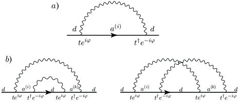
Figure 2: Feynman diagrams for fermion self-energy: a) second order in $H_{T}$; b) fourth order in $H_{T}$.

$$\Sigma^{R,A}_{\varepsilon}(\tau)=\pm\frac{\pi g}{2}\int\frac{d\omega}{2\pi}\Bigl{[}{\cal D}^{K}_{\omega}(\tau)\pm 2F^{r}_{\varepsilon-\omega}(\tau){\cal D}^{R,A}_{\omega}(\tau)\Bigr{]},$$

$$\Sigma^{K}_{\varepsilon}(\tau)=\pi g\int\frac{d\omega}{2\pi}\Bigl{[}F^{r}_{\varepsilon-\omega}(\tau){\cal D}^{K}_{\omega}(\tau)+2i\operatorname{Im}{\cal D}^{R}_{\omega}(\tau)\Bigr{]}.$$ (22)

Here we perform Wigner transform of the exact sel-energies and introduce the correlation functions of boson exponents:

$$\begin{split}{\cal D}^{R}(t,t^{\prime})&=-i\langle X_{c}(t)\bar{X}_{q}(t^{\prime})\rangle,\\ {\cal D}^{A}(t,t^{\prime})&=-i\langle X_{q}(t)\bar{X}_{c}(t^{\prime})\rangle,\\ {\cal D}^{K}(t,t^{\prime})&=-i\langle X_{c}(t)\bar{X}_{c}(t^{\prime})\rangle.\end{split}$$ (23)

It is convenient to parametrize ${\cal D}^{K}(t,t^{\prime})$ via the boson distribution function $\mathcal{B}(t,t^{\prime})$:

$${\cal D}^{K}_{t,t^{\prime}}=\Big{(}{\cal D}^{R}\cdot{\cal B}-{\cal B}\cdot{\cal D}^{A}\Big{)}_{t,t^{\prime}}.$$ (24)

It is worthwhile to mention that the next ( fourth order in $H_{T}$) contribution to the self-energy which is shown in Fig. 2b is of the order $g^{2}/N_{ch}$. This correction to the self-energy is of the same order as terms omitted in the course of derivation of the AES action (16). In the considered limit $N_{ch}\gg 1$ it can be safely neglected.

Performing Wigner transform of Eq. (21) and neglecting all slow time derivatives in its r.h.s. we obtain the quantum kinetic equation for the distribution function of electrons on the island of a SET:

$$\begin{split}&\partial_{\tau}F^{d}_{\varepsilon}(\tau)=-\sum_{\alpha=l,r}\frac{g_{\alpha}}{2\pi\nu_{d}}\int\frac{d\omega}{2\pi}\,\textrm{Im}\,{\cal D}^{R}_{\omega}(\tau)\\ &\times\Bigl{\{}\Bigl{(}F^{\alpha}_{\varepsilon-\omega}(\tau)-F^{d}_{\varepsilon}(\tau)\Bigr{)}{\cal B}_{\omega}(\tau)+1-F^{d}_{\varepsilon}(\tau)F^{\alpha}_{\varepsilon-\omega}(\tau)\Bigr{\}}.\end{split}$$ (25)

This quantum kinetic equation constitutes one of the main results of the present paper. It describes evolution of the distribution function $F_{\varepsilon}^{d}(\tau)$ of electrons in the island due to interaction with boson field $\varphi$ and tunneling to the leads and back. The quantum kinetic equation (25) is derived for any values of $g_{r}$ and $g_{l}$; the r.h.s. of Eq. (25) can be written as the series in powers of $g$ due to the presence of $\,\textrm{Im}\,{\cal D}_{\omega}^{R}(\tau)$ and ${\cal B}_{\omega}$. The boson distribution ${\cal B}_{\omega}$ is determined by electron distribution function $F_{\varepsilon}^{d}(\tau)$ and should be found from the solution of the AES-action (13).

At $g\gg 1$ the kernel ($\,\textrm{Im}\,{\cal D}^{R}_{\omega}$) of the collision integral of the quantum kinetic equation (25) resembles the kernel of the collision integral in the quantum kinetic equation for disordered electron liquid Schmid ; AA ; AA1 for energy transfers $\omega\gg g\delta$ as it is expected. efetov-bel At $g\ll 1$ the quantum kinetic equation (25) which takes into account the renormalization effects via $\,\textrm{Im}\,{\cal D}^{R}_{\omega}$ generalizes the kinetic equation derived in Ref. [BaskoKravtsov, ] in the framework of the orthodox theory kulik for sequential tunneling and inelastic cotunneling approximations.

IV Transport coefficients

Using quantum kinetic equation (25) we are able to derive general formulae for all linear response coefficients of the SET for any value of $g$. Voltage $(\Delta V=V_{r}-V_{l})$ and temperature $(\Delta T=T_{r}-T_{l})$ differences across the SET cause charge $(I^{(e)})$ and heat $(I^{(q)})$ currents. Electric and thermoelectric transport coefficients are defined as

$$\begin{pmatrix}I^{(e)}\\ I^{(q)}\end{pmatrix}=\begin{pmatrix}G_{V}&G_{T}\\ M&K\end{pmatrix}\begin{pmatrix}\Delta V\\ \Delta T\end{pmatrix}.$$ (26)

Here coefficients $M$ and $G_{T}$ (the response of a heat current to voltage difference and the response of electric current to temperature difference, respectively) are related via Onsager relation $M=G_{T}T$. Abrikosov The thermal conductance $\kappa$ is usually defined as $\kappa=K-G_{V}TS^{2}$ where $S=G_{T}/G_{V}$ stands for the thermopower. The electric and heat currents in the $\alpha$-th reservoir can be found as

$${}\,\begin{pmatrix}I^{(e)}_{\alpha}\\ I^{(q)}_{\alpha}\end{pmatrix}=-\frac{g_{\alpha}}{4\pi}\int d\varepsilon\begin{pmatrix}1\\ \varepsilon\end{pmatrix}\int\frac{d\omega}{2\pi}\,\textrm{Im}\,{\cal D}^{R}_{\omega}(\tau)$$ (27)

$$\times\Bigl{\{}\Bigl{(}F^{d}_{\varepsilon+\omega}(\tau)-F^{\alpha}_{\varepsilon}(\tau)\Bigr{)}{\cal B}_{\omega}(\tau)-1+F^{\alpha}_{\varepsilon}(\tau)F^{d}_{\varepsilon+\omega}(\tau)\Bigr{\}}.$$

The current conservation corresponds to the condition $I^{e}_{l}+I^{e}_{r}=0$. It fixes the boson distribution function ${\cal B}_{\omega}$ to be equal to the electron-hole distribution function $B_{\omega}$ introduced in Eq. (20):

$$B_{\omega}(\tau) = \frac{\Pi_{\omega}^{K}(\tau)}{2i\,\textrm{Im}\,\Pi_{\omega}^{R}(\tau)}$$ (28)

$$= \frac{\sum\limits_{\alpha=l,r}g_{\alpha}\int d\varepsilon\Bigl{[}1-F^{d}_{\varepsilon}(\tau)F^{\alpha}_{\varepsilon-\omega}(\tau)\Bigr{]}}{\sum\limits_{\alpha=l,r}g_{\alpha}\int d\varepsilon\Bigl{[}F^{d}_{\varepsilon}(\tau)-F^{\alpha}_{\varepsilon-\omega}(\tau)\Bigr{]}}.$$

The heat current conservation $I^{q}_{l}+I^{q}_{r}=0$ determines the equilibrium temperature of the island:

$$T^{\rm(eq)}_{d}=\frac{g_{l}T_{l}+g_{r}T_{r}}{g_{l}+g_{r}}.$$ (29)

A straightforward computation of charge and heat currents gives

$$\begin{split}\begin{pmatrix}I^{(e)}_{l}\\ I^{(q)}_{l}\end{pmatrix}&=-\frac{g_{l}g_{r}}{g}\frac{e}{4\pi}\int\frac{d\omega}{2\pi}\frac{\operatorname{Im}{\cal D^{R}_{\omega}}}{\sinh^{2}\frac{\beta\omega}{2}}\\ &\times\begin{pmatrix}\beta\omega&-\frac{(\beta\omega)^{2}}{2}\\ -\frac{\beta\omega^{2}}{2}&\omega\frac{\pi^{2}+(\beta\omega)^{2}}{3}\end{pmatrix}\begin{pmatrix}e\Delta V\\ \Delta T\end{pmatrix}.\end{split}$$ (30)

Introducing the quantities $g^{\prime},g_{T}^{\prime}$, and $k^{\prime}$ as

$$\begin{split}\begin{pmatrix}G_{V}&G_{T}\\ M&K\end{pmatrix}&=\frac{e^{2}}{h}\frac{g_{l}g_{r}}{(g_{l}+g_{r})^{2}}\begin{pmatrix}g^{\prime}&-\frac{1}{e}g_{T}^{\prime}\\ -\frac{T}{e}g_{T}^{\prime}&\frac{T}{e^{2}}k^{\prime}\end{pmatrix},\end{split}$$ (31)

we obtain

$$\begin{pmatrix}g^{\prime}\\ g_{T}^{\prime}\\ k^{\prime}\end{pmatrix}=-g\int\frac{d\omega}{4\pi}\frac{\operatorname{Im}{\cal D^{R}_{\omega}}}{\sinh^{2}\frac{\beta\omega}{2}}\beta\omega\begin{pmatrix}1\\ \frac{\beta\omega}{2}\\ \frac{\pi^{2}+(\beta\omega)^{2}}{3}\end{pmatrix}.$$ (32)

We stress that Eq. (32) is valid for any value of tunneling conductance $g$. It generalizes expressions for transport coefficients obtained in Refs. [schoeller, ; kubala2, ] for $g\ll 1$ to arbitrary values of $g$.

It is worthwhile to express Eq. (32) in terms of the tunneling density of states of electrons in the island (see Appendix C):

$$\nu_{d}(\varepsilon)=-\nu_{d}\int\,\textrm{Im}\,{\cal D}^{R}_{\omega}\Bigl{\{}\coth\frac{\omega}{2T}-\tanh\frac{\varepsilon+\omega}{2T}\Bigr{\}}\frac{d\omega}{2\pi}.$$ (33)

Substituting expression (33) for the tunneling density of states and performing standard integrals with Fermi and Bose distribution functions one can check that the results (32) are allowed to be exactly rewritten in the form

$$\begin{pmatrix}g^{\prime}\\ g_{T}^{\prime}\\ k^{\prime}\end{pmatrix}=g\int d\varepsilon\frac{\nu_{d}(\varepsilon)}{\nu_{d}}\bigg{(}-\frac{\partial f_{\varepsilon}^{d}}{\partial\varepsilon}\bigg{)}\begin{pmatrix}1\\ \varepsilon\\ \varepsilon^{2}\end{pmatrix}.$$ (34)

Eq. (34) for the transport coefficients resembles the corresponding expression in the Fermi-liquid. AGD ; Abrikosov However, contrary to Fermi-liquid, the tunneling density of states $\nu_{d}(\varepsilon)$ has strong dependence on energy for $\varepsilon\to 0$. In general, $\nu_{d}(\varepsilon)=\nu_{d}^{\rm even}(\varepsilon)+\nu_{d}^{\rm odd}(\varepsilon)$ where $\nu_{d}^{\rm even/odd}(\varepsilon)$ is even/odd function of $\varepsilon$. It can be shown that $\nu_{d}^{\rm even/odd}(\varepsilon)$ is even/odd function of the external charge $q$. Therefore, $g^{\prime}$ and $k^{\prime}$ are even functions of $q$ whereas $g_{T}^{\prime}$ is an odd function of the external charge.

For macroscopic samples of ordinary metals, the Wiedemann-Franz law provides a universal relation between the conductance and thermal conductance. It states that the Lorenz ratio $\mathcal{L}=\kappa/(G_{V}T)$ , is a constant given by the Lorenz number $\pi^{2}/3e^{2}$. As follows from Eq. (34), one can expect the violation of Wiedemann-Franz law in the presence of strong dependence of $\nu_{d}(\varepsilon)$ on electron energy.

In the case $g\gg 1$ one is able to perform perturbative expansion in $1/g$ and take into account non-perturbative corrections. The function $\,\textrm{Im}\,{\cal D}_{\omega}^{R}$ acquires the following form in the equilibrium burmistrov2

$$\,\textrm{Im}\,{\cal D}^{R}_{\omega}=-\frac{\pi}{T}\left[1-\frac{2}{g}\ln\frac{gE_{c}e^{\gamma}}{2\pi^{2}T}-\frac{g^{2}E_{c}}{\pi^{2}T}e^{-g/2}\cos 2\pi q\right]\omega\delta(\omega)$$

$$-\frac{2\pi}{g\omega}\left[1+\frac{g^{3}E_{c}}{2\pi^{2}T}e^{-g/2}\cos 2\pi q\right]$$

$$+\frac{g^{2}E_{c}}{\pi T}e^{-g/2}\cos 2\pi q\frac{\omega}{\omega^{2}+4\pi^{2}T^{2}}$$

$$-\frac{g^{2}E_{c}}{T}e^{-g/2}\sin 2\pi q\left(\delta(\omega)-\frac{2T}{\omega^{2}+4\pi^{2}T^{2}}\right).$$ (35)

Here, function $\omega\delta(\omega)$ can be understood as $\,\textrm{Im}\,a/[\pi(\omega+a+i0)]$ where the limit $a\to 0$ should be performed at the very end of all calculations, (this calculation can be, e.g. integration over $\omega$). The non-perturbative in $1/g$ corrections (exponential terms $\exp(-g/2)$) come from Korshunov instantons korshunov of the AES-action. Then by using Eq. (35) we find from Eq. (32)

$$g^{\prime}=g-2\ln\frac{gE_{c}}{T}-\frac{g^{3}E_{c}}{6T}e^{-g/2}\cos 2\pi q,$$ (36)

$$g^{\prime}_{T}=-\frac{2g^{3}E_{c}}{\pi T}e^{-g/2}\Big{(}1-\frac{\pi^{2}}{12}\Big{)}\sin 2\pi q,$$ (37)

$$k^{\prime}=\frac{\pi^{2}}{3}\Big{(}g^{\prime}+\frac{4}{3}+\frac{2g^{3}E_{c}}{\pi^{2}T}\cos 2\pi q\Big{[}\frac{\pi^{2}}{3}-3\Big{]}\Big{)}.$$ (38)

The result for $g^{\prime}$ has been obtained in Ref. [AltlandMeyer, ]. Equations (37)-(38) are new and valid for temperatures $T\gg g^{2}E_{c}\exp(-g/2)$. We emphasize that $g_{T}^{\prime}$ has only non-perturbative instanton) contribution. The same holds for the thermopower:

$$S=-\frac{2g^{2}E_{c}}{\pi eT}\left(1-\frac{\pi^{2}}{12}\right)\exp\left(-\frac{g}{2}\right)\sin 2\pi q.$$ (39)

At $g\gg 1$ the violation of the Wiedemann-Franz law is weak and the Lorentz number is given as

$$\mathcal{L}=\frac{\pi^{2}}{3e^{2}}\Biggl{[}1+\frac{4}{3g}+\frac{2}{3}\left(1-\frac{9}{\pi^{2}}\right)\frac{g^{2}E_{c}}{T}e^{-g/2}\cos 2\pi q\Biggr{]}.$$ (40)

Due to the presence of the non-perturbative contribution, the Lorentz number is temperature dependent and oscillates as a function of the external charge $q$. Eqs. (39) and (40) constitute one of the main results of the present paper.

In the strong coupling regime $g\ll 1$, Eq. (32) supplemented by the proper expression for $\,\textrm{Im}\,{\cal D}^{R}_{\omega}$ (cf. Eqs. (75) and (114)) results in exactly the same expressions for the transport coefficients as obtained in Refs. [schoeller, ; kubala1, ; kubala2, ; Zianni, ]. We refer a reader to these works for details.

V Relaxation of electrons in the island, weak coupling regime $g\gg 1$

Next, we want to illustrate the ability of quantum kinetic equation (25) combined with fine field-theoretical scaling of essential physical quantities. We consider the problem of relaxation of electrons in the island towards the equilibrium due to the tunneling to the reservoirs and back. There are two possible scenarios. The first one can be refered to as a quasi-equilibrium regime. The electron distribution inside the island is given by the Fermi-function but with non-equilibrium temperature $T_{d}$ which slowly relaxes to its equilibrium value. The second scenario is fully non-equilibrium regime when electron distribution is arbitrary. Which scenario persists depends on the ratio $\tau_{E}/\tau_{ee}$ where $\tau_{E}$ stands for the energy relaxation time due to tunneling mechanism and $\tau_{ee}$ for the energy relaxation time due to electron-electron interaction in the island. The non-equilibrium regime persists provided $\tau_{E}\ll\tau_{ee}$ and the quasi-equilibrium regime is possible if $\tau_{E}\gg\tau_{ee}$. We will argue below (see Sec. VII) that both scenarios are possible.

There is one more relaxation time involved: $\tau_{RC}$ which determines relaxation of the electric charge on the island. In the weak Coulomb blockade regime, $\tau_{RC}$ is given by the following clasical estimate: $\tau_{RC}\simeq 2\pi/gE_{c}$. As we shall see below, $\tau_{E}\gg\tau_{RC}$. Therefore, it is allowed to assume that at first there is quick relaxation of the electric charge on the island and, then, slow relaxation of the electron distribution function or temperature towards the equilibrium. Technically, it means that initial electron distribution function $F_{\varepsilon}^{d}(0)$ satisfies the constraint $\int d\varepsilon[F_{\varepsilon}^{d}(0)-F_{\varepsilon}^{r}]=0$.

As was discussed in the Introduction, the renormalization of physical observables drastically changes the relaxation dynamics of the system. Therefore, before solving kinetic equation we need to establish the scaling of a theory’s coupling constants under non-equilibrium conditions.

V.1 Renormalization of AES-action at $g\gg 1$

The AES-action is renormalized due to its nonlinear form. In the equilibrium case renormalization of the action is well-known (see e.g., Ref. [zaikin, ]). In our case non-equilibrium makes the problem non-trivial. As in equilibrium, we expect the necessary scaling of the coupling constant $g$. The additional question that inevitably arises is whether the structure of the kernel of AES action (the components of polarization operator $\Pi_{\omega}$ in Keldysh space in Eq. (16)) is changed due to renormalization? The details of the calculation are presented in Appendix D. We prove that the structure of the bare action is fully restored, the kernel of the AES action being intact during renormalization group (RG) procedure. The coupling constant renormalizes according to

$$g(\underline{\Lambda})=g(\overline{\Lambda})-2\int^{\overline{\Lambda}}_{\omega=\underline{\Lambda}}\frac{B_{\omega}(\tau)}{\omega}d\omega.$$ (41)

Here high energy scale $\overline{\Lambda}$ is naturally set by the first term in Eq. (14): $\overline{\Lambda}\sim gE_{c}$. To demonstrate that the integral in Eq. (41) is indeed logarithmic we explore the behavior of the integrand at $\omega\rightarrow\infty$. It is straightforward to get the following asymptotic for function $B_{\omega}$ at $\omega\to\infty$:

$$\begin{split}B_{\omega}&=\operatorname{sgn}\omega+\delta B_{\omega},\\ \delta B_{\omega}&=(F^{d}_{\omega}-\operatorname{sgn}\omega)\\ &+\frac{1}{2\omega}\sum_{\alpha}\frac{g_{\alpha}}{g}\int(\varepsilon+\omega)\big{(}F^{d}_{\varepsilon+\omega}-F^{d}_{\omega}\big{)}\partial_{\varepsilon}F^{\alpha}_{\varepsilon}d\varepsilon.\end{split}$$ (42)

We expect that any physical distribution function obeys the condition $F^{d}_{\varepsilon}\rightarrow\operatorname{sgn}\,\varepsilon$ at $\varepsilon\rightarrow\infty$. Then

$$\lim_{\omega\rightarrow\infty}\delta B_{\omega}=0.$$ (43)

Therefore, the high-energy asymptotic of function $B_{\omega}$ is given by $\operatorname{sgn}\varepsilon$ as in the equilibrium. This way, the logarithmic behavior of integral in Eq. (41) is ascertained.

To get the renormalized action one has to integrate out all the frequencies down to the lowest scale $\omega_{0}$, at which the RG stops.This energy scale can be determined as

$$\delta B(\omega_{0})\sim 1.$$ (44)

Let $\varepsilon_{d}$ be a characteristic energy scale of the island distribution function (the scale at which electron distribution function $F^{d}_{\varepsilon}$ becomes almost equal to $\operatorname{sgn}\varepsilon$). Then one can easily check that the following estimate holds (see Appendix D for elaborate details)

$$\omega_{0}\sim\max\{\varepsilon_{d},T_{r},T_{l}\},$$ (45)

where $T_{r},T_{l}$ are temperatures of the reservoirs. Energy scale $\omega_{0}$ serves as a natural lower cut-off, $\underline{\Lambda}=\omega_{0}$, in the RG procedure. Finally, we find

$$g(\omega_{0})=g-2\ln\frac{gE_{c}}{\omega_{0}}.$$ (46)

In the equilibrium, $\varepsilon_{d}=T_{r}=T_{l}=T$ and one finds $\omega_{0}=T$. Eqs. (45)-(46) describe renormalization of the AES-action under non-equilibrium conditions.

V.2 Non-equilibrium regime

The relaxation problem is formulated as follows. At $t=0$ the island is heated and some electron distribution function $F_{\varepsilon}^{d}(0)$ is created. The characteristic energy $\varepsilon_{d}$ of electrons in the island is larger than temperatures of the reservoirs, which are kept fixed and equal to each other $\varepsilon_{d}>T_{r}=T_{l}$. The system is released and the island is cooling down due to the tunneling of electrons to the reservoirs and back.

Performing expansion to the second order in boson fields $\varphi_{c,q}$, one straightforwardly finds (see Appendix D)

$$\operatorname{Im}{\cal D}^{R}_{\omega}=-\frac{2\pi\delta(\omega)}{B_{\omega}}\Big{(}1-\frac{1}{g}\int\frac{B_{\omega}}{\omega}d\omega\Big{)}-\frac{2\pi}{g\omega}.$$ (47)

We mention that this result generalizes the perturbative (independent of $q$) part of Eq. (35) to the non-equilibrium case. With the help of (47) one can compute the collision integral in the r.h.s. of the quantum kinetic equation (25) and obtain

$$\begin{split}\partial_{\tau}F_{\varepsilon}^{d}(\tau)&=-\frac{\mathcal{G}(\tau)\delta}{2\pi}(F^{d}_{\varepsilon}(\tau)-F^{r}_{\varepsilon}),\\ {\cal G}(\tau)&=g-\int\frac{B_{\omega}(\tau)}{\omega}\,d\omega.\end{split}$$ (48)

Here we neglect last term in Eq. (47) for the following reasons. It gives contribution of the order of unity whereas the first term in Eq. (47) involves $\int d\omega\,B_{\omega}/\omega\sim\ln gE_{c}/\varepsilon_{d}\gg 1$. Although, Eq. (48) has a quasi-elastic form, in fact, it is highly non-linear equation: $\mathcal{G}(\tau)$ involves information about the electron distribution at all energies.

As was shown above, the quantity ${\cal G}(\tau)$ has meaning of the renormalized coupling constant of the theory. Simple algebra leads us to the differential equation for the function $\mathcal{G}(\tau)$: Footnote1

$$\partial_{\tau}{\cal G}(\tau)=-\frac{\delta{\cal G}(\tau)}{2\pi}\Big{(}{\cal G}(\tau)-{\cal G}_{r}\Big{)},$$ (49)

$${\cal G}_{r}=g-\int\frac{d\omega}{\omega}\coth\frac{\omega}{2T_{r}}.$$

The solution reads

$${\cal G}(\tau)=\frac{\mathcal{G}(0)\mathcal{G}_{r}}{\mathcal{G}(0)+\big{(}\mathcal{G}_{r}-\mathcal{G}(0)\big{)}e^{-\frac{\mathcal{G}_{r}\delta}{2\pi}\tau}}.$$ (50)

Now by using this result we integrate Eq. (48) and obtain the evolution of the electron distribution function $F^{d}_{\varepsilon}$:

$$F^{d}_{\varepsilon}(\tau) = F_{\varepsilon}^{r}+\Bigl{(}F^{d}_{\varepsilon}(0)-F_{\varepsilon}^{r}\Bigr{)}$$ (51)

$$\times \left\{\frac{\mathcal{G}(0)}{\mathcal{G}_{r}}\left[\exp\left(\frac{\mathcal{G}_{r}\delta}{2\pi}\tau\right)-1\right]+1\right\}^{-1}.$$

Eq. (51) demonstrates energetically uniform relaxation of the electron distribution function. This fact is a direct consequence of the quasi-elastic form of the kinetic equation (48). However, due to renormalization effects the form of the relaxation law is different from the exponential one.

Let us define the characteristic energy $\varepsilon_{d}$ as $\varepsilon_{d}^{2}-T_{r}^{2}=(3/\pi^{2})\int d\varepsilon\,\varepsilon(F_{\varepsilon}^{r}-F_{\varepsilon}^{d})$ such that $\varepsilon_{d}=T_{d}$ in the quasi-equilibrium case $F_{\varepsilon}^{d}=\tanh(\varepsilon/2T_{d})$. Then, in the case $\varepsilon_{d}(0)\gg T_{r}$ and at not too long times $\tau\ll 2\pi/\delta\mathcal{G}_{r}$, one finds from Eq. (51) that the characteristic energy decreases according to the power-law:

$$\varepsilon_{d}(\tau)=\varepsilon_{d}(0)\left[1+\frac{\delta\mathcal{G}(0)}{2\pi}\tau\right]^{-1/2}.$$ (52)

V.3 Quasi-equilibrium regime

In the quasi-equilibrium regime, we need to take into account the collision integral $I^{(ee)}_{\varepsilon}$ due to electron-electron interaction in the island. AA ; Schmid As this term is added to the r.h.s. of Eq. (25), it makes the electron distribution $F_{\varepsilon}^{d}$ to be the Fermi-function. Multiplying both parts of Eq. (25) by $\varepsilon$ and integrating them over energy, we obtain the following equation (the well-known identity $\int d\varepsilon\,\varepsilon I^{(ee)}_{\varepsilon}=0$ is used):

$$\frac{dT^{2}_{d}}{d\tau}=-\frac{g\delta}{2\pi}(T_{d}^{2}-T_{r}^{2}).$$ (53)

Here we use the leading (classical) part of Eq. (47) ($\,\textrm{Im}\,\mathcal{D}^{R}_{\omega}=-2\pi\delta(\omega)/B_{\omega}$). Equation (53) yields standard exponential relaxation towards the equilibrium. In the limit $T_{d}\gg T_{r}$ ($\mathcal{G}(0)\gg\mathcal{G}_{r}$) it is also possible to compute collision integral using the entire one-loop expression (47) of its kernel. Naturally, one-loop correction reveals itself in the logarithmic renormalization of $g$ in the r.h.s. of Eq. (53). By using Eq. (47), we find

$$\begin{split}\frac{dT^{2}_{d}}{d\tau}&=-\frac{\mathcal{G}(\tau)\delta}{2\pi}T_{d}^{2},\\ {\cal G}(\tau)&=g-2\ln\frac{gE_{c}}{cT_{d}(\tau)}\end{split}$$ (54)

where $c$ is a numerical constant of the order of unity which does not influence final results. The solution of (54) reads:

$$\begin{split}T_{d}(\tau)&=T_{d}(0)\exp\bigg{(}-\frac{{\cal G}(0)}{2}\Big{[}1-e^{-\delta\tau/2\pi}\Big{]}\bigg{)}\\ \tau&\ll\frac{2\pi}{\delta}\ln\frac{\mathcal{G}(0)}{\mathcal{G}_{r}}.\end{split}$$ (55)

The condition in the second line of Eq. (55) implies that solution holds for not too long times at which $T_{d}(\tau)\gg T_{r}$ (${\cal G}(\tau)\gg{\cal G}_{r}$). The logarithmic renormalization of the conductance changes the character of temperature relaxation. At long times $2\pi/\delta\ll\tau\ll(2\pi/\delta)\ln\mathcal{G}(0)/\mathcal{G}_{r}$, the cooling of the island slows down in comparison to the standard exponential decay which is developed at short times $\tau\ll 2\pi/\delta$:

$$T_{d}(\tau)=T_{d}(0)e^{-\frac{{\cal G}(0)\delta\tau}{4\pi}}.$$ (56)

It is instructive to compare the relaxation of temperature in the quasi-equilibrium regime and the characteristic energy $\varepsilon_{d}$ in the non-equilibrium regime given by Eqs. (56) and (52) at times $\tau\ll 2\pi/\delta\mathcal{G}_{r}$, respectively. While the former demonstrates exponential behavior, the latter decreases in accordance with the power-law.

VI Relaxation of electrons in the island, strong coupling regime, $g\ll 1$

In the strong coupling regime there are two possible scenarios for relaxation of electrons in the island of the SET. The first one persists if $\tau_{E}\ll\tau_{ee}$. In this non-equilibrium case the carriers inside the island do not have time to thermalize and to form the Fermi-distribution with some temperature. In this case the the time evolution of distribution function itself becomes the main objective. This task is solved in section VI.3 below. The second scenario develops in the opposite limit, $\tau_{E}\gg\tau_{ee}$. Namely, the relaxation rate due to electron-electron interaction inside the island is much faster than the rate due to electron tunneling through the contacts. Thus, the temperature of carriers in the island becomes a well defined characteristic of a system. Consequently, the relaxation of the island’s temperature will be the focus of our analysis in section VI.4.

As in the previous section we shall assume that the electric charge on the island quickly relaxes and only then slow relaxation of the electron distribution or temperature starts. In the strong Coulomb blockade regime this picture is well justified since $1/\tau_{RC}\simeq g\max\{T,\Delta\}\gg 1/\tau_{E}$.

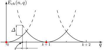
Figure 3: (Color online) Charging energy $E_{ch}=E_{c}(n-q)^{2}$ as a function of gate charge $q$.

We concentrate on the most interesting case: the vicinity of a degeneracy point: $q=k+1/2$ where $k$ is an integer. Following Ref. [matveev, ], the hamiltonian (1)-(4) can be simplified by truncating the Hilbert space of electrons on the island to two charging states: with $Q=k$ and $Q=k+1$ (see Fig. 3). The projected hamiltonian then takes a form of $2\times 2$ matrix acting in the space of these two charging states. Denoting the deviation of the external charge from the degeneracy point by $\Delta$: $q=k+1/2-\Delta/(2E_{c})$ we write the projected hamiltonian as: matveev

$$H=H_{0}+H_{t}+\Delta S_{z}+\frac{\Delta^{2}}{4E_{c}}+\frac{E_{c}}{4}$$ (57)

where $H_{0}$ is given by Eq. (2) and

$$H_{t}=\sum_{k,\alpha}t_{k\alpha}a^{\dagger}_{k}d_{\alpha}S^{-}+\hbox{h.c.}$$ (58)

Here $S^{z},\ S^{\pm}=S^{x}\pm iS^{y}$ are ordinary (iso)spin $1/2$ operators.

VI.1 Non-equilibrium pseudo-fermions

To deal with spin operators it is standard to use Abrikosov’s pseudo-fermion technique. abrikosov We introduce two-component pseudo-fermion operators $\psi^{\dagger}_{\alpha}$, $\psi_{\alpha}$ such that

$$S^{i}=\psi^{\dagger}_{\alpha}S^{i}_{\alpha\beta}\psi_{\beta}.$$ (59)

The out-of-equilibrium pseudo-fermions were tackled before. wingreen ; woelfle As usual, one introduces Keldysh contour, doubling the number of fermions. The system is out of equilibrium and one has to be very cautious. The distribution function ${\cal F}_{\varepsilon}$ of pseudo-fermions is not known a priori. Rather, it is to be defined self-consistently from corresponding kinetic equation. Pseudo-fermions are also subject to constraint on their number:

$$\mathcal{N}(t)=\sum_{\alpha}\psi_{\alpha}^{\dagger}(t)\psi_{\alpha}(t)=1$$ (60)

Thus the state of a system ought to be projected on the state with $\mathcal{N}=1$ at any instant of time. The operator of particle number is conserved by Hamiltonian (57)-(58). Consequently, the operator of projection on to physical subspace $\mathcal{N}=1$ commutes with hamiltonian too. It means that the projection on to physical subspace is needed at a single point of Keldysh contour only. We insert the factor $\exp(\eta\sum_{\alpha}\bar{\psi}_{\alpha}\psi_{\alpha})$ into density matrix and take the limit $\eta\rightarrow-\infty$ at the end of any diagrammatic calculation. Then

$$\langle{\cal O}\rangle=\lim_{\eta\rightarrow-\infty}\frac{\langle{\cal ON}\rangle_{\rm pf}}{\langle{\cal N}\rangle_{\rm pf}}.$$ (61)

Provided the operator $\mathcal{O}$ has zero expectation value in the sector with zero pseudo-fermion number, $\mathcal{N}=0$, Eq. (61) can be simplified as

$$\langle{\cal O}\rangle=\lim_{\eta\rightarrow-\infty}\frac{\langle{\cal O}\rangle_{\rm pf}}{\langle{\cal N}\rangle_{\rm pf}}.$$ (62)

The dissipative action is to be rewritten in the Keldysh representation. We plug representation (59) into the hamiltonian (57) and integrate out electrons in the lead and the island. This leads to the following effective action

$$\begin{split}S&=\int dt\bar{\psi}\Big{(}i\partial_{t}-\frac{\sigma_{z}\Delta}{2}+\eta\Big{)}\psi\\ &+\frac{g}{8}\int\bar{\psi}(t)\gamma_{i}\sigma_{-}\psi(t)\Pi_{ij}(t,t^{\prime})\bar{\psi}(t^{\prime})\gamma_{j}\sigma_{+}\psi(t^{\prime})\,dtdt^{\prime}\end{split}$$ (63)

Here $\sigma$ stand for Pauli matrices, $\sigma_{\pm}=(\sigma_{x}\pm i\sigma_{y})/2$, and

$$\gamma_{1}=\gamma_{q}=\begin{pmatrix}0&1\\ 1&0\end{pmatrix},\qquad\gamma_{2}=\gamma_{c}=\begin{pmatrix}1&0\\ 0&1\end{pmatrix}$$ (64)

are matrices in Keldysh space. The pseudo-fermion operators $\psi$ are understood as vectors in the tensor product of isospin and Keldysh space. $\Pi_{ij}$ stands for the matrix of polarization operator (16)-(17). Next, we write the Wigner transform of the quantum kinetic equation for pseudo-fermion distribution function

$$-i\partial_{\tau}{\cal F}_{\varepsilon}(\tau)=\Sigma^{K}_{\varepsilon}(\tau)-\Sigma^{R}_{\varepsilon}(\tau){\cal F}_{\varepsilon}(\tau)+\Sigma^{A}_{\varepsilon}(\tau){\cal F}_{\varepsilon}(\tau).$$ (65)

Here as before, we neglected all derivatives with respect to slow time $\tau$. All functions entering Eq. (65) are understood as matrices acting in the isospin space. From the appearance of Eq. (65) we conclude that characteristic relaxation time of pseudo-fermion distribution function ${\cal F}_{\varepsilon}(\tau)$ is $\tau_{\rm pf}\sim 1/(g\max\{\Delta,\,T\})$ and is much shorter than $\tau_{E}$.

It allows us to consider pseudo-fermions to be in the stationary state. Then the l.h.s. of the kinetic equation (65) can be omitted and we obtain the equation for pseudo-fermion distribution function:

$${\cal F}_{\varepsilon}(\tau)=\frac{\Sigma^{K}_{\varepsilon}(\tau)}{2i\,\textrm{Im}\,\Sigma^{R}_{\varepsilon}(\tau)}.$$ (66)

With the help of Eq. (63) we write down equations for the pseudo-fermion self-energies (Fig. 7):

$$\begin{split}&\Sigma_{+}(t,t^{\prime})=\frac{ig}{8}\sum_{ij}\Pi^{ij}_{t^{\prime}t}\gamma_{j}G_{tt^{\prime},-}\gamma_{i},\\ &\Sigma_{-}(t,t^{\prime})=\frac{ig}{8}\sum_{ij}\Pi^{ji}_{tt^{\prime}}\gamma_{j}G_{tt^{\prime},+}\gamma_{i}.\end{split}$$ (67)

Here $G_{tt^{\prime},\sigma}$ stands for the pseudo-fermion Green functions corresponding to the first line in Eq. (63) and $\Sigma_{\pm}$ are matrices in the Keldysh space. We will need the explicit expressions for their Wigner transforms:

$$\Sigma^{K}_{\varepsilon,\sigma}=-\frac{ig}{2}\int\frac{d\omega}{2\pi}\,\textrm{Im}\,\Pi^{R}_{\omega}\,\textrm{Im}\,G^{R}_{\varepsilon+\sigma\omega,-\sigma}\Big{\{}{\cal F}^{-\sigma}_{\varepsilon+\sigma\omega}B_{\omega}-\sigma\Big{\}},$$

$$\,\textrm{Im}\,\Sigma^{R}_{\varepsilon,\sigma}=-\frac{g}{4}\int\frac{d\omega}{2\pi}\,\textrm{Im}\,\Pi^{R}_{\omega}\,\textrm{Im}\,G^{R}_{\varepsilon+\sigma\omega,,-\sigma}\Big{\{}B_{\omega}-\sigma{\cal F}^{-\sigma}_{\varepsilon+\sigma\omega}\Big{\}},$$

$$\,\textrm{Re}\,\Sigma^{R}_{\varepsilon,\sigma}=-\frac{g}{4}\int\frac{d\omega}{2\pi}\,\textrm{Im}\,\Pi^{R}_{\omega}\,\textrm{Re}\,G^{R}_{\varepsilon+\sigma\omega,-\sigma}B_{\omega}.$$ (68)

Here $\sigma$ stands for $\pm$ and

$$G^{R}_{\varepsilon,\sigma}=\Bigl{(}\varepsilon+\eta-\frac{\Delta\sigma}{2}+i0\Bigr{)}^{-1}.$$ (69)

Combining Eqs. (66) and  (68) we find the following equation for the pseudo-fermion distribution function

$$\begin{split}{\cal F}^{\sigma}_{\varepsilon}=\frac{B_{-\sigma(\varepsilon+\frac{\Delta\sigma}{2}+\eta)}{\cal F}^{-\sigma}-\sigma}{B_{-\sigma(\varepsilon+\frac{\Delta\sigma}{2}+\eta)}-\sigma{\cal F}^{-\sigma}}\end{split}$$ (70)

where ${\cal F}^{\sigma}={\cal F}^{\sigma}_{\Delta\sigma/2-\eta}$ . Plugging $\varepsilon=\Delta\sigma/2-\eta$ we arrive at the closed equation for $\mathcal{F}^{\sigma}$:

$${B}_{-\Delta}({\cal F}^{\sigma}-{\cal F}^{-\sigma})=({\cal F}^{\sigma}{\cal F}^{-\sigma}-1)\sigma.$$ (71)

Now we need to investigate asymptotic properties of functions ${\cal F}^{\sigma}$ when pseudo-fermion chemical potential $\eta\rightarrow-\infty$. It is natural to expect that the equilibrium result

$$\lim\limits_{\eta\to-\infty}{\cal F}^{\sigma}=1$$ (72)

survives in the non-equilibrium. As one can check this assumption satisfies Eq. (71).

In order to solve the quantum kinetic equation (25), we need to compute $\,\textrm{Im}\,{\cal D}^{R}_{\omega}$ in the strong coupling limit $g\ll 1$. With the help of Eqs. (58) and (59), one easily finds in the zeroth order in $g$:

$$\,\textrm{Im}\,{\cal D}^{R}_{\omega,\rm pf} = \int\frac{d\varepsilon}{2\pi}\,\textrm{Im}\,G^{R,-}_{\varepsilon+\omega}\,\textrm{Im}\,G^{R,+}_{\varepsilon}\Big{(}{\cal F}^{+}_{\varepsilon}-{\cal F}^{-}_{\varepsilon+\omega}\Big{)}$$ (73)

$$= \frac{\pi}{2}\delta(\omega+\Delta)\Big{(}{\cal F}^{+}-{\cal F}^{-}\Big{)}.$$

Now we express the physical correlation function through pseudo fermion one $\,\textrm{Im}\,{\cal D}^{R}_{\omega,\rm pf}$. By using the following zeroth order in $g$ result for the pseudo-fermion number

$$\langle{\cal N}\rangle_{\rm pf}=\sum\limits_{\sigma}\int\frac{d\varepsilon}{2\pi}\,\textrm{Im}\,G^{R}_{\varepsilon,\sigma}\Big{(}{\cal F}^{\sigma}_{\varepsilon}-1\Big{)}=1-\frac{{\cal F}^{+}+{\cal F}^{-}}{2}$$ (74)

we obtain

$$\,\textrm{Im}\,{\cal D}^{R}_{\omega}=-\pi\delta(\omega+\Delta)\lim\limits_{\eta\to-\infty}\frac{{\cal F}^{-}+1}{2B_{-\Delta}+1-{\cal F}^{-}}$$

$$=-\frac{\pi\delta(\omega+\Delta)}{{B}_{\omega}}.$$ (75)

Eq. (75) is the generalization of the equilibrium result for correlation function $\,\textrm{Im}\,{\cal D}^{R}_{\omega}$ (see Refs. [schoeller, ; burmistrov2, ]) over the non-equilibrium case.

Next, by using Eqs. (58) and (59), we find in the zeroth order in $g$:

$${\cal D}^{K}_{\omega,\rm pf} = -2i\int\frac{d\varepsilon}{2\pi}\,\textrm{Im}\,G^{R}_{\varepsilon+\omega,-}\,\textrm{Im}\,G^{R}_{\varepsilon,+}\big{(}1-{\cal F}^{-}_{\varepsilon+\omega}{\cal F}^{+}_{\varepsilon}\big{)}$$ (76)

$$= \pi i\delta(\omega+\Delta)(\mathcal{F}^{+}\mathcal{F}^{-}-1)$$

Expressing the physical correlation function through pseudo-fermion one ${\cal D}^{K}_{\omega,\rm pf}$, we obtain

$${\cal D}^{K}_{\omega}=-2\pi i\delta(\omega+\Delta).$$ (77)

This result implies that the boson distribution function $\mathcal{B}_{\omega}$ is determined by $B_{\omega}$ in the same as in the weak coupling regime,

$$\mathcal{B}_{\omega}=B_{\omega}.$$ (78)

Before proceeding with the solution of the quantum kinetic equation we prefer to perform one-loop renormalization of the theory. This is done to sum up all large logarithmic corrections (which otherwise arise in perturbative analysis) and absorb them into renormalized physical constants of the theory.

VI.2 One-loop structure of the pseudo-fermion theory

In this section, we establish the out-of-equilibrium generalization of the scaling of fundamental parameters in the pseudo-fermion theory (the gap $\Delta$, the coupling constant $g$), the Green’s function and the average pseudo-fermion density $\langle\mathcal{N}\rangle_{\rm pf}$. We expect that the action (63) can be renormalized with only one scaling parameter $Z$ like in the equilibrium case [larkin, ; Si, ; Demler, ]. This is indeed the case and the obtained renormalized structure of the theory is a natural generalization of the equilibrium one. The renormalized pseudo-fermion Green’s function becomes

$$\overline{G}_{\varepsilon,\sigma}^{R,A}=\frac{Z(\lambda)}{\varepsilon-\bar{\xi}_{\sigma}\pm i\bar{g}\Gamma_{\sigma}(\varepsilon)},\qquad\bar{\xi}_{\sigma}=-\eta+\sigma\bar{\Delta}/2,$$ (79)

where

$$Z(\lambda)=\Bigl{(}1+\frac{g}{2\pi^{2}}\lambda\Bigr{)}^{-1/2},\quad\lambda=\int\frac{{B}_{\omega}}{2\omega}d\omega,$$ (80)

See Appendix E for details of the computation. It is straightforward to check that coupling constant $g$ and gap $\Delta$ are renormalized according to:

$$\bar{g}=gZ^{2}(\lambda),\qquad\bar{\Delta}=\Delta Z^{2}(\lambda).$$ (81)

To complete the renormalization picture we need to establish the scaling dimension of the pseudo-fermion number $\langle\mathcal{N}\rangle_{pf}$. In complete analogy with Ref. [larkin, ],  $\langle\mathcal{N}\rangle_{pf}$ happens to have no renormalization

$$\overline{\langle{N}\rangle}_{pf}=\langle{N}\rangle_{pf}$$ (82)

For completeness we present the rigorous proof of Eq. (82) via Callan-Symanzik equation in Appendix  E.

The integral in Eq. (80) runs over frequencies $E_{c}\gg|\omega|\gg\omega_{0}=\max\{T_{r},\varepsilon_{d},\bar{\Delta}\}$. The energy scale $\omega_{0}$ determines the natural scale at which the RG procedure has to be stopped. The Green’s function (79) acquires the width

$$\Gamma_{\sigma}(\varepsilon)=\frac{1}{8\pi}(\varepsilon-\bar{\xi}_{-\sigma})[\bar{{\cal F}}^{-\sigma}+B_{\varepsilon-\bar{\xi}_{-\sigma}}],$$ (83)

where $\bar{{\cal F}}^{\sigma}\equiv{\cal F}^{\sigma}_{\bar{\xi}_{\sigma}}$. Therefore, the renormalized physical correlation function becomes

$$\,\textrm{Im}\,\mathcal{D}^{R}_{\omega}=-Z^{2}(\lambda)\frac{\pi\delta(\omega+\bar{\Delta})}{{B}_{\omega}},$$ (84)

$$\mathcal{D}^{K}_{\omega}=-2\pi iZ^{2}(\lambda)\delta(\omega+\bar{\Delta})$$

VI.3 Electron distribution relaxation in the island

In this section we consider the relaxation in the non-equilibrium case, $\tau_{E}\ll\tau_{ee}$. We focus on the most interesting case of the Coulomb peak: $\Delta=0$. Then the quantum kinetic equation (25) is greatly simplified (cf. Eq. (48)):

$$\partial_{\tau}F_{\varepsilon}^{d}=-\frac{\mathcal{G}(\tau)\delta}{2\pi}\Big{(}F^{d}_{\varepsilon}-F_{\varepsilon}^{r}\Big{)},$$ (85)

$$\mathcal{G}(\tau)=\frac{g}{2}\Bigl{[}1+\frac{g\lambda}{2\pi^{2}}\Bigr{]}^{-1}.$$ (86)

Here, we stress that the kinetic equation (85)-(86) is of the infinite order in the electron distribution function on the island. Indeed, $\lambda$ involves $F_{\varepsilon}^{d}$ via electron-hole distribution function $B_{\omega}$.

The formal solution reads

$$F^{d}_{\varepsilon}(\tau)=F_{\varepsilon}^{r}+(F^{d}_{\varepsilon}(0)-F_{\varepsilon}^{r})\exp\Big{[}-\delta\int_{0}^{\tau}\frac{d\tau^{\prime}}{2\pi}\mathcal{G}(\tau^{\prime})\Big{]}.$$ (87)

The function $\mathcal{G}(\tau)$ obeys the differential equation

$$\partial_{\tau}\mathcal{G}(\tau)=-\frac{\delta}{2\pi}\mathcal{G}^{2}(\tau)\Big{[}\frac{\mathcal{G}(\tau)}{\mathcal{G}_{r}}-1\Big{]}.$$ (88)

The solution of Eq. (88) is given as

$$\frac{\delta\mathcal{G}_{r}\tau}{2\pi}=f\left(\frac{\mathcal{G}_{r}}{\mathcal{G}(0)}\right)-f\left(\frac{\mathcal{G}_{r}}{\mathcal{G}(\tau)}\right),$$ (89)

$$f(z)=z+\ln(1-z).$$

By using the relation

$$\delta\int_{0}^{\tau}\frac{d\tau^{\prime}}{2\pi}\mathcal{G}(\tau^{\prime})=\frac{\delta\mathcal{G}_{r}\tau}{2\pi}-\frac{\mathcal{G}_{r}}{\mathcal{G}(0)}+\frac{\mathcal{G}_{r}}{\mathcal{G}(\tau)}$$ (90)

which follows from Eq. (88), we obtain

$$F^{d}_{\varepsilon}(\tau)=F_{\varepsilon}^{r}+(F^{d}_{\varepsilon}(0)-F_{\varepsilon}^{r})\exp\Bigl{[}-\frac{\delta\mathcal{G}_{r}\tau}{2\pi}+\frac{\mathcal{G}_{r}}{\mathcal{G}(0)}-\frac{\mathcal{G}_{r}}{\mathcal{G}(\tau)}\Bigr{]}.$$ (91)

Since Eq. (89) can not be solved analytically with respect to $\mathcal{G}(\tau)$ it is instructive to investigate limiting cases.

Let us assume that the effective energy of electrons in the island $\varepsilon_{d}\gg T_{r}$ such that $\mathcal{G}(0)\gg\mathcal{G}_{r}$. Then, expanding $f(z)$ in the series in $z$, we find

$$F^{d}_{\varepsilon}(\tau)=F^{r}_{\varepsilon}+\Bigl{(}F^{d}_{\varepsilon}(0)-F^{r}_{\varepsilon}\Bigr{)}\hskip 99.58464pt{}$$

$$\times\exp\left[\frac{\mathcal{G}_{r}}{\mathcal{G}(0)}-\sqrt{\frac{\mathcal{G}^{2}_{r}}{\mathcal{G}^{2}(0)}+\frac{\delta\mathcal{G}_{r}\tau}{\pi}}\right].$$ (92)

Eq. (92) is valid provided $\mathcal{G}(\tau)\gg\mathcal{G}_{r}$, i.e., for not too long times: $\tau\ll\pi/\delta\mathcal{G}_{r}$. It is worthwhile to mention that standard exponential relaxation

$$F^{d}_{\varepsilon}(\tau)=F^{r}_{\varepsilon}+\Bigl{(}F^{d}_{\varepsilon}(0)-F^{r}_{\varepsilon}\Bigr{)}\exp\left(-\frac{\delta\mathcal{G}(0)\tau}{2\pi}\right)$$ (93)

occurring at short time $\tau\ll\pi\mathcal{G}_{r}/(\delta\mathcal{G}^{2}(0))$ transforms into regime of slower relaxation at intermediate time $\pi\mathcal{G}_{r}/(\delta\mathcal{G}^{2}(0))\ll\tau\ll\pi/(\delta\mathcal{G}_{r})$:

$$F^{d}_{\varepsilon}(\tau)=F^{r}_{\varepsilon}+\Bigl{(}F^{d}_{\varepsilon}(0)-F^{r}_{\varepsilon}\Bigr{)}\exp\left(-\sqrt{\frac{\delta\mathcal{G}_{r}\tau}{\pi}}\right).$$ (94)

At longer time $\tau\gg\pi/(\delta\mathcal{G}_{r})$, function $\mathcal{G}(\tau)$ becomes almost equal to $\mathcal{G}_{r}$ and we find again the regime of standard exponential relaxation:

$$F^{d}_{\varepsilon}(\tau)=F_{\varepsilon}^{r}+(F^{d}_{\varepsilon}(0)-F_{\varepsilon}^{r})\exp\Bigl{[}-\frac{\delta\mathcal{G}_{r}\tau}{2\pi}\Bigr{]}.$$ (95)

The same exponential relaxation as given by Eq. (95) holds if the effective energy of electrons in the island $\varepsilon_{d}$ is slightly larger than $T_{r}$ such that $\mathcal{G}(0)-\mathcal{G}_{r}\ll\mathcal{G}(0),\mathcal{G}_{r}$.

VI.4 Temperature relaxation in the island

Now we investigate the relaxation in the quasi-equilibrium case, $\tau_{E}\gg\tau_{ee}$.

VI.4.1 Coulomb peak, $\Delta=0$

We start from the regime of the Coulomb peak: $\Delta=0$. In the quasi-equilibrium regime, one needs to add to the r.h.s. of Eq. (85) the collision integral $I^{(ee)}_{\varepsilon}$ due to electron-electron interaction in the island. It is this term that makes the electron distribution to be a Fermi-function. By using the well-known identity $\int d\varepsilon\varepsilon I^{(ee)}_{\varepsilon}=0$, we obtain the following equation:

$$\frac{dT^{2}_{d}}{d\tau}=-\frac{\mathcal{G}(\tau)\delta}{2\pi}\Bigl{(}T_{d}^{2}(\tau)-T_{r}^{2}\Bigr{)}$$ (96)

where $\mathcal{G}(\tau)$ is given by Eq. (86). In the quasi-equilibrium case, we can not derive closed equation for $\mathcal{G}(\tau)$ as it was done in the non-equilibrium case due to the presence of additional term $I^{(ee)}_{\varepsilon}$ in the r.h.s. of Eq. (85).

Assuming that $T_{d}(0)\gg T_{r}$ we can estimate $\lambda$ with logarithmic accuracy as $\lambda=\ln{E_{c}}/{T_{d}}$. Then, we find from Eq. (96)

$$\mathcal{G}(\tau)=\mathcal{G}(0)\Biggl{[}1+\frac{\delta\mathcal{G}^{2}(0)\tau}{2\pi^{3}}\Biggr{]}^{-1/2}$$ (97)

and

$$T_{d}(\tau)=T_{d}(0)\exp\Biggl{[}\frac{\pi^{2}}{\mathcal{G}(0)}\left(1-\sqrt{1+\frac{\delta\mathcal{G}^{2}(0)\tau}{2\pi^{3}}}\right)\Biggr{]}.$$ (98)

The solution (98) is valid provided the condition $T_{d}(\tau)\gg T_{r}$ holds. If $T_{d}(0)\gg T_{r}\exp(\pi^{2}/\mathcal{G}(0))$, then the exponential relaxation

$$T_{d}(\tau)=T_{d}(0)\exp\Biggl{[}-\frac{\delta\mathcal{G}(0)\tau}{4\pi}\Biggr{]}$$ (99)

developing during initial period $\tau\ll 2\pi^{3}/[\delta\mathcal{G}^{2}(0)]$ transforms into regime of slower relaxation at intermediate time:

$$T_{d}(\tau)=T_{d}(0)\exp\Biggl{[}-\sqrt{\frac{\pi\delta\tau}{2}}\Biggr{]},$$ (100)

$$\frac{2\pi^{3}}{\delta\mathcal{G}^{2}(0)}\ll\tau\ll\frac{2}{\pi\delta}\ln^{2}\frac{T_{d}(0)}{T_{r}}.$$

We mention that in this regime the temperature relaxation is independent of the quantity $\mathcal{G}(0)$ which determines the SET conductance. In the opposite case, $T_{d}(0)\ll T_{r}\exp(\pi^{2}/\mathcal{G}(0))$ the temperature $T_{d}(\tau)$ evolves according to Eq. (99) for $\tau\ll(4\pi/\delta\mathcal{G}(0))\ln T_{d}(0)/T_{r}$ .

At longer times $\tau\gg(4\pi/\delta\mathcal{G}_{r})\ln T_{d}(0)/T_{r}$ the temperature $T_{d}(\tau)$ becomes of the order of $T_{r}$: $T_{d}(\tau)-T_{r}\ll T_{r}$ and we find the standard exponential relaxation:

$$T_{d}(\tau)=T_{r}+(T_{d}(0)-T_{r})\exp\Biggl{(}-\frac{\delta\mathcal{G}_{r}\tau}{4\pi}\Biggr{)}.$$ (101)

Evolution of the temperature of electrons in the island is presented in Fig. 4. We mention universality of the relaxation at long time when the difference between the electron distribution in the island and in the reservoirs becomes small. In non-equilibrium $\tau_{E}\ll\tau_{ee}$ and quasi-equilibrium $\tau_{E}\gg\tau_{ee}$ regimes the relaxation is exponential with a rate of the order of $\delta\mathcal{G}_{r}$. The same exponential relaxation as in Eq. (101) holds if the temperature of electrons in the island $T_{d}(0)$ is slightly larger than $T_{r}$, $T_{d}(0)-T_{r}\ll T_{d}(0),T_{r}$.

It is worthwhile to mention that there is a parametric region of time domain $\mathcal{G}_{r}/(\delta{\cal G}(0)^{2})\ll\tau\ll 1/(\delta{\cal G}(0)^{2})$, when the relaxation of the distribution function in the non-equilibrium regime is much slower $\ln(F^{d}_{\varepsilon}(\tau)-F^{r}_{\varepsilon})/(F^{d}_{\varepsilon}(0)-F^{r}_{\varepsilon})\sim-\sqrt{\tau}$ than the relaxation of the (Fermi) distribution function in the quasi-equilibrium regime, i.e., relaxation of temperature, $\ln(T_{d}/T_{d}(0))\sim-\tau$ .

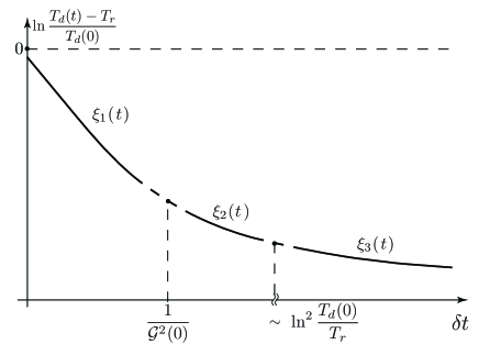
Figure 4: The dynamics of temperature relaxation, $g\ll 1$, $T_{d}(0)\gg T_{r}\exp\big{(}\pi^{2}/{\cal G}(0)\big{)}$. Here, $\xi_{1}(t)\sim-{\cal G}(0)\delta t,\ \ \xi_{2}(t)\sim-\sqrt{\delta t},\ \ \xi_{3}(t)\sim-{\cal G}_{r}\delta t.$

VI.4.2 Coulomb valley, $\bar{\Delta}\gg T_{d}(0)$

Now we consider the relaxation of the electron temperature on the island in the regime of Coulomb valley, $\bar{\Delta}\gg T_{d}(0)$. By using Eq. (84), we rewrite the quantum kinetic equation (25) as

$$\partial_{\tau}F_{\varepsilon}^{d}=\frac{\bar{g}\delta}{4\pi}\Biggl{(}F_{\varepsilon+\bar{\Delta}}^{r}-F^{d}_{\varepsilon}+\frac{1-F_{\varepsilon}^{d}F_{\varepsilon+\bar{\Delta}}^{r}}{B_{-\bar{\Delta}}}\Biggr{)}.$$ (102)

We remind that we consider the quasi-equilibrium regime. Then we need to add to the r.h.s. of Eq. (102) the collision integral $I^{(ee)}_{\varepsilon}$ which describes scattering due to electron-electron interaction in the island. In what follows we assume that the condition $T_{d}(0)\gg T_{r}$ holds. With the help of the following results

$$\int d\varepsilon\,\varepsilon(1-F^{d}_{\varepsilon}F^{r}_{\varepsilon-\omega})=T_{d}^{2}\operatorname{sgn}\omega\bigg{[}\frac{\omega^{2}}{T_{d}^{2}}-\frac{\pi^{2}}{3}\hskip 56.9055pt{}$$

$$-4{\rm li}_{2}(-e^{-|\omega|/T_{d}})+\frac{4|\omega|}{T_{d}}\ln\Big{(}1+e^{-|\omega|/T_{d}}\Big{)}\bigg{]},$$ (103)

$$B_{\omega}=\frac{2T_{d}}{\omega}\ln\left(2\cosh\frac{\omega}{2T_{d}}\right)$$ (104)

which are valid for $T_{r}\ll T_{d}$ (${\rm li}_{2}(z)=\sum_{n=1}^{\infty}z^{n}/n^{2}$ denotes the polylogarithmic function), we obtain from Eq. (102)

$$\frac{dT_{d}}{d\tau}=-\frac{3\delta\mathcal{G}(\tau)}{4\pi^{3}}T_{d}(\tau),$$ (105)

$$\ \mathcal{G}(\tau)=\frac{\bar{g}\bar{\Delta}}{T_{d}(\tau)}\exp\left(-\frac{\bar{\Delta}}{T_{d}(\tau)}\right).$$ (106)

We can estimate parameter $\lambda$ with logarithmic accuracy and find $\lambda=\ln E_{c}/\bar{\Delta}$ since the temperature of electrons in the island $T_{d}\ll\bar{\Delta}$. Therefore, both $\bar{g}$ and $\bar{\Delta}$ are independent of $\tau$. Integration of Eq. (102) yields

$$\frac{3\delta\bar{g}\tau}{4\pi^{3}}=h\left(\frac{\bar{\Delta}}{T_{d}(0)}\right)-h\left(\frac{\bar{\Delta}}{T_{d}(\tau)}\right)$$ (107)

$$h(z)=e^{z}/z-{\rm Ei}(z).$$ (108)

Here ${\rm Ei}(z)=-\int_{-z}^{\infty}dt\exp(-t)/t$ stands for the integral exponential. By using the asymptotic $h(z)=\exp(z)/z^{2}$ at $z\gg 1$, we obtain

$$\mathcal{G}(\tau)=\mathcal{G}(0)\Biggl{[}1+\frac{T_{d}(0)}{\bar{\Delta}}\ln\Big{(}1+\frac{3\delta\bar{\Delta}\mathcal{G}(0)\tau}{4\pi^{3}T_{d}(0)}\Big{)}\Biggr{]}^{-1}$$

$$\times\Biggl{[}1+\frac{3\delta\bar{\Delta}\mathcal{G}(0)\tau}{4\pi^{3}T_{d}(0)}\Biggr{]}^{-1}$$ (109)

and

$$T_{d}(\tau)=T_{d}(0)\Biggl{[}1+\frac{T_{d}(0)}{\bar{\Delta}}\ln\Big{(}1+\frac{3\delta\bar{\Delta}\mathcal{G}(0)\tau}{4\pi^{3}T_{d}(0)}\Big{)}\Biggr{]}^{-1}.$$ (110)

The results (109) and (110) are valid at not too long times

$$\tau\ll\frac{4\pi^{3}T_{d}(0)}{3\delta\bar{\Delta}\mathcal{G}(0)}\exp\left(\frac{\bar{\Delta}}{T_{r}}\right).$$ (111)

As expected, due to the exponentially small SET conductance in the sequential tunneling regime, the temperature relaxation is very slow, namely, logarithmical. Therefore, it is instructive to consider contribution to the temperature relaxation due to the electron co-tunneling.

VI.4.3 Inelastic cotunneling regime

As known very well, due to exponential suppression of the sequential tunneling mechanism deep in the Coulomb valley, $T_{d}\ll\bar{\Delta}$, the higher order process of inelastic cotunneling dominates the transport. nazarov Contrary to the case of sequential tunneling, the cotunneling contribution to the collision integral in the r.h.s. of Eq. (25) comes from frequencies of order $\omega\sim T_{d}\ll\bar{\Delta}$.

In the pseudo-fermion technique the inelastic cotunneling is revealed as the broadening of delta-peaks in the imaginary part of the retarded and advanced pseudo-fermion Green functions. schoeller ; burmistrov2 After taking into account Eq. (83), the integrand in Eq. (73) becomes of a complex pole structure. There are two pairs of proximal poles

$$\begin{split}\varepsilon&=\xi_{+}\pm i\bar{g}\Gamma_{+}(\bar{\xi}_{+}),\\ \varepsilon&=\xi_{-}-\omega\pm i\bar{g}\Gamma_{-}(\bar{\xi}_{-}).\end{split}$$ (112)

There is an additional series of Matsubara-type poles resulting from distribution functions $\mathcal{F}_{\epsilon}^{+}$ and $\mathcal{F}_{\epsilon+\omega}^{-}$. They lead to logarithmically divergent sums. The latter are controlled by the renormalization scheme. In our case all leading logarithms are absent. They have already been absorbed into renormalized constants $\bar{g}$ and $\bar{\Delta}$ by the proper choice of reference energy scale. Thus we can omit all divergent sums over Matsubara frequencies. Expanding in the $\omega/\bar{\Delta}$ we obtain

$$\,\textrm{Im}\,{\cal D}^{R}_{\omega,\rm pf}=\frac{\bar{g}Z^{2}\omega}{8\pi}\frac{{\cal F}^{+}+{\cal F}^{-}}{\bar{\Delta}^{2}},\ \ |\omega|\ll|\bar{\Delta}|.$$ (113)

Next we use the same arguments that led us to leading order espression (75). The function $\,\textrm{Im}\,{\cal D}^{R}_{\omega}$ then reads

$$\,\textrm{Im}\,{\cal D}^{R}_{\omega}=-\frac{\bar{g}Z^{2}}{4\pi}\frac{\omega}{\bar{\Delta}^{2}},\ \ |\omega|\ll|\bar{\Delta}|.$$ (114)

Using Eq. (114), we rewrite the quantum kinetic equation (25) as

$$\partial_{\tau}F_{\varepsilon}^{d}=\frac{\bar{g}^{2}\delta}{16\pi^{3}\bar{\Delta}^{2}}\int d\omega\,\omega\Biggl{[}\left(F_{\varepsilon-\omega}^{r}-F^{d}_{\varepsilon}\right)B_{\omega}+1-F_{\varepsilon}^{d}F_{\varepsilon-\omega}^{r}\Biggr{]}.$$ (115)

We remind that we consider the quasi-equilibrium regime. We mention that Eq. (115) coincides with the kinetic equation derived for the cotunneling regime in Ref. [BaskoKravtsov, ]. Then we need to add to the r.h.s. of Eq. (115) the collision integral $I^{(ee)}_{\varepsilon}$ which describes scattering due to electron-electron interaction in the island.

In the case of $T_{d}-T_{r}\ll T_{r}$, we obtain

$$\frac{dT_{d}}{d\tau}=-\frac{3\delta\mathcal{G}_{r}}{5\pi}(T_{d}-T_{r})$$ (116)

where $\mathcal{G}_{r}=\bar{g}^{2}T_{r}^{2}/(6\bar{\Delta}^{2})$ stands for the equilibirum SET conductance in the cotunneling approximation. In the opposite case $T_{d}\gg T_{r}$, by using Eq. (115), we find the following equations:

$$\frac{dT_{d}}{d\tau}=-\frac{3\delta\mathcal{G}(\tau)}{20\pi}T_{d}(\tau),$$ (117)

$$\mathcal{G}(\tau)=\frac{\bar{g}^{2}T_{d}^{2}(\tau)}{6\bar{\Delta}^{2}}$$ (118)

which govern the temperature relaxation. It is worthwhile to mention that if one substitutes $\mathcal{G}_{r}$ by $\mathcal{G}(\tau)$ in Eq. (116) then it becomes similar to Eq.(4) of Ref. [beloborodov4, ] for $V=0$ and in the absence of phonons. However, due to different numerical coefficients in the right hand side of Eqs. (116) and (117) such substitution is impossible even on the level of interpolating expression. Therefore, in the case $T_{d}-T_{r}\sim T_{r}$ one needs to solve Eq. (115) numerically.

Though, Eq. (116) leads to the standard exponential relaxation, Eq. (117) results in the relaxation according to the power-law. Indeed, solving Eqs. (117)-(118), we obtain

$$\mathcal{G}(\tau)=\mathcal{G}(0)\left(1+\frac{3\delta\mathcal{G}(0)\tau}{10\pi}\right)^{-1}$$ (119)

and

$$T_{d}(\tau)=T_{d}(0)\left[1+\frac{3\delta\mathcal{G}(0)\tau}{10\pi}\right]^{-1/2}$$ (120)

Eqs. (119) and (120) are valid at times

$$\tau\ll\frac{10\pi}{3\delta\mathcal{G}(0)}\frac{T_{d}^{2}(0)}{T_{r}^{2}}.$$ (121)

VII Discussions and conclusions

We have studied the relaxation dynamics of the SET under essentially non-equilibrium conditions. The language of kinetic equations happened to be the most adequate for this task. Analytical results are procured in the limiting cases of weak $g\gg 1$ and strong $g\ll 1$ Coulomb blockade. All relaxation equations (see Eqs. (48),(85),(96),(105)) obtained in the course reveal a pleasant generality. Namely,

$$\dot{X}_{d}\sim-\delta\mathcal{G}(X_{d})(X_{d}-X_{r}).$$ (122)

Here $X_{d}$ is a relaxing physical quantity (temperature, distribution function), and $\mathcal{G}(X_{d})$ is conductance of a SET which depends on $X_{d}$. Equation (122) has a transparent intuitive interpretation. Namely, the characteristic time scale determined by the r.h.s. of Eq. (122) is simply a dwell time of a particle inside the metallic island, Bagrets i.e. $\tau_{E}^{-1}\sim\mathcal{G}\delta$. The inverse dwell time can be also estimated as the ratio of the thermal conductance $\kappa$ to the heat capacitance of the island. The latter is proportional to $T_{d}/\delta$. The generality of Eq. (122) is, however, deceptive as it leads to drastically different evolution of physical quantities over time in the case of small and large values of $g$.

In the course of all our analysis we generally discarded the influence of electron-phonon (e-ph) interaction. The reasoning behind this is as follows. The e-ph scattering rate was well studied for 2-dimensional electron gas with disorder. mittal The following estimate has been found

$$\tau^{-1}_{\rm e-ph}\approx 8.3\times 10^{8}\,T^{3}\ [s^{-1}K^{-3}].$$ (123)

The electron-electron (e-e) scattering rate in mesoscopic systems is widely studied as well (see, e.g.[Blanter, ]). For small diffusive electron systems and for $T\ll E_{\rm Th}$ there are two parametrically different situations SivanImryAronov ; Blanter

$$\tau^{-1}_{\rm ee}\sim\frac{T^{2}\delta}{E_{\rm Th}^{2}},\ \ L\gg\mathcal{L}_{\mathbb{D}},\ \$$ (124)

$$\tau^{-1}_{\rm ee}\sim\frac{T^{2}}{E_{F}},\ \ L\ll\mathcal{L}_{\mathbb{D}},$$ (125)

where ${\cal L}_{\mathbb{D}}=(k_{F}l)^{\frac{2}{4-\mathbb{D}}}/k_{F}$ and $L$ stands for the size of the island. Equation (125) is a typical Fermi-liquid expression coming from large momenta of the order of the inverse screening length.The upper one comes from momenta $k\sim 1/L$ and of diffusive origin. Let us address the question which kind of dissipation dominates in various parametric regimes. The relaxation due to electron tunneling can be roughly estimated as

$$1/\tau_{E}\sim{\cal G}\delta.$$ (126)

By comparing Eqs. (124), (125) and (126), one can see that both quasi-equilibrium and non-equilibrium regimes can occur for $g\gg 1$ and $g\ll 1$. The non-equilibrium regime prevails for $g\gg 1$ while the quasi-equilibrium one dominates for $g\ll 1$ (see Figs. 5 and 6).

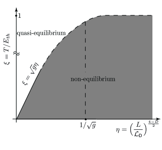
Figure 5: Schematic diagram of different regimes for $g\gg 1$. The non(quasi)-equilibrium regime dominates in (un)shaded region.

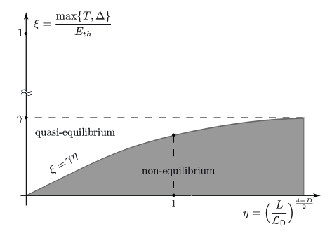
Figure 6: Schematic diagram of different regimes for $g\ll 1$. The non(quasi)-equilibrium regime dominates in (un)shaded region. At $\Delta=0$, $\gamma=\sqrt{g}$ and $\gamma=g$ in the cotunneling case for $T\ll\Delta$.

To estimate e-e scattering rate we use some experimental data taken from the experiment by Pasquer et al. glattli where they studied the Coulomb blockade effects in a small island of two-dimensional electron gas. The experimental data were as follows: the level spacing $\delta\approx 85\ mK$, the Fermi energy $E_{F}\approx 47\ K$, the elastic mean free path $l\approx 15\ \mu m$, the size of an island $L\approx 1\ \mu m$. This allows us to estimate the Thouless energy $E_{\rm Th}\approx 8\ K$ and e-e relaxation rate

$$\tau_{\rm ee}^{-1}\approx 1.7\times 10^{8}\,T^{2}\ [K^{-2}s^{-1}].$$ (127)

The typical temperature of the contemporary mesoscopic experiment is $T\lesssim 100\ mK$. As we see, with lowering temperature the e-ph scattering rate decays faster then the corresponding electron-electron (e-e) rate. On the other hand for the same metallic island the typical relaxation rate due to electron escape to reservoirs is

$$\tau_{E}^{-1}\sim g\times 10^{8}\ [s^{-1}]$$ (128)

Estimates (123)-(128) show that for all relevant experimental temperatures the phonons are frozen and e-ph interaction can safely be discarded. Next, comparing estimates (127) and (128) we conclude that varying $g$ two different parametric regimes explored in this paper can indeed be realized in the experiment. Namely, fully non-equilibrium regime is realized when $g$ is large enough and electron distribution function is arbitrary inside the island. The quasi-equilibrium regime persists in the opposite limit, when $g$ is small enough.

In addition to the relaxation of the electron distribution in the island due to escape of electrons to the reservoirs which we consider in details above there is another mechanism of energy relaxation which is due to interaction $U_{ir}$ of electrons in the island with electrons in the reservoirs. For a sake of simplicity we assume that the typical interaction parameter $r_{s}\sim 1/(k_{F}a_{B})\sim 1$ with $a_{B}$ standing for Bohr radius. In the case $L\ll\mathcal{L}_{\mathbb{D}}$, the energy relaxation rate due to interaction $U_{ir}$ of electrons in the island with electrons in the reservoirs can be estimated as

$$\frac{1}{\tau_{ee}^{(ir)}}\sim[\nu_{d}U_{ir}(k_{F})]^{2}\frac{T^{2}}{E_{F}}.$$ (129)

Here $U_{ir}(k)$ denotes the Fourier transform of the interaction $U_{ir}(\bm{r})$. Provided the condition $k_{F}d\gg 1$ holds $U_{ir}(k_{F})$ is strongly suppressed, $\nu_{d}U_{ir}(k_{F})\ll 1$, and

$$\frac{1}{\tau_{ee}^{(ir)}}\ll\frac{1}{\tau_{ee}}.$$ (130)

In the opposite case of large island, $L\gg\mathcal{L}_{\mathbb{D}}$, and for $a_{B}\ll L$ the estimate for the energy relaxation rate $1/\tau_{ee}^{(ir)}$ becomes

$$\frac{1}{\tau_{ee}^{(ir)}}\sim\frac{U^{2}_{ir}(k_{L})}{U^{2}(k_{L})-U^{2}_{ir}(k_{L})}\frac{1}{\nu_{d}U(k_{L})}\frac{T^{2}}{E_{Th}^{2}}\delta.$$ (131)

Here $k_{L}\sim 1/L$ and $U(k)$ stands for the Fourier transform of interaction between electrons in the island $k=0$ component of which leads to the charging term $H_{c}$ in the hamiltonian (1). As one can see, both cases of $\tau_{ee}\gg\tau_{ee}^{(ir)}$ and $\tau_{ee}\ll\tau_{ee}^{(ir)}$ are possible for $L\gg\mathcal{L}_{\mathbb{D}}$.

For $d\ll L$ where $d$ stands for the typical size of the tunneling junction between the island and reservoir Eq. (131) can be simplified as

$$\frac{1}{\tau_{ee}^{(ir)}}\sim\frac{a_{B}}{d}\frac{T^{2}}{E_{Th}^{2}}\delta.$$ (132)

For the experiments by Pasquer et al. glattli we estimate the Bohr radius $a_{B}\approx 10\,nm$ and assume typical $d$ to be of the order of $100\,nm$. Therefore, we expect that the regime in which the main mechanism of the energy relaxation of electrons in the island is due to its escape to the reservoirs can be realized in a laboratory.

To summarize, we have explored heat transport and relaxation processes in a SET with large number of tunneling channels over a wide range of parameters. In the regime of linear response we obtained analytical expressions for transport coefficients (conductance, thermal conductance and the response of electric current to temperature difference) in the entire span of values of $g$. It is possible to shape the general relations for linear response coefficients into Fermi-liquid type form. There is however an important difference, namely: the tunneling density of states undergoes dramatic renormalization due to Coulomb interaction. The latter leads to violation of Wiedemann-Franz law: in the $g\gg 1$ limit the Lorentz ratio $\mathcal{L}$ acquires weak periodic dependence on gate voltage (the precursor of Coulomb blockade). The method of quantum kinetic equation supplemented with non-equilibrium AES action has allowed us to treat Coulomb interaction exactly. We have obtained the time evolution of electron temperature (in the quasi-equilibrium regime) and the distribution function (in the non-equilibrium regime) of a SET island due to particle escape to reservoir. The corresponding collision integral is always non-local in energy due to inelastic nature of tunneling processes: the radiation of plasmon $\varphi$ always accompanies the tunneling event. In general, this leads to highly complicated integro-differential kinetic equations. Surprisingly we have shown that kinetic equations can be reduced to simple differential ones in a number of wide parametric regimes, namely: $g\gg 1$ (weakly blockaded SET) and $g\ll 1$ (strongly blockaded SET in sequential tunneling approximation with renormalization taken into account). This simplification is achieved due to the presence of strong scale separation in the problem $g\delta\ll T_{d}$ or $g\delta\ll\varepsilon_{d}$. Indeed, the characteristic frequency at which the distribution function in the kinetic equation changes is $\omega\sim g\delta$, while the scale at which the renormalization due to the presence of Coulomb interaction occurs is $\omega\gtrsim T_{d}$ or $\omega\gtrsim\varepsilon_{d}$. This separation is that allows us at first to treat Coulomb interaction and secondly to study evolution of the distribution function.

Still, quantum fluctuations of charge significantly change the relaxation laws comparing to simple exponential ones which are characteristic of semi-classical physics for $g\gg 1$ and of orthodox theory for $g\ll 1$. The regime  $g\ll 1,\ \Delta\gg T$ is dominated by cotunneling process. In the latter case the kinetic equation retains its integro-differential structure and is to be solved numerically elsewhere. Measurements of the predicted relaxation dynamics are an experimental challenge.

Appendix A Keldysh form of AES action

For a benefit of a general reader, we outline here the details of the derivation of the Keldysh form of AES-action from hamiltonian (1)-(4). To get rid of unsuitable quartic electron-electron interaction term (4) we decouple it via Hubbard-Stratonovich bosonic field $\varphi(t)$. After that the initial electron operators are gauge-transformed according to

$$d^{\dagger}_{\alpha}(t)\rightarrow d^{\dagger}_{\alpha}(t)e^{i\varphi(t)},\qquad d_{\alpha}(t)\rightarrow d_{\alpha}(t)e^{-i\varphi(t)},$$ (133)

the action of the system becomes gaussian in fermions:

$$\begin{split}S&=S_{0}+S_{c}+S_{t},\\ S_{0}&=\int_{\gamma}\sum_{\alpha}d_{\alpha}^{\dagger}(i\partial_{t}-\varepsilon_{\alpha}^{(d)})d_{\alpha}\\ &+\int_{\gamma}\sum_{k}a_{k}^{\dagger}(i\varepsilon_{t}-\varepsilon_{k}^{(r)})a_{k},\\ S_{c}&=\frac{1}{4E_{c}}\int_{\gamma}\dot{\varphi}^{2}dt+q\int_{\gamma}\dot{\varphi}dt,\\ S_{t}&=-\int_{\gamma}\sum_{k,\alpha}\Big{(}t_{k\alpha}a_{k}^{\dagger}d_{\alpha}e^{i\varphi}+\hbox{H.c.}\Big{)}dt.\end{split}$$ (134)

Here, for a sake of simplicity, we consider an island connected to a single reservoir. Superscript $d$ refers to the island and $r$ - to the reservoir. The integrals are understood as contour ones and $\gamma$ is the Keldysh contour. Integrating out fermions we obtain the effective action for the bosonic field $\varphi$:

$$S_{\rm eff}=-i{\rm tr}\,\ln(\widehat{G}^{-1}+\widehat{T})+S_{c}.$$ (135)

Here, matrices $\widehat{G},\ \widehat{T}$ have the following structure in the reservoir-island space:

$$\begin{split}&\widehat{G}=\begin{pmatrix}G_{k,d}\ &\ 0\\ 0\ &\ G_{\alpha,r}\end{pmatrix},\ \ \widehat{T}=\begin{pmatrix}0\ &\ t_{k\alpha}X\\ t^{\dagger}_{\alpha k}X^{\dagger}\ &\ 0\end{pmatrix},\\ &X=\frac{1}{\sqrt{2}}\begin{pmatrix}X_{c}\ &\ X_{q}\\ X_{q}\ &\ X_{c}\end{pmatrix},\end{split}$$ (136)

where $X_{c,q}$ are defined in Eq.(15). Expanding $S_{\rm eff}$ to the second order in $\widehat{T}$, we find

$$S_{\rm eff}=\frac{i}{2}{\rm tr}\,\Big{[}\widehat{G}\widehat{T}\widehat{G}\widehat{T}\Big{]}+S_{c}.$$ (137)

This expansion is valid in the limit $g_{ch}\ll 1$ and $N_{\rm ch}\gg 1$. Computing all the traces we recover the dissipative part of AES-action in form (16) with the polarization operator $\Pi$ given by the following general expressions:

$$\begin{split}\Pi^{R,A}(t,t^{\prime})&=\frac{i}{2g}\sum_{k,\alpha}|t_{k\alpha}|^{2}\Big{(}G_{k,r}^{K}(t^{\prime},t)G_{\alpha,d}^{R,A}(t,t^{\prime})\\ &+G_{k,r}^{A,R}(t^{\prime},t)G_{\alpha,d}^{K}(t,t^{\prime})\Big{)},\\ \Pi^{K}(t,t^{\prime})&=\frac{i}{2g}\sum_{k,\alpha}|t_{k\alpha}|^{2}\Big{(}G_{k,r}^{K}(t^{\prime},t)G_{\alpha,d}^{K}(t,t^{\prime})\\ &+G_{k,r}^{R}(t^{\prime},t)G_{\alpha,d}^{A}(t,t^{\prime})+G_{k,r}^{A}(t^{\prime},t)G_{\alpha,d}^{R}(t,t^{\prime})\Big{)}.\end{split}$$ (138)

Provided the density of states of electrons on the island and in the reservoir are slow varying near the Fermi energy, we can perform the summation over $\alpha$ and $k$ with the help of Eqs. (6)-(8) and reproduce the kernel of the action in form of Eq. (17).

Appendix B Electron’s self-energy

Here, we present the expressions for electron’s self-energy to substantiate the derivation of the kinetic equation in Sec. III. As follows from Fig. 2 a the lowest order (in $1/N_{\rm ch}$) contribution to the electron’s self-energy is given by

$$\begin{split}&\Sigma^{R,A}(t,t^{\prime})=i\sum\limits_{\alpha\alpha^{\prime}}(2\pi)^{2}[\delta(\epsilon_{\alpha})\delta(\epsilon_{\alpha^{\prime}})]^{1/2}\\ &\times\sum\limits_{k}t^{\dagger}_{\alpha k}t_{k\alpha^{\prime}}\Bigl{[}{G}^{R,A}_{k,r}(t,t^{\prime}){\cal D}^{K}(t,t^{\prime})+{G}^{K}_{k,r}(t,t^{\prime}){\cal D}^{R,A}(t,t^{\prime})\Bigr{]}\\ &\Sigma^{K}(t,t^{\prime})=i\sum\limits_{\alpha\alpha^{\prime}}(2\pi)^{2}[\delta(\epsilon_{\alpha})\delta(\epsilon_{\alpha^{\prime}})]^{1/2}\\ &\times\sum\limits_{k}t^{\dagger}_{\alpha k}t_{k\alpha^{\prime}}\Bigl{[}{G}^{K}_{k,r}(t,t^{\prime}){\cal D}^{K}(t,t^{\prime})+[{G}^{R}_{k,r}(t,t^{\prime})-{G}^{A}_{k,r}(t,t^{\prime})]\\ &\times[{\cal D}^{R}(t,t^{\prime})-{\cal D}^{A}(t,t^{\prime})]\Bigr{]}\end{split}$$ (139)

In case of constant densities of states in the island and the reservoir, they can be simplified with the help of Eqs. (6)-(8) and, then, written in the form of Eq. (22).

Appendix C Tunneling density of states on the island

The tunneling density of states of electrons inside the island is defined via corresponding full retarded Green’s function of original fermionic operators:

$$\begin{split}i{\bf G}^{R}_{d}(t,t^{\prime})&=\frac{1}{2}\big{\langle}d_{+}\bar{d}_{+}^{\prime}e^{-i(\varphi_{+}-\varphi_{+}^{\prime})}-d_{+}\bar{d}_{-}^{\prime}e^{-i(\varphi_{+}-\varphi_{-}^{\prime})}\\ &+d_{-}\bar{d}_{+}^{\prime}e^{-i(\varphi_{-}-\varphi_{+}^{\prime})}-d_{-}\bar{d}_{-}^{\prime}e^{-i(\varphi_{-}-\varphi_{-}^{\prime})}\big{\rangle}\\ &=-\frac{1}{2}\big{\{}G^{R}_{t,t^{\prime}}D^{K}_{t^{\prime},t}+G^{K}_{t,t^{\prime}}D^{A}_{t^{\prime},t}\big{\}}\end{split}$$ (140)

Here, operators $d_{\pm}\equiv d_{\pm}(t),\ d^{\prime}_{\pm}\equiv d_{\pm}(t^{\prime})$ are the gauge transformed operators of electrons inside the island (see Eq. 133.) Subscripts $\pm$ correspond to upper(lower) branch of Keldysh contour.

Switching to Wigner transform we obtain

$${\bf G}^{R}_{d}(\varepsilon)={-}\sum_{\alpha}\int\Big{\{}G^{R}_{\alpha,d}(\varepsilon+\omega)\mathcal{B}_{\omega}\,\textrm{Im}\,\mathcal{D}^{R}_{\omega}$$

$$+\mathcal{D}^{A}_{\omega}F^{d}_{\varepsilon+\omega}\,\textrm{Im}\,G^{R}_{d}(\varepsilon+\omega)\Big{\}}\frac{d\omega}{2\pi}.$$ (141)

Then, the tunneling density of states of electrons on the island becomes

$$\nu_{d}(\varepsilon)=-\frac{1}{\pi}\,\textrm{Im}\,{\bf G}^{R}_{d}(\varepsilon)=\nu_{d}\int\,\textrm{Im}\,\mathcal{D}^{R}_{\omega}\Big{\{}\mathcal{B}_{\omega}-F^{d}_{\varepsilon+\omega}\Big{\}}\frac{d\omega}{2\pi}.$$ (142)

Eq. (142) gives the tunneling density of states of electrons on the island in a non-equilibrium regime with arbitrary electron distribution function $F_{d}$. In the equilibrium, it leads to the result (33).

Appendix D Renormalization of AES-action at $g\gg 1$.

In this appendix we present details of derivation of Eq. (41) which describes renormalization of $g$ under non-equilibrium conditions in the weak-coupling regime. According to general philosophy behind renormalization we successively integrate partition-function over high-energy components of field $\varphi$. We split the scalar field into slow and fast components $\varphi\rightarrow\varphi+\theta$, where $\varphi=(\varphi_{c},\varphi_{q})$ and $\theta=(\theta_{c},\theta_{q})$, and expand the action up to quadratic order in the fast field $\theta$:

$$\begin{split}&S[\varphi]\rightarrow S[\varphi]+\int b_{t}[\varphi]\theta(t)\,dt+\frac{1}{2}\int\theta(t)K^{-1}_{t,t^{\prime}}[\varphi]\theta(t^{\prime})\,dtdt^{\prime},\\ &b_{t}[\varphi]=\frac{\delta S}{\delta\varphi(t)}\Big{|}_{\theta=0},\quad K_{t,t^{\prime}}^{-1}[\varphi]=\frac{\delta^{2}S}{\delta\varphi(t)\delta\varphi(t^{\prime})}\Big{|}_{\theta=0}.\end{split}$$ (143)

Next we integrate out the fast components $\theta$ and obtain the effective action for the slow components:

$$S_{\rm eff}[\varphi]=S[\varphi]-\frac{1}{2}\int\frac{d\omega_{1}d\omega_{2}}{(2\pi)^{2}}b_{\omega_{1}}^{\dagger}K_{\omega_{1}\omega_{2}}b_{\omega_{2}}+\frac{i}{2}\operatorname{tr}\ln K$$

$$=S[\varphi]-S_{I}+S_{II}.$$ (144)

Here, frequencies $\omega_{1},\omega_{2}$ lie in the energy window $[\underline{\Lambda},\overline{\Lambda}],\ \underline{\Lambda}<\overline{\Lambda}$. The trace is understood to be over the frequencies in the same window as well as in the Keldysh space. High energy scale $\overline{\Lambda}$ in the AES-action is naturally set by the first term in Eq. (14): $\overline{\Lambda}\sim gE_{c}$. Note that the linear in $\theta(t)$ term in (143) does not generally disappear. But, as will be proven below, it is irrelevant since it leads to $1/\overline{\Lambda}$ corrections.

Next we perform the following decomposition

$$K^{-1}[\varphi]=K^{-1}[0]+\Big{(}K^{-1}[\varphi]-K^{-1}[0]\Big{)}$$

$$\equiv K^{-1}[0]+\delta K^{-1}[\varphi]$$ (145)

and treat the last term perturbatively. The operator $K^{-1}[0]$ determines a fast field propagator. It corresponds to perturbative Green function of the AES-action and follows from Eqs. (16)-(17):

$$K^{R}(t,t^{\prime})=-i\langle\varphi_{c}(t)\varphi_{q}(t^{\prime})\rangle,\,K^{A}(t,t^{\prime})=-i\langle\varphi_{q}(t)\varphi_{c}(t^{\prime})\rangle,$$

$$K^{K}(t,t^{\prime})=-i\langle\varphi_{c}(t)\varphi_{c}(t^{\prime})\rangle.$$ (146)

In the leading order the Wigner transform of the perturbative Green functions are given as

$$\begin{split}K^{R}_{\omega}&=K^{A\dagger}_{\omega}=-\frac{4\pi i}{g}\left(\int(F^{d}_{\varepsilon}-\frac{1}{g}\sum\limits_{\alpha}g_{\alpha}F^{\alpha}_{\varepsilon-\omega})\,d\varepsilon\right)^{-1},\\ K^{K}_{\omega}&=2i\operatorname{Im}K^{R}_{\omega}B_{\omega},\end{split}$$ (147)

where we neglect all time derivatives with respect to slow time since we are interested in high frequencies. The physical electron distribution function is bound to have sign-function as its limit at infinity $F_{\varepsilon}\rightarrow\operatorname{sgn}(\varepsilon),\ \varepsilon\rightarrow\infty$. This yields the result

$$\begin{split}K^{R}_{\omega}&=K^{A\dagger}_{p,\omega}=-\frac{2\pi i}{g}\frac{1}{\omega+\Delta Q\delta},\\ B_{\omega}&=\frac{\sum\limits_{\alpha}g_{\alpha}\int d\varepsilon(1-F^{d}_{\varepsilon}F^{\alpha}_{\varepsilon-\omega})}{2g(\omega+\Delta Q\delta)},\\ \Delta Q&=\frac{\nu_{d}}{2}\sum_{\alpha}\int d\varepsilon\Bigl{[}F_{\varepsilon}^{d}-\frac{g_{\alpha}}{g}F_{\varepsilon}^{\alpha}\Bigr{]}.\end{split}$$ (148)

In general, $\Delta Q$ does not vanish. Next we find

$$\begin{split}S_{I}&=\frac{1}{2}\int\frac{d\omega}{2\pi}\int dtdt^{\prime}b(t)^{\dagger}K[0]_{\omega}e^{-i\omega(t-t^{\prime})}b(t^{\prime})\\ &-\frac{1}{2}\int\frac{d\omega_{1}d\omega_{2}}{(2\pi)^{2}}\int dtdt^{\prime}b^{\dagger}(t)e^{-i\omega_{1}(t-t_{1})}K_{\omega_{1}}[0]\\ &\times\delta K^{-1}[\varphi]_{t_{1}t_{2}}K_{\omega_{2}}[0]e^{-i\omega_{2}(t_{2}-t^{\prime})}b(t^{\prime}).\end{split}$$ (149)

Performing integrations over fast frequencies $\omega,\ \omega_{1},\ \omega_{2}$ we see that the first integral is $\sim 1/((t-t^{\prime})\overline{\Lambda})$ and the second one is $\sim 1/((t-t_{1})(t^{\prime}-t_{2})\overline{\Lambda}^{2})$. Thus they are irrelevant for RG-analysis. It means that only term $S_{II}$ contains logarithmic in $\overline{\Lambda}$ corrections.

As usual we are interested in the first non-vanishing $\varphi$-dependent correction:

$$S_{II}\rightarrow\frac{i}{2}\operatorname{tr}\Big{\{}K[0]\delta K^{-1}[\varphi]\Big{\}}.$$ (150)

Working out the trace in Eq. (150) we obtain

$$\begin{split}S_{II}&=-\frac{i}{2}\int dtdt^{\prime}\Bigg{[}\int\limits_{\overline{\Lambda}>|\omega|>\underline{\Lambda}}K^{K}_{\omega}(\tau)\frac{d\omega}{2\pi}\Bigg{]}\\ &\times\Big{(}\bar{X}_{c}(t)\bar{X}_{q}(t)\Big{)}\begin{pmatrix}0&\Pi^{A}(t,t^{\prime})\\ \Pi^{R}(t,t^{\prime})&\ \Pi^{K}(t,t^{\prime})\end{pmatrix}\begin{pmatrix}X_{c}(t^{\prime})\\ X_{q}(t^{\prime})\end{pmatrix}.\end{split}$$ (151)

Substituting it into (144) we see, that the structure of the AES-action is restored. The only difference is the change of the coupling constant given by Eq. (41). Finally, we mention that in the case of non-zero $\Delta Q$ Eq. (45)should be changed to $\omega_{0}\sim\max\{\varepsilon_{d},T_{r},T_{l},|\Delta Q|\delta\}$.

Appendix E Renormalization of the pseudo-fermion action

Here we provide details of the renormalization of the pseudo-fermion action (63) which are used in Sec. VI.

E.1 Renormalization of $Z$, $\Delta$,  and $g$.

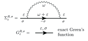
Figure 7: The Dyson equation for pseudo-fermion self-energy.

The exact pseudo-fermion Green’s function can be written as

$$\overline{G}^{R}_{\varepsilon,\sigma}=\frac{1}{\varepsilon-\xi_{\sigma}-\Sigma^{R,\sigma}_{\varepsilon}}.$$ (152)

Here, $\xi_{\sigma}=\Delta\sigma/2-\eta$. To write it in the renormalized form (79) we redefine the theory’s constants and write down the standard relations defining the Green’s function scaling $Z$, the renormalized gap $\bar{\Delta}$ and the Green’s function width $\Gamma^{\sigma}_{\varepsilon}$ respectively:

$$Z=\Big{(}1-\partial_{\varepsilon}\,\textrm{Re}\,\Sigma^{R,\sigma}\big{|}_{\varepsilon=\bar{\xi}_{\sigma}}\Big{)}^{-1},$$ (153)

$$\bar{\xi}_{\sigma}=\xi_{\sigma}+\,\textrm{Re}\,\Sigma^{R,\sigma}\big{|}_{\varepsilon=\bar{\xi}_{\sigma}},$$ (154)

$$i\bar{g}\Gamma^{\sigma}_{\varepsilon}=-iZ\,\textrm{Im}\,\Sigma^{R,\sigma}_{\varepsilon}.$$ (155)

To find the scaling $Z$ and relate $\bar{g}$, and $\bar{\Delta}$ to their bare counterparts we solve the one-loop Dyson equation for the self-energy presented in Fig. 7. With the help of (68) we find

$$\begin{split}\,\textrm{Re}\,\Sigma^{R,\sigma}_{\varepsilon}&=\frac{g}{4\pi}\int\frac{d\omega}{2\pi}\omega B_{\omega}Z(\omega)\\ &\times\,\textrm{Re}\,\frac{1}{\varepsilon+\omega\sigma-\bar{\xi}_{-\sigma}-iZ\,\textrm{Im}\,\Sigma^{-\sigma,R}_{\varepsilon+\omega\sigma}}\end{split}$$ (156)

It is important to understand that scaling parameter $Z$ cannot be put before the sign of an integral. Generally it is cut-off dependent and contains the factor $\ln(\Lambda/\omega_{0})$, where $\Lambda$ is an ultraviolet cut-off of the theory ($E_{c}$ in our case) while $\omega_{0}$ is a characteristic scale of the Green’s function entering the integrand. To determine $\omega_{0}$ we notice that the integral in (156) diverges, being determined by the behavior of the integrand in the large $\omega$ limit. That is why the characteristic scale of the Green’s function entering (156) is its running frequency: $\omega_{0}\sim\omega$. Solving Eqs. (156) and (153) with logarithmic accuracy we obtain

$$\frac{1}{Z^{2}(\Lambda)}\frac{\partial Z(\Lambda)}{\partial\Lambda}=\frac{g}{4\pi^{2}}\frac{B(\Lambda)Z(\Lambda)}{\Lambda}$$ (157)

Integrating (157) in the limits $[\omega_{0},E_{c}]$ we recover (80) in complete analogy with equilibrium case. Thus, the renormalization procedure is outlined and the rest of formulae (79)-(81) are obtained in a similar fashion.

E.2 Callan-Symanzik equation for $\langle\mathcal{N}\rangle_{pf}$.

The anomalous dimension $\gamma$ of $\langle\mathcal{N}\rangle$ is introduced as

$$Z^{\gamma}\overline{\langle\mathcal{N}\rangle}_{pf}(\bar{\Delta},\bar{g})=\langle\mathcal{N}\rangle_{pf}(\Delta,g,\Lambda).$$ (158)

To extract $\gamma$ we write down the corresponding Callan-Symanzik equation for: $\langle\mathcal{N}\rangle_{pf}(\Delta,g,\Lambda)=\sum_{\sigma}\langle\bar{\psi}_{\sigma}\psi_{\sigma}\rangle$. The tree-level $\langle\mathcal{N}\rangle_{pf}(\Delta,g,\Lambda)$ is given by Eq. (74). Following general strategy we write the corresponding Callan-Symanzik equation for the function $\langle\mathcal{N}\rangle_{pf}(\Delta,g,\Lambda)$ in the form:

$$\Big{(}\frac{\partial}{\partial\ln\Lambda}+\beta_{g}\frac{\partial}{\partial g}+\beta_{\Delta}\frac{\partial}{\partial\Delta}+\gamma\frac{g}{4\pi^{2}}\Big{)}\langle\mathcal{N}\rangle(g,\Delta,\Lambda)=0.$$ (159)

where the corresponding $\beta$ - functions are easily seen from Eq. (81):

$$\begin{split}\beta_{g}=\frac{g^{2}}{2\pi^{2}},\quad\beta_{\Delta}=\frac{g\Delta}{2\pi^{2}}.\end{split}$$ (160)

The term with $\beta_{g}$ always contains extra $g$ and can be dropped in the leading order.

To find $\gamma$ we need to find $\langle\mathcal{N}\rangle_{pf}$ in the next to the tree-level order. The diagram representing the correction to pseudo-fermion particle number is presented in Fig. 8. Calculating with logarithmic accuracy and using extensively the fact that ${\cal B}_{\omega}\rightarrow\operatorname{sgn}\omega$ at large $\omega$ we obtain

$$\begin{split}\langle\mathcal{N}\rangle_{pf}(\Delta,g,\Lambda)&=1-\frac{{\cal F}^{+}+{\cal F}^{-}}{2}\\ &-\frac{g}{8\pi^{2}}\Delta(\partial_{\eta}{\cal F}^{+}-\partial_{\eta}{\cal F}^{-})\int_{\omega_{0}}^{\Lambda}\frac{d\omega}{\omega}B(\omega).\end{split}$$ (161)

Plugging Eq. (161)) into Eq. (159)) we find that $\gamma=0$ that proves Eq. (82).

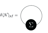
Figure 8: Correction to pseudo-fermion particle number $\langle\mathcal{N}\rangle_{pf}$.

References

- (1) G. Schön, A. Zaikin, Phys. Rep. 198, 237 (1990).
- (2) Z. Phys. B: Condens. Matter 85, 317 (1991), special issue on single charge tunneling, edited by H. Grabert and H. Horner.
- (3) Single Charge Tunneling, edited by H. Grabert and M.H. Devoret (Plenum, New York, 1992).
- (4) I. Aleiner, P. Brouwer, L. Glazman, Phys. Rep. 358, 309 (2002).
- (5) For a review, see L.I. Glazman and M. Pustilnik in New Directions in Mesoscopic Physics (Towards to Nanoscience, eds. R. Fazio, G. F. Gantmakher and Y. Imry (Kluwer, Dordrecht, 2003).
- (6) F. Giazotto, T.T. Heikkilä, A. Luukanen, A.M. Savin and J.O. Pekola, Rev. Mod. Phys. 78, 217 (2006).
- (7) R. Scheibner et al., New J. Phys. 10, 08306 (2008).
- (8) E.A. Hoffmann et al., NanoLett. 9, 779 (2009).
- (9) A.S. Dzurak et al., Phys. Rev. B 55, 10197 (1998).
- (10) R. Scheibner et al., Phys. Rev. B 75, 041301 (2007).
- (11) S. Möller, H. Buhmann, S.F. Godijn, and L.W. Molenkamp, Phys. Rev. Lett. 81, 5197 (1998).
- (12) M. Amman, E. Ben-Jacob, and J. Cohn, Z. Phys. B 85, 405 (1991).
- (13) C.W.J. Beenakker and A.A.M. Staring, Phys. Rev. B 46, 9667 (1992).
- (14) A.V. Andreev and K.A. Matveev, Phys. Rev. Lett. 86, 280 (2001).
- (15) M. Turek and K.A. Matveev, Phys. Rev. B 65, 115332 (2002).
- (16) K.A. Matveev and A.V. Andreev, Phys. Rev. B 66, 045301 (2002).
- (17) B. Kubala and J. König, Phys. Rev. B 73, 195316 (2006).
- (18) T. Nakanishi and T. Kato, Journal of the Physical Society of Japan 76, 034715 (2007).
- (19) X. Zianni, Phys. Rev. B 75 045344 (2007).
- (20) B. Kubala, J. König and J. Pekola, Phys. Rev. Lett. 100, 066801 (2008);
- (21) I.S. Beloborodov, A.V. Lopatin, F.W.J. Hekking, R. Fazio, V.M. Vinokur, Europhys. Lett. 69, 435 (2005).
- (22) V. Tripathi, Y.L. Loh, Phys. Rev. Lett. 96, 046805 (2006).
- (23) A. Glatz and I.S. Beloborodov, Phys. Rev. B 79, 041404(R) (2009).
- (24) A. Glatz and I.S. Beloborodov, Phys. Rev. B 79, 235403 (2009).
- (25) A. Glatz and I.S. Beloborodov, Europhys. Lett. 87, 57009 (2009).
- (26) D.M. Basko and V.E. Kravtsov, Phys. Rev. Lett. 93, 056804 (2004); Phys. Rev. B 71, 085311 (2005).
- (27) D. Bagrets and F. Pistolesi, Phys. Rev. B 75, 165315 (2007).
- (28) A. Altland and F. Egger, Phys. Rev. Lett. 102, 026805 (2009).
- (29) T. T. Heikkilä Yu. V. Nazarov, Phys. Rev. Lett. 102, 130605 (2009)
- (30) M. A. Laakso, T. T. Heikkilä and Yu. V. Nazarov arXiv:0912.2832
- (31) G.-L. Ingold and Yu.V. Nazarov, in Single Charge Tunneling, edited by H. Grabert and M. H. Devoret, NATO ASI, Ser. B, Vol. 294 (Plenum, New York, 1991).
- (32) N.M. Chtchelkatchev, V.M. Vinokur, T.I. Baturina, Phys. Rev. Lett. 103, 247003 (2009).
- (33) N.M. Chtchelkatchev, V.M. Vinokur, T.I. Baturina, arXiv:1003.6105
- (34) V. Ambegaokar, U. Eckern and G. Schön, Phys. Rev. Lett. 48, 1745 (1982).
- (35) I. S. Beloborodov, K. B. Efetov, A. Altland and F. W. J. Hekking Phys. Rev. B 63, 115109 (2001)
- (36) K.B. Efetov, A. Tschersich Phys. Rev. B 67, 174205 (2003).
- (37) A. Altland, L.I. Glazman, A. Kamenev, J.S. Meyer, Ann. Phys. 321, 2566 (2006).
- (38) A. Glatz and I.S. Beloborodov, Phys. Rev. B 81, 033408 (2010).
- (39) A. Glatz, I. S. Beloborodov, N. M. Chtchelkatchev, and V. M. Vinokur, arXiv:1005.5188.
- (40) R. Landauer, IBM J. Res. Dev. 1, 223 (1957).
- (41) M. A. Skvortsov, A. I. Larkin, M. V. Feigel’man, Phys. Rev. B 63, 134507 (2001).
- (42) J. Rammer, and H. Smith, Rev. Mod. Phys. 58, 323, (1986); A. Kamenev, A. Levchenko, Adv. in Phys. 58, 197 (2009).
- (43) B.L. Altshuler and A.G. Aronov, in Electron-Electron Interactions in Disordered Conductors, ed. A.J. Efros and M. Pollack, Elsevier Science Publishers, North-Holland, 1985.
- (44) A. Schmid, Z. Phys. 271, 251 (1974).
- (45) B.L. Altshuler and A.G. Aronov, JETP Lett. 30, 482 (1979).
- (46) I.O. Kulik and R.I. Shekhter, Zh. Eksp. Teor. Fiz. 68, 623 (1975) [Sov. Phys. JETP 41, 308 (1975)]; E. Ben-Jacob and Y.Gefen, Phys. Lett. A 108, 289 (1985); K.K. Likharev and A.B. Zorin, J. Low Temp. Phys. 59, 347 (1985); D.V. Averin and K.K. Likharev, J. Low Temp. Phys. 62, 345 (1986).
- (47) A. A. Abrikosov, Fundamentals of the theory of metals, North-Holland, Amsterdam (1988).
- (48) H. Schoeller and G. Schön, Phys. Rev. B 50, 18436 (1994).
- (49) A.A. Abrikosov, L.P. Gorkov, and I.E. Dzyaloshinski, Methods of Quantum Field Theory in Statistical Physics (Dover, New York, 1963).
- (50) I.S. Burmistrov and A.M.M. Pruisken, Phys. Rev. B 81, 085428 (2010).
- (51) S.E. Korshunov, Pis ma Zh. Eksp. Teor. Fiz. 45, 342 (1987) [JETP Lett. 45, 434 (1987)].
- (52) Formally, the integral in Eq. (48) for diverge at . Howerver, this divergence is due to the presence of unphysical zero mode of the boson field in the AES-action (13). Exclusion of this zero mode leads to substitution of for in Eqs. (48). Obviously, it does not affect the form of Eq. (49)
- (53) K.A. Matveev, Sov. Phys. JETP 72, 892 (1991).
- (54) A.A. Abrikosov, Physics 2, 21 (1965).
- (55) J. A. Rosch, P. Wölfle, Advances in Solid State Physics, vol. 42, p.175
- (56) N.S. Wingreen and Y. Meir, Phys. Rev. B 49, 11040 (1993).
- (57) A.I. Larkin and V.I. Melnikov, Zh. Eksp. Teor. Fiz. 61 1231 (1971) [Sov. Phys. JETP 34, 656 (1972)].
- (58) L. Zhu and Q. Si, Phys. Rev. B 66, 024426 (2002).
- (59) G. Zaránd and E. Demler, Phys. Rev. B 66, 024427 (2002).
- (60) D.V. Averin and Yu.V. Nazarov, Phys. Rev. Lett.65,2246 (1990)
- (61) A. Mittal Ph.D. thesis, Yale University (1996)
- (62) Ya.M. Blanter, Phys. Rev. B 54, 12807 (1996).
- (63) U. Sivan, Y. Imry, A.G. Aronov, Europhys. Lett. 28, 115 (1994).
- (64) C. Pasquer, U. Meirav, F. I. B. Williams, D. C. Glattli Y. Jin and B. Etienne Phys. Rev. Lett. 70, 69 (1993)