Roughness with a finite correlation length in the Microtrap

Abstract

We analyze the effects of roughness in the magnitude of the magnetic field produced by a current carrying microwire, which is caused by geometric fluctuation of the edge of wire. The relation between the fluctuation of the trapping potential and the height that atom trap lies above the wire is consistent with the experimental data very well, when the colored noise with a finite correlation length is considered. On this basis, we generate the random potential and get the density distribution of the BEC atoms by solving the Gross-Pitaevskii equation, which coincides well with the experimental image, especially in the number of fragmentations. The results help us further understand the nature of the fluctuation and predict the possible application in the precise measurement.

I INTRODUCTION

Trapping and manipulating ultracold atoms and Bose-Einstein condensations (BEC) in magnetic potential produced by micro atom chip attracted more attention recently because it is easy to perform coherent manipulation, transport and interferometry on a chip Folman ; Fort2007 , where the condensate is very close to the surface of wire. It is possible to bring miniaturization into the application of BEC Hansel . The trapping frequencies in the radial direction are normally several $kHz$, and a few $Hz$ in the axial direction. Hence the aspect ratio is so high that the size of BEC is several $mm$ in the axial direction, the spatial effects on the condensate will be obvious. However, for small-scale magnetic field of atom traps produced by micro fabricated current-carrying wires, an unexpected problem in these chips was their small fluctuation in magnetic field, which introduces a random potential along the trap. Such a fluctuation in potential will cause fragmentation of the atom clouds Fort2007 ; Leanhardt . The effects of the random potential have been studied theoretically Wang ; Schumm , where the randomness in magnetic field is due to geometric fluctuation of the wire surface and the strength of the disorder field shows a $d^{-5/2}$ relation with the height $d$ that atoms lie above the wire, when assuming the correlation of the wire edge is the white-noise correlation. It is not coincidental to the experimentally observed $d^{-2.2}$ relation Kraft .

The deviation in the theoretical calculations Wang ; Schumm from the experiment is caused by the white-noise approximation made, which does not meet the actual situation that the system’s fluctuation cannot be the ideal white noise palasantzas ; hinds . In this paper we elucidate the nature of the random potential, indicating the relation between the strength of the potential and the height of the BEC atoms. Different from the white-noise assumption, we consider a more general correlation form—the colored noise correlation $R(r)=\sigma^{2}e^{-|r|/\xi}$, with $\xi$ the correlation length of the system. Here we borrow the notion ’colored noise’ from the theory for time-domain noise analysis to deal with the case of spatial roughness Zhou . Our theory shows that the power index $\alpha$ in the disorder potential $u_{s}=C\cdot d^{-\alpha}$ is relevant to the system’s intrinsic correlation length $\xi$. This means by measuring the dependence factor $\alpha$, the correlation length of the current-carrying wire can be known. We point out in experiment  Kraft , $\alpha=2.2$ because $\xi=75\mu m$. Consequently, the correlation function for the random potential is calculated.

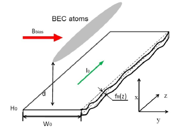
Figure 1: (Color online) A typical atomchip for BEC. A constant current $I_{0}$ flows in the z-direction of the wire with $H_{0}$ high and $W_{0}$ wide. The BEC atoms lie above the wire at the height of $d$. A bias magnetic field $B_{b}ias$ in the longitudinal direction produces a local minimum. $f_{R}(z)$ is the deviation of the edge from its ideal position.

With the random potential we solve the Gross-Pitaevskii equation, depict the density profile of the captured BEC atoms and compare it with that of the white-noise case. The desired random potential is generated using a selected aperture function derived from the correlation function. The number of fragmentations has a better agreement with the experiment than previous calculations. This work is meaningful in the simulation of transport process. It as well predicts a criterion for judging the quality of the wire used for cold-atom manipulation, which might be highly applicable in precise measurement.

II THE STRENGHTH OF THE DISORDER POTENTIAL

A typical setup of a magnetic microtrap is shown in Fig. 1. The current $I_{0}$ flowing in a micro-fabricated copper conductor in the z-direction and a bias field $B_{bias}$ in the y-direction form a magnetic trap for atoms. The distance $d$ from the surface of the current-carrying wire to the center of the trapping potential is controlled by the bias field and the current, $d=\mu_{0}I_{0}/2\pi B_{bias}$.

The random potential is brought about by the roughness in the magnetic trap for the BEC atoms lying above the wire surface about $100\mu m$ $\sim$ $200\mu m$. What we are interested is the z-direction of the random magnetic field $B_{z}$, which connects with the y-component of the current. In experiments Esteve ; Kraft , the wire normally is a thin electroplated gold layer of a few $\mu m$ thick. The surface of the wire can be made very flat technically with the electroplating method. So the main contribution of the random field arises from the side of the wire.

The distortion of the side edge of the wire curves the current flow. The potential roughness in the magnetic microtrap is induced by this abnormal current. To compute the fluctuation without loss of generality, we make the following assumptions. First the current $I_{0}$ remains constant on the edge of the wire, the amplitude $J_{0}$ of the current density $\vec{j}$ is then constant too. Second the resistivity keeps unchanged along the current-carrying wire. Third the deviation of the edge from its ideal position (both left and right) $f_{L/R}$ is trivial compared with the width of the wire $W_{0}$, $f_{L/R}/\ll W_{0}$. Considering symmetry, only $f(z)\equiv\frac{1}{2}(f_{L}(z)+f_{R}(z))$ contributes notably to the fluctuation, and $f^{-}=\frac{1}{2}(f_{L}-f_{R})$ is neglected.

If we ignore the change in the module of the current density vector, then we consider the effects due to the alteration of the direction of $\vec{j}$. The z-component of $\vec{B}$, i.e. $B_{z}$, is directly relevant to the y-component of current density. In yz plane the current density satisfies the charge conservation condition $\frac{\partial j_{y}}{\partial y}+\frac{\partial j_{z}}{\partial z}=0$. Under such assumptions, we introduce an auxiliary scalar potential $G$, so that $j_{y}=J_{0}\frac{\partial G}{\partial z}$ and $j_{z}=-J_{0}\frac{\partial G}{\partial y}$. The function $G$ satisfies the Laplace equation in the interior of the wire $\nabla^{2}G=0$. Using separation of variables, we get the Fourier component of $f(z)$ which brings a transverse current density Wang ,

$$j_{y}\propto J_{0}\frac{\partial}{\partial z}\int_{-\infty}^{\infty}\frac{e^{ikz}dk}{\sinh(kW_{0})}\cdot\cosh(ky)\sinh(kW_{0}/2)F_{f}$$ (1)

where $F_{f}$ is the inverse Fourier transform of $f(z)$, $F_{f}=\frac{1}{2}\int_{-\infty}^{\infty}dze^{ikz}f(z)$, and $k$ is the wave vector in the frequency domain.

Therefore the disorder magnetic field can be derived from the Bio-Savart law:

$$\vec{B}(\vec{r})=\frac{\mu_{0}}{4\pi}\int d^{3}\vec{r}\frac{\vec{j}\times\vec{r}}{r^{3}}$$ (2)

The random potential $U(z)$ is given by $U(z)=-\mu_{B}\cdot B_{z}$. So the strength of $U$ induced by the roughness in the magnetic microtrap can be measured by the value at the zero point of the potential’s auto-correlation function $g(r)$ with $r=z-z^{\prime}$,

$$g(r)=\langle\delta U(z)\delta U(z^{\prime})\rangle$$ (3)

$\langle\ldots\rangle$ denotes the ensemble average. And the Fourier transform of $g(r)$, i.e. the power spectral density of the random potential, is

$$S(k)=\int dre^{ikr}g(r)$$ (4)

As the wire is eletroplated with a thin layer of gold Esteve , it is acceptable to assume $H_{0}\ll d$ and ignore the thickness of the line. We substitute the dimensionless variable $\beta=kd$ for $k$ , and obtain

$$S(\beta)=Ad^{-4}\cdot\beta^{4}P(\beta)$$ (5)

with

$$P(\beta)=\frac{2\sinh(\beta W_{0}/2d)}{\sinh(\beta W_{0}/d)(\beta W_{0}/d)}\sum_{n=0}^{\infty}\frac{(-1)^{n}}{n!(2y)^{n}}K_{n+1}(y)\cdot$$

$$\gamma(2n+1,-\frac{\beta W_{0}}{2d},\frac{\beta W_{0}}{2d})\cdot F(\beta/d)$$ (6)

where $A$ is a constant, $F(k)=\int d(z-z^{\prime})e^{-ik(z-z^{\prime})}\langle f(z)f(z^{\prime})\rangle$, $K_{n}(x)$ the Bessel function of the second kind, and $\gamma(n,x_{1},x_{2})$ is the incomplete gamma function $\gamma(n,x_{1},x_{2})=\int_{x_{1}}^{x_{2}}dxx^{n-1}e^{-x}$. We then compute the inverse Fourier transform and get the disorder potential $u_{s}^{2}$.

$$g(z)=\mathcal{F}^{-1}[S(\beta)]=\frac{1}{d^{5}}\int_{-\infty}^{\infty}d\beta e^{ik(z-z^{\prime})}S(\beta)$$ (7)

$$u_{S}^{2}=g(0)\sim d^{-5}\int_{-\infty}^{\infty}dkF(k)$$ (8)

When the correlation of the wire edge fluctuation is white-noise form, $\langle f(z)f(z^{\prime})\rangle$ is a $\delta$ function, and $F(k)$ in Eq.(8) is a constant, we have $u_{s}^{2}\sim d^{-5/2}$, which is the same in Wang . The white noise condition when the edge of the wire totally not correlated is the simplified case, it limits the supremum of the system fluctuation. Below we discuss the colored-noise model with a finite correlation length.

III DEPENDENCE BETWEEN POTENTIAL AND HEIGHT FOR A FINITE CORRELATION LENGTH

The fluctuation $f(z)$ is described as a colored noise model. The function $f(z)$ is a Gaussian random variable with zero mean $\langle f(z)\rangle=0$, and variance palasantzas ; hinds

$$\langle f(z)f(z^{\prime})\rangle=\sigma^{2}e^{-|r|/\xi}$$ (9)

The colored noise given by Eq.(9) is parameterized by three key factors, the distance along the wire $r=z-z^{\prime}$, the characteristic correlation length $\xi$ and the noise strength $\sigma$. When $\xi\rightarrow 0$, it degenerates into the white-noise correlation form $\langle f(z)f(z^{\prime})=\delta(z-z^{\prime})$, which is the ideal situation of the roughness Wang ; Schumm . When $\xi\rightarrow\infty$, the surface of the wire becomes totally correlated, implying a perfect smooth surface, which is the ideal case of the wire. The power spectrum of Eq.(9) for the wire edge is

$$F(k)=\frac{2\xi}{1+\xi^{2}k^{2}}$$ (10)

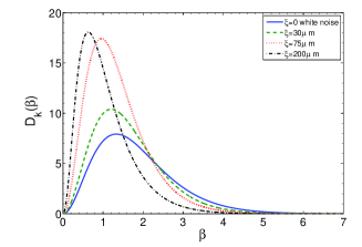
Figure 2: (Color online) The power spectral function of potential $S(\beta)$ for the different correlation length of disorder potential. The solid line is for white noise with $\xi=0\mu m$. Others are for the case of colored noise. The dashed line with $\xi=30\mu m$, the dotted line $\xi=75\mu m$, and the dash dotted line $\xi=200\mu m$.

When it comes to our model that the wire edge has an intrinsic randomness, the power spectral density of which described in Eq.(10) is moderate in comparison. The power spectral density of potential $S(\beta)$ for different correlation lengths is shown in Fig. 2. In the white-noise correlation $\xi=0\mu m$, the curve peaks at $\beta=1.3$. If we choose the typical correlation length $\xi=75\mu m$ Kraft , the curve peaks at $\beta=1.1$. From Fig. 2, we know the power spectral density peaks at a smaller value $\beta$ with the increasing $\xi$. This means wave vector $k$ decreases and the periodicity weakens for fluctuation at a certain $d$. The height of the peak goes up as the correlation length increases, which shows qualitatively the wire edge becomes smooth so that the frequency region is smaller for disorder potential.

In order to clarify the effect of the wire width $W_{0}$, we plot the relation between the random potential $u_{s}$ and the ratio $d/W_{0}$ in logarithmic coordinates in Fig. 3. To express it clearly, we can divide the figure into three regions. For distance $d$ varying from 0 to $W_{0}$, the BEC atoms are very close to the top surface of the wire. The relation between the random potential and the ratio is a linear dependence, which is the fat-line approximation. When $W_{0}<d<3W_{0}$, the situation becomes complicated, the rim effect of the wire as well as the orbiting magnetic field combine to present a field that cannot be easily calculated theoretically. For distance $d$ ranging from $3W_{0}$ to infinity, this is also a linear fit corresponding to the thin-line condition. The BEC atoms are far from the top, so the width of the wire can be neglected and the wire as a whole dominates the field. In common experimental conditions Kraft ; Esteve , the atoms are placed high above the surface of the wire with $W_{0}$ neglected. So below, during our discussion on the $\alpha\sim\xi$ relation, the parameter $d$ we choose mainly ranges from $100\mu m$ to $200\mu m$.

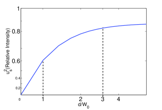
Figure 3: (Color online) The scaled power spectral density of the random potential and the dimensionless factor $d/W_{0}$ in logarithmic coordinates. In the area of $0<d/W_{0}<1$ and $d/W_{0}>3$, the curve has a good linear fit.

The dependence between the strength of the random potential and $d$ can be assumed as

$$u_{s}=C(d)\cdot d^{-\alpha}$$ (11)

Based on the above analysis, the distance that the atoms lie above the wire $d$ have a linear fit in the logarithmic coordinates for the thin-line approximation when $d\gg W_{0}$ , so $C(d)$ is a constant describing the amplitude of the random fields, $\alpha$ the power index characterizing the speed the fields decays with $d$. The strength of the disorder potential drops with the growth of height $d$.

Using Eq.(8) and Eq.(11), we calculate $u_{s}$ for different $\xi$, and fit them against $d$ to get $\alpha$. The relationship between $\alpha$ and $\xi$ is plotted in Fig. 4. We can see the potential roughness decays with the height $d$ in direct relation to $\alpha$. As the correlation length $\xi$ increases, the index $\alpha$ decreases drastically. When $\xi$ is zero, $\alpha\rightarrow 2.5$, which is coincidental to the white-noise approximation. Provided that the deviation between the data from the experiment and theoretical calculation is mainly caused by the uncertainty of $\xi$, then in our calculations we elucidate the correlation length of the system, i.e., the fluctuation of the edge of the wire should be a finite number on a large scale. For instance, the correlation length in experiments Kraft ; Esteve should be $75\mu m$ pointed out by our figure as well as further calculations. The power index $\alpha$ is determined as soon as $\xi$ is determined.

The strength factor $\sigma^{2}$ in the colored-noise correlation function Eq.(9) only contributes to the constant before the integral in Eq.(7) and is totally not relevant to the shape of the random potential, so it has no effect on the power index $\alpha$. However we can see below its influence on the density profile is similar to the alteration of the distance $d$.

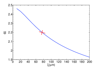
Figure 4: (Color online) Relationship between the power index $\alpha$ and the correlation length $\xi$ in the case of thin-line approximation ($d\gg W_{0}$). The cross point is the typical value $\xi=75\mu m$ and $\alpha=2.2$.

IV THE FORM OF ROUGH POTENTIAL AND FLUCUATIONS OF THE DISTRIBUTION

We then discuss the disturbance of the distribution of BEC atoms caused by the random magnetic fields. The rough potential in the trap can be obtained in experiments by measuring the density profile of cold atom clouds via absorption imaging method. As the BEC atoms expand mainly in the z-direction, and are very tight in the other two dimensions, the distribution can be described by the one-dimension Gross-Pitaevskii Equation(GPE) Dalfovo

$$i\hbar\frac{\partial\Psi}{\partial t}=-\frac{\hbar^{2}}{2m}\nabla^{2}\Psi+V(z)\Psi+NU_{0}\left|\Psi\right|^{2}\Psi$$ (12)

$\Psi$ satisfies the unitary normalization condition, $N$ is the number of BEC atoms and $U_{0}=4\pi\hbar^{2}a/m$ is the intensity of mean field interaction. $V(z)$ includes both harmonic potential and the fluctuated potential as follows Bao

$$V(z)=\frac{1}{2}m\omega_{z}^{2}z^{2}+V_{d}(z).$$ (13)

$V_{d}(z)$ is the random potential induced by the fluctuation, and $\omega_{z}$ is the frequency in the z-direction. Here we use a method similar to Modugno to generate a random potential with desired correlation function.

$$V_{d}(z)=\mathcal{F}^{-1}[W(k)\mathcal{F}[g(z)]],$$ (14)

where $W(k)$ is a an appropriate aperture function which can filter out high and low part of the signal. With $V_{d}(z)$ we use backward euler finite difference (BEFD) to compute the dynamic evolution of the GPE and finally get the wave function $\Psi$ and the density profile $|\Psi|^{2}$ Bao .

Due to the random potential induced by the fluctuation of the magnetic fields, a series of fragmentations in the condensate density profiles come into being. For different bias field values, the experimental sequence used to produce ultra-cold atoms in this trap were carried out, corresponding to different distances from the magnetic trap to the top surface of the wire. The strength of the random potential is mainly affected by the value $\sigma^{2}$ in Eq.(9). When the strength is relatively large, the random potential is comparable to the harmonic potential. The fragments present a high peak, and the density distribution rises and falls sharply, as shown in Fig. 5.

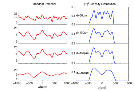
Figure 5: (Color online) Density profile of the BEC atoms and the random potential at different heights on the case of large random potential. The left column indicates the random potential at 50$\mu m$, 100$\mu m$, 150$\mu m$ and 200$\mu m$ respectively from top to bottom. The right column is for the normalized distribution $|\Psi|^{2}$ at the height of 50$\mu m$, 100$\mu m$, 150$\mu m$ and 200$\mu m$ from top to bottom. Figures for $|\Psi|^{2}$ range the same from 0 to 0.2. $\xi$ is fixed at $75\mu m$. Kraft

Fig. 6 shows effect of the disorder strength on the density profile. We focus on the area around the main peak and take out the $1000\mu m$ area. The relative roughness strength in Fig. 6 (a-d) is 1:2:6:10. From the figure we can see the fragmentation gradually becomes obvious as the strength increases. At the appropriate strength for the random potential, as shown in Fig. 6(c), the density profile basically coincides with the experiment Kraft . The amplitude for the fragments are different with one highest and others decreasing accordingly, and the distance between two peaks in the $1000\mu m$ area is about $250\mu m$. The characteristics of the experiment Kraft are reflected by our calculations.

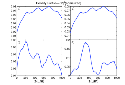
Figure 6: (Color online) Effect of the disorder strength on the density profile with $\xi=75\mu m$. The relative strength in (a), (b), (c) and (d) is 1:2:6:10.

First we discuss the effects of height $d$ at a finite correlation length $\xi$. We can see the dependence between the random potential and the distance in the left column of Fig. 5. It indicates the random potential at 50$\mu m$, 100$\mu m$, 150$\mu m$ and 200$\mu m$. The right column is for the density distribution. Using the equation $u_{s}^{2}=Cd^{-2.2}$ given above, we can assess the strength of the potential quantitatively. As the distance increases, the roughness of the random potential weakens. Meanwhile the fragmentation phenomenon in the density distribution becomes less obvious.

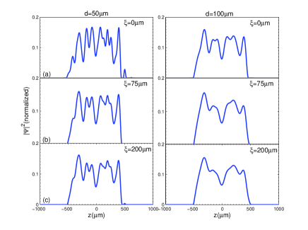
Figure 7: (Color online) The normalized density profile of the BEC atoms for different correlation length. The left column for the height $d=50\mu m$. The right column for $d=100\mu m$. All the figures have the same range for $|\Psi|^{2}$ from 0 to 0.2. (a) $\xi=0\mu m$ (b) $\xi=75\mu m$ (c) $\xi=200\mu m$.

Then we show the influence of different correlation length at a fixed height $d$. Fig. 7 demonstrates how the correlation length of the system affects the distribution of BEC atoms. The left column is for different correlation lengths 0$\mu m$, 75$\mu m$, 200$\mu m$ at the height $d=50\mu m$, and the right column is for all the same conditions except for $d=100\mu m$. When the system has an intrinsic correlation length, the fragmentation of the density profile is apparently small than that of the white noise. In two extreme cases, as $\xi\rightarrow\infty$, the distribution becomes smooth because it is the ideal situation that the current-carrying wire has no fluctuation, while $\xi\rightarrow 0$ is the simple white-noise case, and the fluctuation is at its maximum. We are most interested in Fig. 6(c) when $d=100\mu m$ and $\xi=75\mu m$. This set of data is measured in the experiment Kraft . The number of the fragmentations, which is about 4 along the z-axis over $1000\mu m$, is in good agreement with the image derived from the experiment, better than that of the white-noise approximation (about 6) which is different from the experimental data.

V DISCUSSION AND CONCLUSION

According to our analysis, different correlation length will lead to different $\alpha$. As in experiment Kraft ; Esteve , $\alpha=2.2$, the plausible correlation length through our calculations, should be $75\mu m$, and the density profile we thus get is coincidental with the experiment. The spectral density of the distribution Esteve shows that $\xi$ has a very small fluctuation $100nm$, so the features of a system could be considered as a finite correlation length. We also take the width of the wire into account, pointing out exactly how it affects the random potential. Though the real trap is not a thin-wire, our model indicates when the height $d$ is relatively large, it is rational to ignore the width of the wire. We then analyze how the strength of the random potential affects the density distribution. The density profile for the appropriate disorder strenth in our theoretical picture is in better accordance than the previous white-noise approximation to some extent, which proves our conclusions to be more reasonable. That is to say, by counting the number of fragmentations of the atoms, we can see qualitatively the correlation length of the wire. By furthermore measuring the power spectral density of the disorder potential, we can get the correlation length quantitatively.

In summary, we bring forth a more general model to calculate the random potential for the BEC atoms in a current-carrying wire. We show that the fluctuation in the potential is caused by the distortion of the wire edge with a fixed correlation length. The correlation length of the specific wire used in experiment Kraft is $\xi=75\mu m$ and the power index in $u_{s}=C\cdot d^{-\alpha}$ is $2.2$. This might be applicable in the precise measurement because of the possible criterion provided for the necessary wire quality to be used for cold atom manipulation. Besides, by measuring the spectral density of cold atom distribution and analyzing the deviation in the data we get from theoretical calculations and experiment, we can get to know the nature of the noise, and apply it in the simulation of the transport process.

VI ACKNOWLEGEMENT

X. J. Zhou thanks to E. A. Hinds, B. Darquie and H. T. Yin for their help and discussion. This work is partially supported by the state Key Development Program for Basic Research of China (No.2005CB724503, 2006CB921401, 2006CB921402), and by NSFC (No.10874008 and 10934010).

References

- (1) R. Folman, P. Kruüger, J. Schmiedmayer, J. Denschlag, and C. Henkel, Adv. At. Mol. Opt. Phys.48, 263 (2002).
- (2) J. Fortágh and C. Zimmermann, Rev. Mod. Phys. 79, 235 (2007).
- (3) W. Hänsel et al., Nature (London) 413, 498 (2001).
- (4) A. E. Leanhardt, Y. Shin, A. P. Chikkatur, D. Kielpinski, W. Ketterle, and D. E. Pritchard, Phys. Rev. Lett. 90, 100404 (2003).
- (5) D. W. Wang, M. D. Lukin, and E. Demler, Phys. Rev. Lett. 92, 076802 (2004).
- (6) T. Schumm, J. Estve, C. Figl, J. B. Trebbia, C. Aussibal, H. Nguyen, D. Mailly, I. Bouchoule, C. I. Westbrook and A. Aspect, Eur. Phys. J. D 32, 171 (2005).
- (7) S. Kraft, A. G nther, H. Ott, D. Wharam, C. Zimmermann and J Fortágh, J. Phys. B: At. Mol. Opt. Phys. 35, L469 (2002).
- (8) G. Palasantzas, Phys. Rev. B 48, 14472 (1993).
- (9) Z. Moltadiry, B. Darquire, M. Krafty, E. A. Hinds, Jour. Mod. Opt. 54, 2149 (2007).
- (10) X. J. Zhou, Phys. Rev. A 80, 023818 (2009).
- (11) J. Esteve, C. Aussibal, T. Schumm, C. Figl, D. Mailly, I. Bouchoule, C. I. Westbrook and A. Aspect, Phys. Rev. A 70, 043629 (2004).
- (12) F. Dalfovo, S. Giorgini, L. P. Pitaevskii, S. Stringari, Rev. Mod. Phys. 71 ,463 (1999).
- (13) W. Bao, D. Jaksch and P. A. Markowich, J. Phys. 187, 318 (2003).
- (14) M. Modugno, Phys. Rev. A 73, 013606 (2009).
- (15) Jun S. Liu, Monte Carlo Strategies in Scientific Computing, Springer.