Fuzzy Supernova Templates II: Parameter Estimation

Abstract

Wide field surveys will soon be discovering Type Ia supernovae (SNe) at rates of several thousand per year. Spectroscopic follow-up can only scratch the surface for such enormous samples, so these extensive data sets will only be useful to the extent that they can be characterized by the survey photometry alone. In a companion paper (Rodney and Tonry, 2009) we introduced the SOFT method for analyzing SNe using direct comparison to template light curves, and demonstrated its application for photometric SN classification. In this work we extend the SOFT method to derive estimates of redshift and luminosity distance for Type Ia SNe, using light curves from the SDSS and SNLS surveys as a validation set. Redshifts determined by SOFT using light curves alone are consistent with spectroscopic redshifts, showing a root-mean-square scatter in the residuals of $RMS_{z}=0.051$. SOFT can also derive simultaneous redshift and distance estimates, yielding results that are consistent with the currently favored $\Lambda$CDM cosmological model. When SOFT is given spectroscopic information for SN classification and redshift priors, the RMS scatter in Hubble diagram residuals is 0.18 mags for the SDSS data and 0.28 mags for the SNLS objects. Without access to any spectroscopic information, and even without any redshift priors from host galaxy photometry, SOFT can still measure reliable redshifts and distances, with an increase in the Hubble residuals to 0.37 mags for the combined SDSS and SNLS data set. Using Monte Carlo simulations we predict that SOFT will be able to improve constraints on time-variable dark energy models by a factor of 2–3 with each new generation of large-scale SN surveys.

The use of Thermonuclear Supernovae (TN SNe, i.e. Type Ia SNe) as cosmological standard candles requires the determination of each SN’s redshift and distance modulus. This has traditionally been done with two parallel measurements: a spectrum confirms the object’s class and provides a very accurate redshift, while a broad band light curve allows the estimation of luminosity distance. Technological advances in wide-field imagers are now opening the door for a new generation of large area surveys. Projects such as the Palomar Transient Factory (PTF; Rau et al., 2009; Law et al., 2009), and Pan-STARRS 1 (PS1; Kaiser et al., 2002) are already beginning to amass SN samples that will eventually number in the thousands. In coming years Pan-STARRS 4, LSST, and JDEM will uncover tens of thousands of SNe. From these vast collections of SN light curves, only a small fraction will be spectroscopically observed, meaning that any analyses applied to them will have to rely on photometry alone.

In Rodney & Tonry (2009) (hereafter Paper I), we introduced SOFT (Supernova Ontology with Fuzzy Templates) and described in detail the structure and form of the SOFT light curve analysis method. In this paper, Section 1 begins with a brief review of the basis for the SOFT method and the fuzzy set theory framework for light curve comparisons. In Section 2 we apply the SOFT models to the task of estimating cosmological parameters using SN light curves. Verification tests using data from the Sloan Digital Sky Survey (SDSS) and the Supernova Legacy Survey (SNLS) are described in Section 3. The results of these tests are then extended to produce Monte Carlo simulations of future surveys to examine how well an approach such as SOFT will be able to constrain dark energy models. A discussion of the inherent biases in our template estimators is provided in Section 5, and a summary of results is presented in Section 6.

1 Light Curve Models

The shape of an observed SN light curve can be described by two sets of parameters. The first set, which we denote ${\bf\Phi}$, consists of all relevant physical parameters that determine the intrinsic shape and color of the light curve (e.g. the ${}^{56}\mbox{Ni}$ mass, the degree of mixing in the stellar interior, etc.). A second set of parameters, $\theta$, relate to the location of the SN in space and time: redshift $z$, luminosity distance $\mu_{e}$, host galaxy extinction A_V, and time of peak t${}_{\mbox{\tiny pk}}$. These four location parameters modify the intrinsic light curve shape by stretching and dimming it into the form that we eventually observe.

We do not have a complete physical model for SN explosions that could efficiently and reliably translate a vector of physical parameters ${\bf\Phi}$ into a precise light curve prediction. Therefore, most TN SN light curve fitters – such as MLCS (Riess et al., 1996; Jha, 2002) and SALT (Guy et al., 2005, 2007) – use one or more paramaters (e.g. $\Delta$, or X1 and C) to define the shape and color of a broad-band SN light curve. By contrast, the SOFT method has no shape or color parameters, but instead uses a collection of SN light curve templates to provide examples of possible shapes and colors. These template light curves are then warped to reproduce the effects of a change in location $\theta$. By comparing this adapted light curve model against a candidate SN object, we can derive the likelihood that the candidate has an intrinsic light curve shape similar to the template, and is at the assumed location $\theta$.

In Paper I we discussed how our template-based approach is best served by utilizing the framework of fuzzy set theory (Zadeh, 1965), and we applied SOFT to the task of SN classification. In this paper we will now explore how the application of fuzzy logic allows us to extend the SOFT method to the problem of estimating cosmologically useful parameters such as a SN’s redshift and distance.

2 Parameter Estimation

Suppose we have a candidate object called SN X whose observed light curve is given by a series of points $D_{i}=(t_{i},f_{i},\sigma_{i})$. Here $t_{i}$ is the observation time, $f_{i}$ is the measured flux, and $\sigma_{i}$ is the uncertainty for epoch $i$. The complete light curve with N data points is denoted by the vector ${\bf D}$. If we assume a set of location parameters $\theta$ then a light curve model $M_{j}$ that realizes a given ${\bf\Phi}$ provides a prediction for a SN’s flux as a function of time: $\mathcal{F}_{j}(t_{i},\mbox{\boldmath$\theta$})$.

In the framework of traditional probability theory, we would describe the probability of observing the data ${\bf D}$ given model $M_{j}$ and location $\theta$ as the combined probability of the data-minus-model error terms:

$$p({\bf D}|\mbox{\boldmath$\theta$},M_{j})=\prod\limits_{i=1}^{N}\frac{1}{\sqrt{2\pi}\sigma_{i}}\mbox{exp}\left(\frac{-(f_{i}-\mathcal{F}_{j}(t_{i},\mbox{\boldmath$\theta$}))^{2}}{2\sigma_{i}^{2}}\right)$$ (1)

(see Equations 4-6 in Paper I). We then compute the probability that our candidate object resides at any particular location $\theta$ by applying Bayes theorem:

$$p(\mbox{\boldmath$\theta$}|{\bf D},M_{j})=\frac{p(\mbox{\boldmath$\theta$}|M_{j})~{}p({\bf D}|\mbox{\boldmath$\theta$},M_{j})}{\int\limits_{\theta}{p(\mbox{\boldmath$\theta$}|M_{j})~{}p({\bf D}|\mbox{\boldmath$\theta$},M_{j})~{}~{}d\mbox{\boldmath$\theta$}}}$$ (2)

This gives us a probability distribution over the four dimensions of $\theta$, under the assumption that our candidate SN X is physically identical to the model $M_{j}$. Variations of this approach using parameterized light curve models have been applied to SN classification (Sullivan et al., 2006; Johnson & Crotts, 2006; Kuznetsova & Connolly, 2007; Poznanski et al., 2007) as well as to the estimation of SN redshifts (Barris & Tonry, 2004; Kim & Miquel, 2007; Gong et al., 2010).

With SOFT, however, we remove the need for a parametric model of the SN light curve by limiting ourselves to a finite set of fixed-shape models. To keep within the framework of traditional probability theory, we could apply Equation 2 to derive probabilities from all our models and then combine the results using a method such as Bayesian Model Averaging (Hoeting et al., 1999). Unfortunately, that approach is applicable only in the case where our set of models is complete and non-redundant. If either of those two conditions is not satisfied, then the normalization inherent in applying Bayes’ theorem is not valid. In Paper I we have argued that it is impossible to completely satisfy both conditions when using a finite library of fixed-shape templates.

2.1 Biased Estimators

In addition to problems of logical incongruence described above and in Paper I, our finite set of templates will necessarily introduce an element of bias to any parameter estimates. To illustrate this problem, suppose we have an extremely sparse template library, consisting of only two template models, $M_{1}$ and $M_{2}$. Now let us observe a candidate object, SN X, which has physical parameters ${\bf\Phi}$_X that are intermediate between ${\bf\Phi}$₁ and ${\bf\Phi}$₂ (e.g., perhaps the candidate has a ${}^{56}\mbox{Ni}$ mass that is bracketed by the two templates: $M_{Ni,1}<M_{Ni,x}<M_{Ni,2}$). SN X is not a perfect match with either of the two models, so applying Eq. 2 will give us a biased parameter estimate from each of them. For simplicity suppose that all the location parameters are fixed except for the cosmological dimming, $\theta$$=$$\mu_{e}$. The model $M_{2}$ with a higher $M_{Ni}$ will have a higher bolometric flux than SN X (Arnett, 1982). Thus, the best match from the $M_{2}$ model will have to increase the cosmological dimming $\mu_{e}$ away from the true value to compensate. Conversely, the fainter $M_{1}$ model must decrease the cosmological dimming (lower $\mu_{e}$ $\rightarrow$ higher flux) to bring it up to the level of SN X. Therefore $M_{1}$ will report a lower $\mu_{e}$ as the most likely parameter.

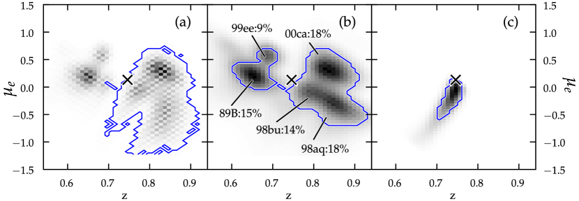
Figure 1: Demonstration of the parameter estimation biases inherent in a finite set of light curve templates, and the bias averaging enabled by fuzzy templates. The candidate SN used here was the SNLS object 04D2ja. (a) Probability distributions constructed using the strict Bayesian approach of Equations 1 and 2 (i.e. without any model fuzziness). The ‘x’ marks the spectroscopic redshift of this SN and the corresponding distance modulus for a universe with $H_{0},\Omega_{M},\Omega_{\Lambda}=(70,0.3,0.7)$. The gray-scale shading defines the probability distribution, and the contour line encloses the region about the peak that contains 68% of the probability. (b) The introduction of model fuzziness using $\sigma^{\prime}_{j}$ as in Section 2.2 expands the area of parameter space in which each model can provide a fair match. For this candidate SN, our template library finds 5 templates that provide reasonable fits. Here we display the “probability” cloud that defines each individual fuzzy set membership function, simply summing them together without using a proper fuzzy set combination operator. Each cloud is marked with the designation of its generating template and a percentage that indicates its integrated membership grade $\gamma$ (Eq. 5). (c) After rejecting outliers with a membership cut at 5%, we combine the remaining fuzzy membership functions using the Dombi intersection operator. This “Fuzzy AND” operation tends to average out the biases of any individual template.

In Figure 1a we illustrate this parameter bias using a real SN light curve from the SNLS, the Type Ia SN 04D2ja. We compared this object’s light curve against all 28 TN SN templates, in each case using equation 2 to construct a probability distribution in the z-$\mu_{e}$ plane. The sum of these distributions, shown in Figure 1a, is diffuse and inaccurate, with multiple peaks spread across the parameter space. No individual template provides a clear match to the shape of the candidate light curve, so each template requires an offset from the true location in order to compensate for the shape mismatch.

2.2 Fuzzy SN Models

We now have two problems arising from the traditional (Bayesian) approach to parameter estimation when using a finite set of templates. First is the problem of violating the assumptions of completeness and non-redundancy (see section 4 of Paper I), and second is the issue of parameter estimation biases described above. We propose that both of these problems are resolved by invoking fuzzy logic, an alternative logical framework that is better suited to the case of our limited template library.

In Paper I we developed the basic structure of a fuzzy SN model. Each template model $M_{j}$ carries an associated “model fuzziness” term, $\sigma^{\prime}_{j}$, which is used to define a fuzzy set around that template. The $\sigma^{\prime}_{j}$ term quantifies how membership in that model’s fuzzy set falls off as light curves become more and more dissimilar to the template curve:

$$\begin{array}[]{ll}p^{\prime\prime}({\bf D}|\mbox{\boldmath$\theta$},M_{j})=&\prod\limits_{i=1}^{N}{\frac{1}{\sqrt{2\pi}\sqrt{\sigma_{i}^{2}+{\sigma^{\prime}_{j}}^{2}}}}\\ &\times\ \mbox{exp}\left(\frac{-\left(f_{i}-\mathcal{F}_{j}(t_{i},\theta)\right)^{2}}{2~{}(\sigma_{i}^{2}+{\sigma^{\prime}_{j}}^{2})}\right)\\ \end{array}$$ (3)

(cf. Eq. 1 and Paper I, Eq. 13).

It is no accident that this expression for the likelihood is functionally identical to what we would use in traditional probability theory if $\sigma^{\prime}_{j}$ was a simple model uncertainty. There is a conceptual difference between the two types of uncertainty: our model fuzziness represents an intentional “vagueness” or “indefiniteness,” whereas the traditional model uncertainty encapsulates an “imprecision” or “inaccuracy.” In the language of set theory, our fuzzy model defines a set that includes “All SNe that are physically similar to model $M_{j}$.” This leaves room for our model to be applied to objects that we know to be slightly different from our template. By contrast, in traditional probability theory a model $M_{j}$ defines a set that includes “All SNe that are physically identical to model $M_{j}$,” and the addition of model uncertainty would simply acknowledge that we don’t know exactly what our model $M_{j}$ really looks like. Although the mathematical form is the same, the fuzzy concept of vagueness allows us to adjust the strength of $\sigma^{\prime}_{j}$ to suit our purposes (increasing $\sigma^{\prime}_{j}$ makes the model more inclusive but less predictive), whereas a traditional model uncertainty should be derived strictly from empirical evidence. As we will see in the next section, this model fuzziness also leads us to a powerful advantage within fuzzy logic, namely that we can apply a fuzzy AND combination instead of the less informative OR.

To convert the likelihood of Equation 3 into a fuzzy membership grade we introduce a prior on the location parameters, $p(\mbox{\boldmath$\theta$}|M_{j})$, as well as a prior for the particular template in question, $p(M_{j})$. The final membership grade for our candidate SN X in the ($\theta$,$M_{j}$) fuzzy set is given by:

$$g({\bf D}|\mbox{\boldmath$\theta$},M_{j})=p(\mbox{\boldmath$\theta$}|M_{j})~{}p(M_{j})~{}p^{\prime\prime}({\bf D}|\mbox{\boldmath$\theta$},M_{j})$$ (4)

(see Paper I, Eq. 14 and section 5.1 for a full description of fuzzy membership functions).

To compare the quality of fit between two or more models, we define a scalar quantity $\gamma$ as a normalized integral over the location parameters $\theta$. For a single model $M_{j}$ we have:

$$\gamma_{j}=\frac{\int\limits_{\theta}{g({\bf D}|\mbox{\boldmath$\theta$},M_{j})}\delta\theta}{\sum\limits_{k}~{}\int\limits_{\theta}{g({\bf D}|\mbox{\boldmath$\theta$},M_{k})}\delta\theta}$$ (5)

where the summation is over all available models. The value of $\gamma_{j}$ lies in the range [0,1] and measures the candidate object’s strength of association with model $M_{j}$ relative to all other models. This term can serve as the fuzzy analog for a Bayesian posterior probability.

By adding an element of fuzziness to the SN models, we have alleviated the logical inconsistencies of the Bayesian approach when applied to our finite template library (see section 4.1 of Paper I). We have not, however, removed the inherent biases in the parameter estimates of individual templates. Returning to our example from the SNLS, in Figure 1b we show a stack of membership functions from comparison of the candidate SN against our fuzzy TN SN models. The five most prominent membership function clouds are labeled with the templates they originate from as well as a percentage showing the value of $\gamma$ from Equation 5. The addition of model fuzziness has smoothed the peaks of the distribution, but individual membership functions are still biased by the mismatch of light curve shape between our candidate and the templates. We would like to be able to combine these membership functions together in a way that gives us an improved composite parameter estimate. In the following section we explore how this can be achieved using the structures of fuzzy logic.

2.3 Fuzzy Combination

The two principle operators for fuzzy logic can be defined in a number of ways. As described in the companion paper, we have adopted the Dombi (1982) operators (see Paper I, Section 5.2, Equations 16 and 17), which define how two fuzzy membership functions can be combined in a logical intersection (fuzzy AND) or union (fuzzy OR). To choose whether to use the intersection or the union operator for our SN models we must consider how much interaction between the fuzzy sets is appropriate for the problem.

Suppose we have done two model comparisons, using models $M_{1}$ and $M_{2}$ to get two membership functions $g_{1}=g({\bf D}|\mbox{\boldmath$\theta$},M_{1})$ and $g_{2}=g({\bf D}|\mbox{\boldmath$\theta$},M_{2})$. Let us also suppose that these two models are based on SNe that have intrinsically very similar physical characteristics: ${\bf\Phi}_{1}\sim{\bf\Phi}_{2}$. If it happens that our candidate SN X has underlying physical parameters ${\bf\Phi}$_X that are similar to both ${\bf\Phi}$₁ and ${\bf\Phi}$₂, then we should expect that the location parameter estimates from those two models should strongly agree. That is, the location parameter biases from these two models should be small enough that the true location of our candidate, $\theta$_X, will be simultaneously favored by both $M_{1}$ and $M_{2}$. This argues for the use of the intersection operator (Paper I, Eq. 17) when combining $g_{1}$ with $g_{2}$.

Now suppose that we carry out a third model comparison with model $M_{3}$, and let us assume that this model has intrinsically very different physical parameters ${\bf\Phi}$₃. The larger separation between ${\bf\Phi}$₃ and ${\bf\Phi}$_X means that the light curve shapes of $M_{3}$ and SN X will be substantially different, and therefore $M_{3}$ will have to introduce a large $\theta$ bias in order to compensate. In this case, we should expect that the intersection of $g_{3}=g({\bf D}|\theta,M_{3})$ with either $g_{1}$ or $g_{2}$ will not provide a useful estimate of the true candidate location. Thus, an intersection operation would give misleading results, as the outlier $g_{3}$ pulls the composite membership distribution away from the real value of $\theta$_X.

If we expect that template mismatches such as $M_{3}$ are included in the group of membership functions being combined, then we cannot justify using the fuzzy AND operator. If, however, we can exclude those outliers from our combination group, then the intersection operation is justified, and should provide a more precise estimate of $\theta$_X. The $\gamma$ value provides a simple (though somewhat crude) metric for this purpose. We can exclude templates that have very different light curve shapes from our candidate by rejecting any models that yield a $\gamma$ value below some threshold. For the validation tests described in the following section we have used a cutoff of $\gamma<5\%$.

In Figure 1c we show the end result of applying the fuzzy AND operation to combine membership functions for the SNLS object 04D2ja. The resulting composite membership function has a single peak in the region that all models collectively agree upon as a likely location for the candidate SN. In the case of 04D2ja, the parameter estimate from this intersection of membership functions provides a better estimate than any single light curve template could provide. This is true because each individual template has a location parameter bias that attempts to compensate for the mis-match in light curve shape. The length and direction of these bias vectors are distributed more or less randomly over the space of $\theta$. Thus, when many models are combined together the biases tend to cancel out. It is important to note that if we had not used the crude 5% threshold to cut out severe mismatches, then a few of the models that are most egregiously biased would have dominated the intersection operation, pulling the combined distribution off into a distant corner of $\theta$ space. In Section 5 we will discuss a possible method of calibrating the template library that could alleviate the need for this threshold cut.

3 Verification Tests

3.1 Data Sets

Table 1: Verification Data Subsets

Data set	$N_{SNe}$	Description
SDSS-A	145	all SNe from Holtzman et al. (2008) except SN05gj (unfittable)
SDSS-B	127	photometric cut : -10 classified by SOFT as CC; -8 with one-sided light curves
SDSS-C	116	photo-cut + spec. cut : -11 with spectroscopic classification “Ia?”
SNLS-A	71	all 71 SNe from Astier et al. (2006)
SNLS-B	57	spectroscopic cut : -14 with spectroscopic classification “Ia*”
Combo	198	photometric cuts : union of SDSS-B with SNLS-A

To test the accuracy and precision of SOFT estimates for $z$ and $\mu_{e}$, we used a combination of data from the SDSS-II and SNLS programs. We use 146 spectroscopically confirmed Type Ia SNe from Holtzman et al. (2008) and 71 from the SNLS project (Astier et al., 2006). The SDSS sample spans a redshift range from 0.01 to 0.45, while the SNLS SNe fall between 0.25 and 1.0. From this combined data set of 217 SNe, we have extracted a series of subsets that attempt to eliminate objects that are most problematic for light curve analysis with SOFT. Table 1 lists the six subsets used.

The SDSS-A subset rejects only one singularly peculiar object, SN2005gj. We define the SDSS-B sample using photometric selection criteria: excluding ten objects that are classified as core collapse SNe by SOFT (see Paper I for details on the classification procedure), and eight objects that have one-sided light curves, lacking either the pre-peak or the post-peak epochs entirely. The final SDSS subset, SDSS-C, uses an additional cut to remove 11 more objects that were given a spectroscopic classification of “Ia?” by Holtzman et al. (2008), indicating some classification uncertainty.

The SNLS SNLS-A includes all 71 SNLS SNe presented by Astier et al. (2006). We do not apply a photometric cut to the SNLS data in the manner of SDSS-B, because SOFT classifies all 71 SNe as Type Ia, and the peak is well defined for all light curves. For the SNLS-B sample we exclude 14 objects that were given a “Ia*” classification in Astier et al. (2006) to indicate some classification ambiguity.

Our final data set is a combination of the photometrically selected samples from SDSS and SNLS. With 127 SNe from SDSS-B and 71 SNe from SNLS-A, the Combo subset contains 198 objects with complete light curves that SOFT recognizes as Type Ia.

3.2 Priors

For each SN in the verification data sets, we want to use Eq. 4 to define fuzzy set membership functions. To compute the location prior term in that equation, $p(\mbox{\boldmath$\theta$}|M_{j})$, we use flat uninformative priors for the parameters t${}_{\mbox{\tiny pk}}$ and $\mu_{e}$. For host galaxy extinction we apply the “Galactic Line of Sight” A_V prior employed by the ESSENCE team (Wood-Vasey et al., 2007), which is based on the host galaxy extinction models of Hatano et al. (1998), Commins (2004), and Riello & Patat (2005) (see Paper I, §3.1).

For the redshift prior we consider two alternative situations. In the first case, we assume a traditional SN survey strategy, where all SNe have spectroscopic measurements to define their redshifts and to aid in classification. The redshift prior for this scenario is based on the spectroscopic measurements reported by Holtzman et al. (2008) and Astier et al. (2006) for the SDSS and SNLS data sets, respectively. The prior is separately defined for each SN as a Gaussian centered on the measured redshift with width defined by $\sigma_{z}=0.005$. The parameter estimates that SOFT returns in this case can be more or less directly compared to the SN cosmology results elsewhere in the literature.

Our second redshift prior is designed to evaluate how well SOFT can measure redshift and distance without any spectroscopic information. As a worst case scenario we assume that there is no spectroscopic information available for any of the SNe or their host galaxies, and there are not even photometric redshift estimates from the host galaxies. For this case we want to use an uninformative redshift prior, reflecting our total ignorance of each object’s redshift. One possibility would be a flat distribution over $z$, normalized so that it integrates to unity over the range of redshifts under consideration for each SN candidate. A slightly more realistic prior would take into account the increasing volume of space as a function of redshift. For simplicity we assume a a flat $\Omega_{M}=0$ universe so that the volume of a shell at redshift z (per unit solid angle) is

$$p(z)dz\propto z^{2}dz$$

This is the uninformative prior that we use throughout this paper, although we also tested the flat z prior and found no significant changes in our conclusions.

3.3 Photometric Redshifts

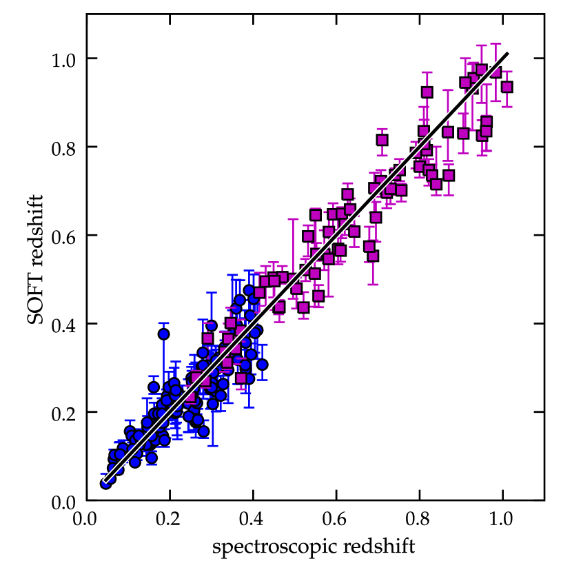
Figure 2: Comparison of the peak redshift estimates from SOFT against the spectroscopic redshift measurements from SDSS and SNLS. The SDSS SNe are plotted as (blue) squares, and SNLS objects are (magenta) circles. The solid line shows how the data would fall if SOFT photo-z’s traced the spectroscopic redshifts perfectly. The RMS scatter about the line is 0.048, and the reduced $\chi^{2}$ statistic is 1.51.

As a first test, we want to evaluate how well SOFT can determine a redshift based on the SN light curve alone. For this task we use the Combined data set, containing 198 photometrically identified Type Ia SNe from subsets SDSS-B and SNLS-A (see Table 1). Using the uninformative $z^{2}$ redshift prior, we determine a composite membership function from each TN SN model using Equation 4. The membership functions are marginalized over all nuisance parameters (A_V,t${}_{\mbox{\tiny pk}}$,$\mu_{e}$) and combined using the fuzzy AND operator to get a composite membership function over redshift: $g(z)$. We locate the peak of this distribution to define $z_{SOFT}$, and assign error bars by measuring the width of the contour that contains 68% of the area.

Figure 2 plots these SOFT redshift values against the spectroscopically measured redshifts from SDSS and SNLS. The residuals defined by $z_{SOFT}-z_{spec}$ have an RMS scatter about zero of 0.045 for the SDSS-A sample, 0.059 for SNLS-B, and 0.051 for the combined sample. The uncertainties for these data points are decidedly non-Gaussian and asymmetric. Nevertheless, the reduced $\chi^{2}$ term gives a rough measure of the accuracy of our uncertainty estimates, and we find $chi^{2}/DOF=$ 0.98, 1.25, and 1.08 for the SDSS-A, SNLS-B, and combined samples, respectively. These values being close to unity suggests that the SOFT error bars are accurately reflecting the true redshift uncertainties.

An appropriate comparison for these results is the work of Oyaizu et al. (2008), in which photometric redshift errors from $ugriz$ imaging of $\sim 300,000$ SDSS galaxies are evaluated across a similar range of redshifts. Oyaizu et al. found that the RMS scatter in photometric redshift errors ($\delta z=z_{phot}-z_{spec}$) for the set of all galaxies in their validation set was approximately 0.054. They also quantify the photo-z accuracy using $\sigma_{68}$, which measures the range of the $\delta z$ distribution that contains 68% of their validation set objects. The distribution of SDSS galaxy photo-z errors is more sharply peaked than a Gaussian distribution, but with larger tails. The $\sigma_{68}$ metric is less sensitive to the fat tails, so it shows a significantly tighter correlation to the spectroscopic redshifts, with $\sigma_{68}\approx 0.021$.

From this comparison we see that the galaxy photo-z’s and the SOFT light curve redshifts can be very complementary techniques for doing SN science without spectroscopy. Suppose a SN is detected and a galaxy is identified as a likely host. We can derive a photo-z from optical photometry of the host, and also determine a completely independent photometric redshift using SOFT analysis of the SN light curve. In most cases the galaxy photo-z will be more precise (i.e. it lies in the sharp peak of the photo-z residual distribution). However, if the photo-z error bar is large, then we should take that as evidence that the SOFT redshift is more reliable (i.e. the host photo-z may be a significant outlier, off in the fat tails of the residual distribution). If the photometric redshift of the presumed host galaxy strongly disagrees with the SOFT redshift, then we should be suspicious that the galaxy may be a chance superposition and may not actually be the SN’s host. Finally, in cases where the host galaxy is too faint for detection, the SOFT light curve redshift can serve as a reliable stand-in.

In practice, host galaxy photo-z’s can be fed into the SOFT program as a redshift prior, in exactly the same way as spectroscopic redshifts. SOFT will naturally balance that host galaxy prior against the posterior information provided by the SN light curve – just as it is done in purely Bayesian approaches. When using priors drawn from host galaxy redshifts (be they photometric or spectroscopic), some care must be taken to avoid introducing a redshift bias. If the redshift distribution of the galaxies is significantly different from the redshift distribution of the SN sample being studied, then the likelihood of chance superpositions is increased. For example, the photo-z catalog of Oyaizu et al. (2008) is primarily comprised of $z<0.4$ galaxies, so if that catalog were used to provide redshift priors for a survey like the SNLS then it would lead to underestimated redshifts for all the high-z SNe.

3.4 Photometric Cosmology

In addition to the photometric redshift verification test, we have also evaluated the ability of SOFT to provide simultaneous estimates of redshift and distance, for testing cosmological models. From each SDSS and SNLS light curve we derived a composite membership function in the (z,$\mu_{e}$) plane, in the manner depicted in Figure 1. From the resulting composite membership function, we extracted an estimate for z and $\mu_{e}$ by locating the peak of the composite membership function. To estimate the uncertainty we measured the height and width of the “1-$\sigma$ contour,” which we define as the border of the smallest contiguous region about the peak that contains 68% of the integrated value of the composite membership function. Figure 1c shows an example of the 1-$\sigma$ contour from a composite membership function.

In Figure 3 we show a Hubble diagram constructed with SOFT parameter estimates from all 146 SDSS SNe, using spectroscopic redshift priors. As described in the caption, different symbols indicate the objects that are excluded by photometric and spectroscopic cuts when culling down to the SDSS-A, B, and C subsets. Error bars have been withheld for clarity, so a representative error bar is shown in the lower right. Overlaid on the data points is a dashed line representing the $\Lambda$CDM cosmological model that is currently favored by observational data, with $H_{0}=70.5\,km\,s^{-1}$, $\Omega_{M}=0.273$, and $\Omega_{\Lambda}=0.726$ (Komatsu et al., 2009). Note that this model is presented here only as a metric for evaluating the SOFT results, and it was not generated by fitting to these data. Although the SOFT parameter estimates could be used to determine the best-fitting cosmological model for these particular data, such analysis is beyond the scope of this paper. The Hubble diagram in Figure 4 shows the SOFT results from all 71 SNLS SNe, also computed using spectroscopic redshift priors.

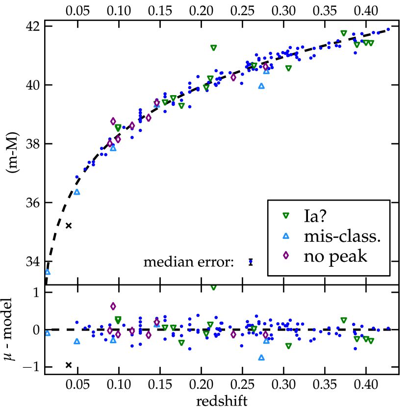
Figure 3: Hubble diagram showing SOFT parameter estimates from the SDSS verification data set, using spectroscopic redshift priors. All 146 of the SDSS-II SNe survey are plotted, with different symbols to indicate the classification cuts that define SDSS subsets A, B and C. Median error bars for $\mu_{e}$ are shown in the lower right. The 16 SNe with ambiguous spectroscopic classifications (the “Type Ia?” objects) are plotted as (blue) squares. The (cyan) triangles indicated 10 objects that SOFT classifies as Core Collapse SNe (5 of these are also in the “Ia?” set). An additional 8 objects that have one-sided light curves are plotted as (purple) diamonds. The X symbol marks SN 2005gj, a superluminous “Type IIa” object, which SOFT is unable to match with any Type Ia light curve. It is plotted at the position that SOFT would assign based on the best-fit template, which is the Type IIn SN 1994Y. In the lower panel we show the residual distance modulus values as a function of redshift. Goodness of fit statistics for the comparison of these data against the $\Lambda$CDM reference model are provided in Table 2.

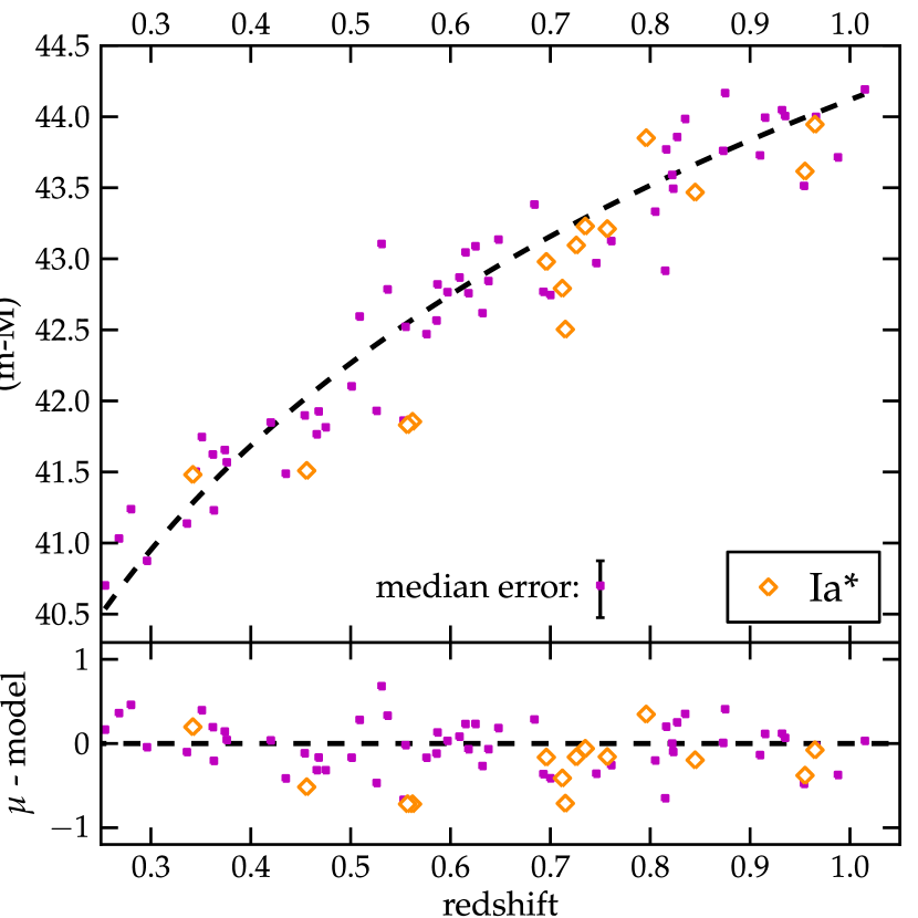
Figure 4: Hubble diagram showing SOFT parameter estimates of the SNLS verification data set, as in Fig. 3. For 14 objects with uncertain spectroscopic classifications (the “Type Ia*” SNe) we plot (magenta) squares. A median error bar is shown in the lower right, and residuals are plotted in the lower panel. Goodness of fit statistics from the comparison of these data against the $\Lambda$CDM reference model are given in Table 2.

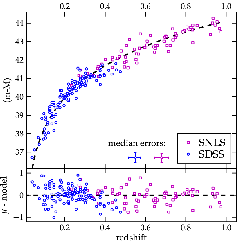
Figure 5: Hubble diagram from the Combined verification data set (see Table 1). All redshifts and distances are derived by SOFT alone, using the uninformative $z^{2}$ redshift prior. Objects with one-sided light curves and those which SOFT classifies as core collapse SNe have been rejected, but no spectroscopic classification cuts were used. Goodness of fit statistics from a comparison against the $\Lambda$CDM reference model are shown in Table 2.

To quantify the comparison of our SOFT parameter estimates against the Komatsu et al. 2009 model, we compute the $\chi^{2}$ goodness-of-fit statistic. For the distance modulus uncertainty we use the quadratic sum of the positive and negative $\mu_{e}$ uncertainties and a redshift uncertainty component:

$$\sigma_{\mu}^{2}=\sigma_{\mu,{\rm pos}}^{2}+\sigma_{\mu,{\rm neg}}^{2}+\sigma_{\mu,z}^{2}$$ (6)

For simplicity, we have projected the redshift uncertainty of each object onto the $\mu_{e}$ axis using

$$\sigma_{\mu,z}^{2}=\sigma_{z}^{2}\left(\frac{5}{ln(10)}\right)\frac{(1+z)}{z(1+z/2)}$$ (7)

in which $\sigma_{z}^{2}=\sigma_{z,{\rm pos}}^{2}+\sigma_{z,{\rm neg}}^{2}$ is the quadratic sum of positive and negative redshift errors derived from the 1$\sigma$ contours.

In addition to the reduced $\chi^{2}$ test, we measure the scatter about the model by computing the root mean square Hubble residual values:

$$RMS_{\mu}=\sqrt{\frac{\sum\limits_{i}(\mu_{e}^{SOFT}-\mu_{e}^{model})^{2}}{N}}$$ (8)

where $N$ is the number of SNe in the sample. A summary of these fit quality statistics for all data subsets is provided in Table 2.

Table 2: Hubble Diagram : Goodness of Fit Statistics

data set	$\chi_{\mu}^{2}$	$N_{DOF}$	$\chi^{2}/N$	RMSμ
with spectroscopic priors
SDSS-A	504.5	142	3.55	0.23
SDSS-B	398.3	124	3.21	0.21
SDSS-C	178.1	113	1.58	0.18
SNLS-A	135.8	68	1.99	0.31
SNLS-B	93.5	54	1.73	0.28
no spectroscopic information
SDSS-A	272.8	142	1.92	0.43
SDSS-B	141.1	124	1.14	0.38
SNLS-A	96.4	68	1.42	0.35
Combined	238.5	195	1.22	0.37

We can see from Figures 3 and 4 and from Table 2 that the photometric and spectroscopic cuts are doing a good job of removing serious outliers: the $\chi^{2}$ and $RMS$ statistics improve each time a set of suspect SNe is removed. When spectroscopic redshift priors are included, the RMS scatter from SOFT approaches the precision that can be achieved with other light curve fitters. As a recent example, Kessler et al. (2009) applied MLCS2k2 and SALT-II to approximately the same data. Using 103 objects from the SDSS sample (comparable to our SDSS-C subset), Kessler et al. found $RMS_{\mu}=0.15$ mags when using MLCS2k2. With 62 SNe from the SNLS sample (similar to our SNLS-B), they get $RMS_{\mu}=0.24$ mags.

As is to be expected, when SOFT has no spectroscopic information to use for weeding out misclassifications and for defining redshift priors, the resulting fit statistics are degraded. However, even with no spectroscopic help, SOFT is still able to produce consistent and reliable redshift and distance estimates across the entire range of z. The spectroscopy-free Hubble diagram of Figure 5 shows that the increased RMS scatter is not being driven by large systematic shifts. The fact that reduced $\chi^{2}$ statistics in the lower half of Table 2 are close to unity indicates that the SOFT uncertainty estimates are doing a good job of representing the true error in the z and $\mu_{e}$ parameter estimates. Recall that our redshift priors for this spectroscopy-free cosmology test were constructed under the assumption of a “worst-case scenario,” with no host galaxy photo-z estimates at all. In reality, many SNe from future wide-field surveys will have good photometric redshifts from their host galaxies, which can significantly improve the SOFT parameter estimates. Those future wide-field surveys will also have much larger data samples, helping to reduce the parameter estimate uncertainties that arise from random effects. As the sample size increases, however, systematic uncertainties will begin to dominate. In Section 5 we will consider potential modifications of the SOFT method that may help to minimize systematic errors.

4 Variable Dark Energy

One of the primary reasons for developing a tool such as SOFT is to deal with the extremely large SN data sets from a new generation of synoptic surveys. A principal science goal for these next generation surveys is to improve constraints on a time-variable dark energy (DE) equation of state. In this section we ask: How much of an improvement can be made with the precision provided by SOFT?

As a foundation for our simulations we must first adopt a DE model in which the equation of state parameter, $w$, is a function of the scale factor $a$, and therefore varies over cosmic time. A simple and commonly used parameterization for $w(a)$ is to assume a linear form (Chevallier & Polarski, 2001; Linder, 2003):

$$w(a)=w_{0}+w_{a}(1-a)$$ (9)

For our simulations we add the additional restriction of a flat universe ($\Omega_{\mbox{\scriptsize k}}$=0). The Friedmann equation in this case is:

$$\begin{array}[]{ll}\frac{H(z)}{H_{0}}=[&\Omega_{\mbox{\scriptsize M}}(1+z)^{3}+\\ &(1-\Omega_{\mbox{\scriptsize M}})~{}{(1+z)^{3(1+w_{0}+w_{a})}}~{}{e^{-3w_{a}z}}]^{1/2}\\ \end{array}$$ (10)

4.1 Bootstrap Monte Carlo

To investigate the informative power of future SN data sets, we use a series of Monte Carlo simulations in which the real SOFT results from our validation tests serve as seed points for creating larger simulated data sets. Our goal is to mimic the observational data set that might be produced by PS1, DES, LSST, or another large and deep SN survey. The SDSS and SNLS data provide a good baseline for simulating those future surveys because they have similar light curve sampling and cover a similar redshift range.

We create nine Monte Carlo data sets, labeled A through I, using the time-varying DE model with cosmological parameters fixed at $(\Omega_{\mbox{\scriptsize M}},\Omega_{\mbox{\scriptsize DE}},w_{0},w_{a})=(0.3,0.7,-0.5,-1.0)$. The nine data sets are distinguished according to the number of SNe in the sample, and the source of redshift information for each object. The A, B and C data sets have 500 SNe; D, E, and F have 2000; while G, H, and I have 10000 objects. The first column (A,D,G) assumes an uninformative $z^{2}$ prior for the redshift. The second column (B,E,H) uses (simulated) host-galaxy photometric redshifts. The final column (C,F,I) uses spectroscopic redshift priors.

The process of “bootstrapping” a cloned observation out of the seed data is as follows:

1. Draw a “seed” SN at random from the SDSS$+$SNLS data.

2. Assume that the spectroscopic redshift, $z_{\rm SPEC}$, is equal to the “true” redshift, $z_{\rm TRUE}$, and use cosmological parameters from the Komatsu et al. (2009) model to determine the “true” distance modulus $\mu_{\rm TRUE}$.

3. Collect the SOFT results ($z_{\rm SOFT}$,$\mu_{\rm SOFT}$) for the seed object, using the appropriate redshift prior ($z^{2}$, host photo-$z$, spec-$z$).

4. Determine the error on the redshift and distance: $z_{\rm err}=z_{\rm SOFT}-z_{\rm TRUE}$ and $\mu_{\rm err}=\mu_{\rm SOFT}-\mu_{\rm TRUE}$ .

5. Generate a clone point at a similar redshift $z_{\rm CLONE}=z_{\rm TRUE}+z_{\rm OFFSET}$, where $z_{\rm OFFSET}$ is drawn from a normal distribution with standard deviation $\sigma=0.05$.

6. Determine the clone’s true distance modulus $\mu_{\rm CLONE}$ based on its redshift, using the variable DE model with $w_{0}=-0.5$ and $w_{a}=-1.0$.

7. Add an offset to $z$ and $\mu$ to account for observational error. These offsets are drawn from normal distributions centered on the SOFT error values $z_{\rm err}$ and $\mu_{\rm err}$ from step 4, with the distribution width reflecting the SOFT uncertainty values: $\sigma_{z}=\delta z_{\rm SOFT}$ and $\sigma_{\mu}=\delta\mu_{\rm SOFT}$.

8. Generate an error bar for the clone point in both the $z$ and the $\mu_{e}$ directions using the SOFT errors from the seed object, augmented by a random adjustment drawn from normal distributions with $\sigma_{z}=\epsilon\cdot\delta z_{\rm SOFT}$ and $\sigma_{\mu}=\epsilon\cdot\delta\mu_{\rm SOFT}$, where $\epsilon$ = 0.05, 0.1, and 0.2 for the $z^{2}$, photo-z, and spec-z priors, respectively.

At the end of this process we have a new cloned data point, which has been “observed” at a position $z_{\rm obs},\mu_{\rm obs}$. This redshift and distance pair (along with associated uncertainties) incorporates the desired variable DE model, and also reflects the real errors and observational uncertainties of the original seed object. The sequence is repeated N times (where N=500, 2000, or 10000) to generate a complete Monte Carlo sample. With each bootstrap Monte Carlo data set we then fit for cosmological parameters using the variable DE model.

In addition to the simulated SN data, these cosmological fits are constrained by observations of Baryon Acoustic Oscillations (BAO) and the Cosmic Microwave Background (CMB). We use the BAO constraint on the sound barrier $r_{s}/D_{V}$ from SDSS DR7 (Percival et al., 2010) and the CMB constraint on the “shift parameter” $R$ from the 7-year WMAP results (Komatsu et al., 2010).

4.2 Results

The likelihood contours from all nine Monte Carlo simulations are shown in Figure 6 and the maximum likelihood values are summarized in Table 3. The error contours and quoted uncertainties reflect statistical errors only. As is to be expected, the precision of the DE constraints improves as the sample size is increased, and as the redshift prior is strengthened. A convenient quantity for comparing the DE constraints from different experiments or simulations is the Figure of Merit (FoM) proposed by the Dark Energy Task Force (DETF). The DETF FoM is defined as the reciprocal of the area in the $w_{0}-w_{a}$ plane that encloses the 95% confidence limit region (Albrecht et al., 2006). In Table 3 we report the FoM values achieved with from the SN data alone, as well as the FoM from combined SN+CMB+BAO constraints. Both values are normalized to the corresponding FoM from simulation C. This simulation, with spectroscopic constraints from 500 SNe, roughly corresponds to the current state of the art (cf Davis et al., 2007; Sollerman et al., 2009; Komatsu et al., 2009, 2010).

Table 3: Dark Energy Monte Carlo Simulation Results

$N_{\rm SN}$	Redshift prior source
	SOFT $z^{2}$		HOST photo-$z$		SPEC-$z$
500	A	$w_{0}=-0.67~{}^{+0.35}_{-0.48}$	B	$w_{0}=-0.61~{}^{+0.31}_{-0.38}$	C	$w_{0}=-0.54~{}^{+0.29}_{-0.34}$
		$wa=-0.86~{}^{+1.66}_{-2.64}$		$w_{a}=-1.02~{}^{+1.52}_{-2.38}$		$w_{a}=-1.36~{}^{+1.56}_{-2.54}$
		FoMSN = 0.59		FoMSN = 0.82		FoMSN = 1.0
		FoMALL = 0.81		FoMALL = 0.96		FoMALL = 1.0
2,000	D	$w_{0}=-0.57~{}^{+0.25}_{-0.25}$	E	$w_{0}=-0.48~{}^{+0.21}_{-0.20}$	F	$w_{0}=-0.42~{}^{+0.21}_{-0.20}$
		$w_{a}=-1.06~{}^{+1.16}_{-2.04}$		$w_{a}=-1.48~{}^{+1.18}_{-1.92}$		$w_{a}=-1.82~{}^{+1.32}_{-1.78}$
		FoMSN = 1.75		FoMSN = 2.74		FoMSN = 3.62
		FoMALL = 1.56		FoMALL = 1.97		FoMALL = 2.21
10,000	G	$w_{0}=-0.42~{}^{+0.15}_{-0.12}$	H	$w_{0}=-0.48~{}^{+0.13}_{-0.09}$	I	$w_{0}=-0.46~{}^{+0.11}_{-0.08}$
		$w_{a}=-1.48~{}^{+0.78}_{-1.32}$		$w_{a}=-1.17~{}^{+0.67}_{-1.03}$		$w_{a}=-1.36~{}^{+0.66}_{-0.94}$
		FoMSN = 8.21		FoMSN = 14.47		FoMSN = 18.60
		FoMALL = 4.51		FoMALL = 7.38		FoMALL = 8.67

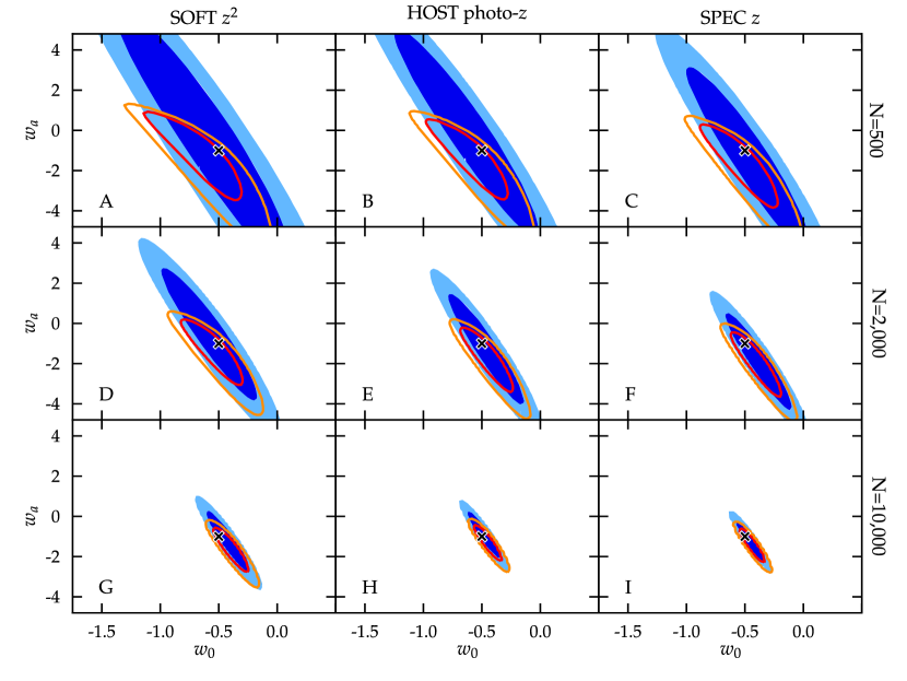
Figure 6: Likelihood contours in ($w_{0}$,$w_{a}$) space for the dark energy “Bootstrap Monte Carlo” simulations, based on data from SDSS and SNLS. Filled contours (in blue) show the 95% and 99.9% confidence boundaries from the SN data alone. Unfilled contours (in red and orange) show the combined constraint from SN, CMB, and BAO observations. A cross in each panel marks the location of the input cosmological parameters $w_{0}=-0.5$ and $w_{a}=-1.0$, which were used to generate the simulated observations. Each row (ABC, DEF and GHI) shows a set of simulations with 500, 2000, and 10000 SNe, respectively. The columns show results from using three different sources for the redshift priors. The first column (ADG) uses only the very weak $z^{2}$ prior. In the second column (BEH) we assume every simulated SN has a photometric redshift estimate from its host galaxy, and in the third column (CFI) we apply a strong spectroscopic prior.

The new up-and-coming surveys such as PS1, the Palomar Transient Factory, and Skymapper are best represented by simulations D and E, for which the FoM is improved by about a factor of 2. Not an insignificant gain, to be sure, but one that could easily be washed out by systematic uncertainties if they are not carefully controlled. The next leap forward, to be realized in the next decade by Pan-STARRS 4, JDEM and LSST, will bring the SN sample size to 10,000 or more objects, as in simulations G and H.

Using the DETF FoM as our principal barometer, our simulations suggest that a spectroscopy-free analysis using SOFT should be sufficient to capitalize on the very large SN samples coming in the next decade. With each new generation of SN surveys the sample size increases by a factor of 4–5, and the SOFT-based FoM increases by a factor of 2–3. A close look at the uncertainties on $w_{0}$ and $w_{a}$ in Table 3 highlights the fact that systematic effects will quickly become a dominant source of uncertainty. For a sample size of 2,000 objects the statistical uncertainty on $w_{0}$ from our Monte Carlo simulations is around $\pm 0.2$, which is already comparable to the expected level of systematic uncertainty.

How can these results inform our strategic choices for new and upcoming SN cosmology projects? We would argue that the new surveys can be successful relying on light-curve-based redshifts derived by SOFT or similar programs, informed by host galaxy photo-$z$’s when possible. For spectroscopic follow-up, instead of targeting the most likely TN SNe, cosmological analyses will be better served by focusing resources on objects that are given an ambiguous classification grade by SOFT. Most of these objects will be SNe of type Ib/c or Ia, perhaps with unusual colors or anomalous luminosities that make them difficult to classify. To the extent that spectroscopic measurements are able to provide a more definitive classification, we can sharpen SOFT’s ability to discriminate such marginal cases and help to reduce systematic errors from misclassifications.

In spite of the close connection to real data, the results of our bootstrap Monte Carlo approach are likely to be overly optimistic. We are necessarily overlooking the effects of sample selection and SN classification, and we have knowingly omitted systematic uncertainties from our analysis. In order to realize these optimistic predictions, it will be necessary to make adjustments and improvements to the SOFT program itself that will improve its precision and reduce systematic effects. In the following section we provide an outline for that future development.

5 Bias Corrections

As discussed in Section 2, our use of fixed shape light curve templates introduces an inherent bias into the parameter estimates that can be derived from each individual template. In this work we have addressed this problem by using the fuzzy intersection operator when combining membership functions. The fuzzy AND emphasizes collective agreement from all contributing templates, and therefore generally causes the individual biases to cancel out. In this section we consider two separate approaches that might reduce the effects of individual template biases by detecting and pre-emptively correcting for those location parameter offsets.

5.1 Template Calibration

Figure 7 illustrates how one could use a SN with a known location to measure the size and direction of template biases. The redshift and distance for our supposed calibration SN is marked by the “x.” After a SOFT comparison of our calibration SN against the model $M_{1}$ (based on SN 1999ee in Figure 7), we can measure the peak location of the $M_{1}$ cloud as $(z_{1},\mu_{e,1})$. Knowing the true location of the SN, we can then measure the distance from the cloud to the true position of the SN as $(\Delta z_{1},\Delta\mu_{e,1})$. This immediately gives us a bias correction vector $\beta_{1}=(-\Delta z_{1},-\Delta\mu_{e,1})$ that can be used to translate the entire probability cloud down to the true location of the peak. We can compute similar correction vectors for model $M_{2}$ (as shown in Figure 7) and all other models.

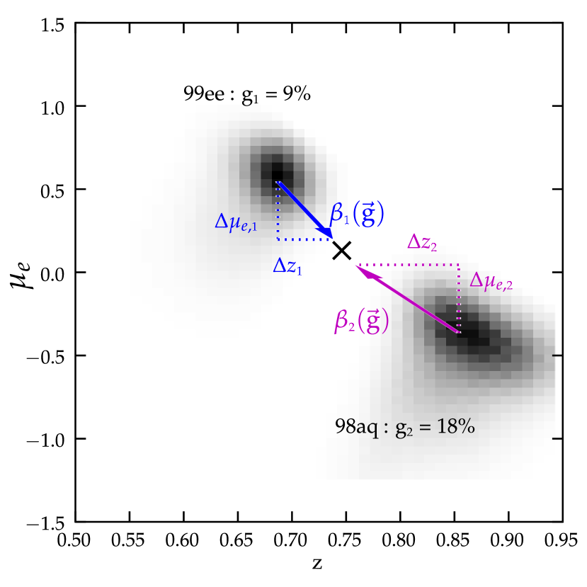
Figure 7: Illustration of the bias correction vectors $\beta_{j}$ that could be derived from a calibration of the SOFT template library. The background image shows the fuzzy membership functions for SNLS 04D2ja (as seen in Figure 1) from two separate template comparisons: SN 1999ee and 1998aq. The integrated membership grade $\gamma$ for each template is listed as a percentage. The goal of a template calibration process would be to derive a separate bias correction vector $\beta_{j}$ for each template. For any given candidate the size and direction of each template’s bias correction would be based on the unique pattern of integrated membership grades: ${\bf\Gamma}=\{\gamma_{1},\gamma_{2},\ldots\gamma_{N}\}$.

Unfortunately, once we derive a set of bias correction vectors using a particular calibration object, we can only apply them to other candidate SNe that are basically identical to the calibration object. If we have a candidate SN that is physically more similar to the model $M_{1}$ than our calibrator, then the $\beta_{1}$ vector shown in Figure 7 would be an over-correction. To avoid excessive bias correction, we need to scale the $\beta$ values separately for each candidate SN according to its similarity with the calibration object. For this purpose, we can use the set of all integrated membership function values from Eq. 5: ${\bf\Gamma}=\{\gamma_{1},\gamma_{2},\ldots\gamma_{N}\}$. As a first-order approximation, the bias correction function for model $M_{1}$ would be:

$$\beta_{1}(\bf\Gamma)=b_{11}\,\gamma_{1}+b_{12}\,\gamma_{2}+...+b_{1N}\,\gamma_{N}$$ (11)

Here we have introduced the parameters $b_{jk}$, which are two-dimensional constants that carry units of $z$ and $\mu_{e}$. If we have a candidate that is a 100% match to model $M_{1}$ then $\gamma_{1}=1$ and the $b_{11}$ parameter by itself would define the necessary bias correction. If instead the candidate has multiple non-zero $\gamma$ values for model $M_{1}$ would be a weighted sum of the $b_{jk}$ parameters.

Each template $M_{j}$ needs its own scalable bias correction function $\beta_{j}$. We can describe the complete set of bias correction functions for all N templates in matrix form:

$$\left[\begin{array}[]{c}\beta_{1}\\ \beta_{2}\\ \vdots\\ \beta_{N}\end{array}\right]=\left[\begin{array}[]{cccc}b_{11}&b_{12}&\cdots&b_{1N}\\ b_{21}&b_{22}&\cdots&b_{2N}\\ \vdots\\ b_{N1}&b_{N2}&\cdots&b_{NN}\\ \end{array}\right]\cdot\left[\begin{array}[]{c}\gamma_{1}\\ \gamma_{2}\\ \vdots\\ \gamma_{N}\\ \end{array}\right]$$ (12)

From this setup we can determine the appropriate values for the $b_{jk}$ parameters using a large calibration set of SNe with good light curves and spectroscopic redshifts. For each calibration SN, we would build up the single-template membership functions, and integrate them using Eq. 5. We would then measure the distance from the $g(z,\mu_{e}|M_{j})$ peak to the SN’s true location in order to get a $\beta_{j}$ value for each template. Every individual calibration SN thus provides an estimate for all components of the $\beta$ and ${\bf\Gamma}$ vectors. If the set of calibration SNe contains at least as many SNe as the template library, then the system of N equations in Equation 12 can be solved for the optimal set of $b_{jk}$ values. One possible source for calibration SNe would be to use a low-redshift Hubble flow training set (e.g. Jha et al., 1999) comprised of SNe that are far enough away to have small peculiar velocity errors ($cz\gtrsim 2500\,km\,s^{-1}$) but near enough that non-linear cosmological effects are negligible ($cz\lesssim 30,000\,km\,s^{-1}$).

This proposal is very simplistic, and may in fact be insufficient to account for the complexities of a real bias function. It is quite possible that the biases from individual templates are too inconsistent to allow for such a simple linear decomposition. One would need to see whether a consistent solution of Eq. 12 is possible, and whether the application of a bias correction vector is actually able to improve the results for a verification data set, such as the SDSS and SNLS SNe used here.

5.2 Peer to Peer Cosmology

An alternative method for removing location parameter biases is to use an approach that is based on selective comparisons. The SOFT method is founded on the assumption that two objects with very similar physical parameters ${\bf\Phi}$ will necessarily have very similar light curve shapes. The biases that we are trying to remove arise primarily due to light curve shape mismatches between the template and the candidate SN. Thus, if we could identify a group of SNe that have very similar ${\bf\Phi}$ values, then we would expect a direct comparison between group members to be largely free of bias.

One possibility would be to select candidate SNe that have very close matches in the template library. For example, we could pick out only those candidate objects that have a very strong match with a single template by elevating our template selection threshold to $\gamma>90\%$ or $95\%$. However, with only a few dozen templates in the library most SN candidates will not have a 90% match with any template, so the available sample size would be severely reduced.

A modification of this approach could overcome the limitations of a sparse template library by leveraging the very large SN data sets to come from future surveys. Suppose that a candidate SN X is observed at an unknown location $\theta$_X and we compare it against our N templates to get a vector of integrated membership grades ${\bf\Gamma_{X}}=(\gamma_{X1},\gamma_{X2},\ldots\gamma_{XN})$. A second candidate SN Y exists at a different location $\theta$_Y and has a different set of membership grades ${\bf\Gamma}_{Y}$. If these two objects have very similar physical characteristics, ${\bf\Phi}_{X}\approx{\bf\Phi}_{Y}$, then we should expect that the same templates that are good matches for SN X will also be similar to SN Y, so that ${\bf\Gamma}_{X}\approx{\bf\Gamma}_{Y}$.

This provides a straightforward means for collecting a group of similar SNe, which we will call a “peer group.” We compare all the available candidates against the template models, and then group together candidates that have a very similar pattern of membership grades ${\bf\Gamma}$. The members of this peer group generally will not have a perfect match in the template library, so no single template can provide an unbiased estimate for any of the group members. However, we do expect that any member of this peer group could provide an unbiased estimate for the location parameters of any other member in the group. All that is needed is to redefine the candidate SN members to take the place of the template library.

Recognizing that absolute distances are not necessary for cosmology, let us reduce the location vectors for our two peer SNe X and Y down to a pair of three-dimensional sub-vectors $\mbox{\boldmath$\vartheta$}_{X}=(z_{X},A_{V,X},t_{pk,X})$ and $\mbox{\boldmath$\vartheta$}_{Y}=(z_{Y},A_{V,Y},t_{pk,Y})$. The procedure for executing a peer to peer comparison is as follows:

1. Fit a smooth spline curve to the photometric data of SN X, allowing us to interpolate to any point in time.

2. Make a guess for $\mbox{\boldmath$\vartheta$}_{X}=(z_{X},A_{V,X},t_{pk,X})$

3. For every spectrum in the SOFT spectral library (Paper I, §2.2), apply the $z_{X}$ redshift, add reddening according to $A_{V,X}$, and shift in time to match $t_{pk,X}$.

4. Iteratively warp the adjusted spectra to force agreement with the observed $griz$ photometry of SN X.

5. Remove the effects of the assumed $\mbox{\boldmath$\vartheta$}_{X}$ from the warped spectra (i.e. apply a reverse time shift, dereddening, and a blue-shift) to get a rest-frame spectrophotometric model for SN X.

6. Repeat steps 1-5 for SN Y to get a rest-frame spectrophotometric model of SN Y under the assumption of a location $\mbox{\boldmath$\vartheta$}_{Y}=(z_{Y},A_{V,Y},t_{pk,Y})$.

At the end of this process we will have a pair of rest-frame spectrophotometric models $f_{X}(\lambda,t)$ and $f_{Y}(\lambda,t)$ giving the flux as a function of wavelength and time for both SN X and SN Y, at the assumed locations $\mbox{\boldmath$\vartheta$}_{X}$ and $\mbox{\boldmath$\vartheta$}_{Y}$. We now need to consider the relative luminosity distances for these two objects. Assuming that membership in the same peer group indicates that these two objects are physically almost identical, then they should have nearly the same intrinsic luminosity. This means that their relative luminosity distances $D_{L,X}$ and $D_{L,Y}$ are encoded in the flux ratio:

$$\mathcal{R}_{f}=\frac{f_{X}}{f_{Y}}=\left(\frac{D_{L,Y}}{D_{L,X}}\right)^{2}$$ (13)

With the addition of $\mathcal{R}_{f}$ we now have seven free parameters that define our rest-frame models for both objects. If the two SNe are in fact physically similar, and if we have guessed correctly about $\mbox{\boldmath$\vartheta$}_{X}$, $\mbox{\boldmath$\vartheta$}_{Y}$ and $\mathcal{R}_{f}$, then we should expect to see the same flux values as a function of wavelength and time: $f_{X}(\lambda,t)=\mathcal{R}_{f}\cdot f_{Y}(\lambda,t)$. This means that we can compute a posterior likelihood for each set of model parameters in the same manner that was used for Eq. 1:

$$\begin{array}[]{rl}p({\bf D}|&\mbox{\boldmath$\vartheta$}_{X},\mbox{\boldmath$\vartheta$}_{Y},\mathcal{R}_{f})=\prod\limits_{i=1}^{N}\frac{1}{\sqrt{2\pi}\sigma_{i}}\times\\ &\mbox{exp}\left(\frac{-(f_{X}(t_{i},\lambda_{i})-\mathcal{R}_{f}\cdot f_{Y}(t_{i},\lambda_{i}))^{2}}{2\sigma_{i}^{2}}\right)\end{array}$$ (14)

Here we are computing a flux difference $f_{X}-R_{f}f_{Y}$ at N points in time and wavelength. The flux uncertainty term, $\sigma_{i}$ could be computed as a quadratic sum of uncertainties from the SN X and SN Y models, accounting for the true observational errors for both SNe as well as additional error introduced by the spline fitting and spectral warping steps described above.

The posterior probability of Eq. 14 can now be treated in the same manner as the probabilities derived for the template-based SOFT comparisons in Section 2. After setting priors for all the components of $\mbox{\boldmath$\vartheta$}_{X}$, $\mbox{\boldmath$\vartheta$}_{Y}$ and $\mathcal{R}_{f}$, we can apply Bayes’ theorem as in Eq. 2. The resulting probability distribution can be marginalized over nuisance parameters to get a three-dimensional function in ($z_{X}$,$z_{Y}$,$\mathcal{R}_{f}$) space, which provides a direct constraint on any cosmological model.

There are several advantages to be gained by adopting this type of strategy for measuring cosmological parameters without spectroscopy. In addition to the bias minimization benefit, using peer to peer comparisons could provide a more robust model for the rest-frame ultraviolet light. For example, the rest-frame U band light from a SN at redshift z$>$0.2 will be observed in visual bandpasses (V or g). Thus, the g-band light curve of a z=0.2 template drawn from the Pan-STARRS survey is sufficient for comparison to the r-band light curve of a z=0.5 SN from the same survey. This approach also provides a natural set of internal consistency checks. As SN surveys begin to collect thousands of TN SN light curves, it may be possible to define peer groups with 10 or 20 members that all have very strongly similar light curve shapes. Each direct comparison between two objects in a peer group will provide an estimate of the redshifts for both objects. The consistency of redshift estimates for each object in the group provides a useful verification that the peer group is indeed defining a homogeneous set.

5.3 Spectral Library Bias

In addition to the biases of a sparse template library discussed above, SOFT may also suffer from systematic biases introduced by the spectral library. We have used the spectral templates of Hsiao et al. (2007) for normal Type Ia SNe, and those of Nugent et al. (2002) to describe overluminous 91T-like SNe and underluminous 91bg-like SNe. It has been suggested that the spectral properties of TN SNe may evolve with redshift (Blondin et al., 2006; Bronder et al., 2008; Foley et al., 2008a; Sullivan et al., 2009), in which case the use of these spectral templates based primarily on low-z SNe becomes inappropriate. This problem is particularly acute in the ultraviolet, where there can be substantial spectral variation (Ellis et al., 2008), and where it is especially difficult to collect a local sample (Foley et al., 2008b). The SALT2 light curve fitter addresses the UV problem by incorporating high redshift spectra to define the rest-frame UV (Guy et al., 2007). Extending the SOFT spectral library to avoid possible bias will be especially important when SOFT is applied for parameter estimation of TN SNe with z$>0.8$, where the rest-frame UV dominates the visible bandpasses.

6 Summary

In Paper I we introduced the SOFT program, using a set of fixed-shape light curve templates and the framework of fuzzy set theory for combining results from multiple templates. We applied SOFT as a SN classification tool in Paper I, and in this companion paper we have shown how SOFT can also be used to estimate parameters of cosmological interest: redshift $z$ and luminosity distance $\mu_{e}$. The SOFT method is distinct from light curve fitters such as MLCS and SALT in that it does not describe the light curve shape with a parameterized model. Given this fundamental distinction, SOFT may provide a valuable addition to the parametric fitters in that it could have smaller $-$ or at least different $-$ systematic uncertainties.

Using Type Ia SN light curves from the SDSS and SNLS data sets, we have performed a set of verification tests to demonstrate the accuracy of SOFT. We found that the SOFT redshift estimates are comparable to optical photo-z measurements for SDSS galaxies: both methods yield $\delta z=z_{SOFT}-z_{spec}$ residuals with an RMS scatter of approximately 0.05. Applying SOFT to derive (z,$\mu_{e}$) coordinate pairs for a joint SDSS$+$SNLS sample, we find an RMS scatter around the $\Lambda$CDM model of 0.18 mags in $\mu_{e}$ when including spectroscopic redshift priors. When SOFT analyzes the SDSS$+$SNLS sample with no spectroscopic information at all, we find the RMS scatter of Hubble residuals increases to 0.37 mags.

To investigate the near future of SN cosmology, we considered the degree to which a variable DE model can be constrained by larger SN samples containing thousands of light curves but very little spectroscopic follow-up. Using a bootstrap Monte Carlo approach, we simulated the distance and redshift estimates that might be obtained by SOFT for 9 different survey structures. We find that SOFT should be able to improve the DETF FoM by a factor of 2–3 with each new generation of SN surveys.

The SOFT program has not yet realized the full potential of its fuzzy logic approach, but we have outlined several pathways for improving the method and limiting systematic biases. We have proposed a straightforward method for using a training set to calibrate the template library, and have also presented a “Peer to Peer Cosmology” approach in which SOFT can identify groups of similar SNe and do a direct comparison to determine their redshifts and relative distances. This latter method may be especially applicable in upcoming SN surveys such as Pan-STARRS and LSST, which will have an abundance of well-sampled multi-color light curves, but comparatively little spectroscopic followup.

Acknowledgments: We would like to thank the anonymous referee for a thorough and critical reading of this work, which led to substantial improvements.

References

- Albrecht et al. (2006) Albrecht, A., et al. 2006, arXiv:astro-ph/0609591
- Aldering et al. (2006) Aldering, G., et al. 2006, ApJ, 650, 510
- Arnett (1982) Arnett, W. D. 1982, ApJ, 253, 785
- Astier et al. (2006) Astier, P., et al. 2006, A&A, 447, 31
- Barris & Tonry (2004) Barris, B. J., & Tonry, J. L. 2004, ApJ, 613, L21
- Blondin et al. (2006) Blondin, S., et al. 2006, AJ, 131, 1648
- Bronder et al. (2008) Bronder, T. J., et al. 2008, A&A, 477, 717
- Chevallier & Polarski (2001) Chevallier, M., & Polarski, D. 2001, International Journal of Modern Physics D, 10, 213
- Commins (2004) Commins, E. D. 2004, New Astronomy Review, 48, 567
- Davis et al. (2007) Davis, T. M., et al. 2007, ApJ, 666, 716
- Dombi (1982) Dombi, J. 1982, Fuzzy Sets and Systems, 8, 149
- Ellis et al. (2008) Ellis, R. S., et al. 2008, ApJ, 674, 51
- Foley et al. (2008a) Foley, R. J., et al. 2008a, ApJ, 684, 68
- Foley et al. (2008b) Foley, R. J., Filippenko, A. V., & Jha, S. W. 2008b, ApJ, 686, 117
- Gong et al. (2010) Gong, Y., Cooray, A., & Chen, X. 2010, ApJ, 709, 1420
- Guy et al. (2007) Guy, J., et al. 2007, A&A, 466, 11
- Guy et al. (2005) Guy, J., Astier, P., Nobili, S., Regnault, N., & Pain, R. 2005, A&A, 443, 781
- Hatano et al. (1998) Hatano, K., Branch, D., & Deaton, J. 1998, ApJ, 502, 177
- Hoeting et al. (1999) Hoeting, J. A., Madigan, D., Raftery, A. E., & Volinsky, C. T. 1999, Statistical Science, 14, 382
- Holtzman et al. (2008) Holtzman, J. A., et al. 2008, AJ, 136, 2306
- Hsiao et al. (2007) Hsiao, E. Y., Conley, A., Howell, D. A., Sullivan, M., Pritchet, C. J., Carlberg, R. G., Nugent, P. E., & Phillips, M. M. 2007, ApJ, 663, 1187
- Jha (2002) Jha, S. 2002, PhD thesis, Harvard University
- Jha et al. (1999) Jha, S., et al. 1999, ApJS, 125, 73
- Johnson & Crotts (2006) Johnson, B. D., & Crotts, A. P. S. 2006, AJ, 132, 756
- Kaiser et al. (2002) Kaiser, N., et al. 2002, in SPIE Conference Series, ed. J. A. Tyson & S. Wolff, Vol. 4836, 154–164
- Kessler et al. (2009) Kessler, R., et al. 2009, ApJS, 185, 32
- Kim & Miquel (2007) Kim, A. G., & Miquel, R. 2007, Astroparticle Physics, 28, 448
- Komatsu et al. (2009) Komatsu, E., et al. 2009, ApJS, 180, 330
- Komatsu et al. (2010) —. 2010, arXiv:1001.4538
- Kuznetsova & Connolly (2007) Kuznetsova, N. V., & Connolly, B. M. 2007, ApJ, 659, 530
- Law et al. (2009) Law, N. M., et al. 2009, PASP, 121, 1395
- Linder (2003) Linder, E. V. 2003, Physical Review Letters, 90, 091301
- Nugent et al. (2002) Nugent, P., Kim, A., & Perlmutter, S. 2002, PASP, 114, 803
- Oyaizu et al. (2008) Oyaizu, H., Lima, M., Cunha, C. E., Lin, H., Frieman, J., & Sheldon, E. S. 2008, ApJ, 674, 768
- Percival et al. (2010) Percival, W. J., et al. 2010, MNRAS, 401, 2148
- Poznanski et al. (2007) Poznanski, D., Maoz, D., & Gal-Yam, A. 2007, AJ, 134, 1285
- Rau et al. (2009) Rau, A., et al. 2009, PASP, 121, 1334
- Riello & Patat (2005) Riello, M., & Patat, F. 2005, MNRAS, 362, 671
- Riess et al. (1996) Riess, A. G., Press, W. H., & Kirshner, R. P. 1996, ApJ, 473
- Rodney & Tonry (2009) Rodney, S. A., & Tonry, J. L. 2009, ApJ, 707, 1064
- Sollerman et al. (2009) Sollerman, J., et al. 2009, ApJ, 703, 1374
- Sullivan et al. (2009) Sullivan, M., Ellis, R. S., Howell, D. A., Riess, A., Nugent, P. E., & Gal-Yam, A. 2009, ApJ, 693, L76
- Sullivan et al. (2006) Sullivan, M., et al. 2006, AJ, 131, 960
- Wood-Vasey et al. (2007) Wood-Vasey, W. M., et al. 2007, ApJ, 666, 694
- Zadeh (1965) Zadeh, L. A. 1965, Information and Control, 8, 338