Multi-site Observations of Pulsation in the Accreting White Dwarf SDSS J161033.64-010223.3 (V386 Ser)
Abstract
Nonradial pulsations in the primary white dwarfs of cataclysmic variables can now potentially allow us to explore the stellar interior of these accretors using stellar seismology. In this context, we conducted a multi-site campaign on the accreting pulsator SDSS J161033.64-010223.3 (V386 Ser) using seven observatories located around the world in May 2007 over a duration of 11 days. We report the best fit periodicities here, which were also previously observed in 2004, suggesting their underlying stability. Although we did not uncover a sufficient number of independent pulsation modes for a unique seismological fit, our campaign revealed that the dominant pulsation mode at 609 s is an evenly spaced triplet. The even nature of the triplet is suggestive of rotational splitting, implying an enigmatic rotation period of about 4.8 days. There are two viable alternatives assuming the triplet is real: either the period of 4.8 days is representative of the rotation period of the entire star with implications for the angular momentum evolution of these systems, or it is perhaps an indication of differential rotation with a fast rotating exterior and slow rotation deeper in the star. Investigating the possibility that a changing period could mimic a triplet suggests that this scenario is improbable, but not impossible.
Using time-series spectra acquired in May 2009, we determine the orbital period of SDSS J161033.64-010223.3 to be 83.8 2.9 min. Three of the observed photometric frequencies from our May 2007 campaign appear to be linear combinations of the 609 s pulsation mode with the first harmonic of the orbital period at 41.5 min. This is the first discovery of a linear combination between nonradial pulsation and orbital motion for a variable white dwarf.
1 Introduction to accreting white dwarf pulsators
Cataclysmic variables are interacting binary systems in which a late-type star loses mass to an accreting white dwarf. Photometric variations consistent with nonradial g-mode pulsations were first discovered in the cataclysmic variable GW Librae in 1998 (Warner & van Zyl, 1998; van Zyl et al., 2000, 2004); such pulsations had previously been observed only among the non-interacting white dwarf stars. This discovery has opened a new venue of opportunity to learn about the stellar parameters of accreting variable white dwarfs using asteroseismic techniques (e.g. Townsley et al., 2004). A unique model fit to the observed periods of the variable white dwarf can reveal information about the stellar mass, core composition, age, rotation rate, magnetic field strength, and distance (see the review papers Winget, 1998; Winget & Kepler, 2008; Fontaine & Brassard, 2008).
There are now thirteen accreting pulsating white dwarfs known (see van Zyl et al., 2004; Woudt & Warner, 2004; Warner & Woudt, 2004; Patterson et al., 2005a, b; Vanlandingham et al., 2005; Araujo-Betancor et al., 2005; Gänsicke et al., 2006; Nilsson et al., 2006; Mukadam et al., 2007b; Pavlenko, 2008; Patterson et al., 2008). Szkody et al. (2002a, 2007, 2010) are pioneering the effort to empirically establish the pulsational instability strip for accretors and to test the theoretical framework laid down by Arras et al. (2006). The instability strip(s) for these pulsators has to be established separately from the ZZ Ceti strip111Non-interacting hydrogen atmosphere (DA) white dwarfs are observed to pulsate in a narrow instability strip located within the temperature range 10800–12300 K for (Bergeron et al., 1995, 2004; Koester & Allard, 2000; Koester & Holberg, 2001; Mukadam et al., 2004; Gianninas et al., 2005), and are also known as the ZZ Ceti stars. because accretion enriches their envelopes with He and metals. This is distinct from the pure H envelope of the non-interacting DA white dwarfs, where H ionization causes them to pulsate as ZZ Ceti stars. Arras et al. (2006) find a H/HeI instability strip for accreting model white dwarfs with a blue edge near 12000 K for a 0.6 star, similar to the ZZ Ceti instability strip. They also find an additional hotter instability strip at 15000 K due to HeII ionization for accreting model white dwarfs with a high He abundance ( 0.38).
The spectrum of an accreting pulsator includes prominent broad absorption lines from the white dwarf as well as the central emission features from the accretion disk. When the orbital period of a cataclysmic variable is 80-90 min, it is near the evolutionary orbital period minimum, where the rate of mass transfer is theoretically expected to be the smallest /yr (Kolb & Baraffe, 1999). Due to the low rates of mass transfer, the white dwarf is expected to be the source of 90% of the optical light observed from these systems (Townsley & Bildsten, 2002). This makes it possible to detect white dwarf pulsations in these cataclysmic variables.
Accreting pulsators have probably undergone a few billion years of accretion and thousands of thermonuclear runaways. Studying these systems will allow us to address the following questions: to what extent does accretion affect the white dwarf mass, temperature, and composition and how efficiently is angular momentum transferred to the core of the white dwarf. These systems are also crucial in understanding the above effects of accretion on pulsations.
Asteroseismology can allow us to obtain meaningful mass constraints for the pulsating primary white dwarfs of cataclysmic variables. Previously any such constraints on the mass of the accreting white dwarf could only be established for eclipsing cataclysmic variables (e.g. Wood et al., 1989; Silber et al., 1994; Sing et al., 2007; Littlefair et al., 2008). Constraining the population, mass distribution, and evolution of accreting white dwarfs is also important for studying supernovae Type Ia systematics. For example, Williams et al. (2009) show empirically that the maximum mass of white dwarf progenitors has to be at least 7.1 thus constraining the lower mass limit for supernovae progenitors.
2 Motivation
Szkody et al. (2002b) deduced that SDSS J161033.64-010223.3 (V386 Ser; hereafter SDSS1610-0102) is a cataclysmic variable from early SDSS spectroscopic observations (Stoughton et al., 2002; Abazajian et al., 2003); SDSS has single-handedly led to a substantial increase in the number of known cataclysmic variables. Subsequently Woudt & Warner (2004) discovered photometric variations in the light curve of SDSS1610-0102 consistent with non-radial pulsations. They determined two independent pulsation modes with periods near 607 s and 345 s, also finding their harmonics and linear combinations in the data. Noting the amplitude modulation in the light curves, Woudt & Warner (2004) concluded that the dominant mode was a multiplet, but were unable to resolve it. They also determined the orbital period of 80.52 min from the observed double-humped modulation in their light curves.
We chose to target SDSS1610-0102 for a multi-site asteroseismic campaign from eleven possibilities known then for the following reasons. Previous observations of the system had revealed two independent pulsation frequencies, while several similar systems show no more than one pulsation frequency. Each independent pulsation frequency serves as a constraint on the stellar structure; detecting a larger number of frequencies is essential in obtaining a unique seismological fit. SDSS1610-0102 has an equatorial declination, making it easily accessible to observatories in both northern and southern hemispheres. The objective of the multi-site participation is to keep the sun from rising on the target star (Nather et al., 1990); reducing the gaps in the stellar data due to daytime increases the contrast between the true frequency and its aliases, thus making multi-site observations more effective than single-site observations.
3 Observations
We acquired optical time-series photometry on the accreting white dwarf pulsator SDSS1610-0102 over a duration of 11 days in May 2007 using multiple telescopes. Our multi-site campaign involved using the prime focus time-series photometer Argos (Nather & Mukadam, 2004) on the 2.1 m Otto Struve telescope at McDonald Observatory (MO), and the time-series photometer Agile (Mukadam et al., 2007a) on the 3.5 m telescope at Apache Point Observatory (APO). Both instruments are frame transfer CCD cameras devoid of mechanical shutters, where the end of an exposure and the beginning of a new exposure is triggered directly by the negative edges of GPS-synchronized pulses without any intervention from the data acquisition software. There is also no dead time between consecutive exposures from CCD read times, making Argos and Agile ideal instrumentation for the study of variable phenomena with millisecond timing accuracy. Argos and Agile consist of back-illuminated CCDs with an enhanced back-thinning process for higher blue quantum efficiency. Additionally, the E2V CCD 47-20 in Agile has an ultra-violet coating to enhance the wavelength efficiency of the region 200–370 nm to 35%. As Apache Point Observatory is located at an altitude of 2788 m, we expect to detect at least some of the blue photons in the range of 320–370 nm.
We utilized the Calar Alto Faint Object Spectrograph (CAFOS) in imaging mode on the 2.2 m telescope at Calar Alto Observatory (CAO) during the campaign. The duration between the FITS time stamp and the actual opening of the shutter is expected to be a fraction of a second. Network Time Protocol (NTP) is used to discipline the data acquisition computer, and we expect that the uncertainty in timing for a CAFOS image is of the order of 0.5 s. The SITe CCD in CAFOS has a quantum efficiency greater than 80% in the wavelength range of 370–780 nm. Data was acquired on the robotic 2.0 m Faulkes Telescope North (FTN) at Haleakala, Hawaii, using the instrument HawkCam1; this telescope belongs to the Las Cumbres Observatory Global Telescope (LCOGT) network. The data acquisition computer for HawkCam1 is synchronized to a GPS time server. The delay between the UTSTART timestamp in the FITS images and the actual opening of the mechanical shutter is expected to be of the order of a few milliseconds. This instrument contains an E2V CCD42-40, which is thinned and back-illuminated for blue sensitivity.
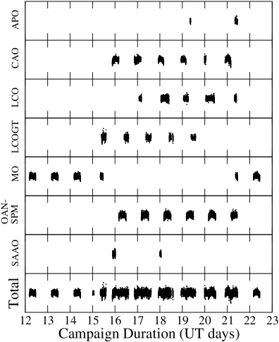
The camera SALTICAM (O’Donoghue et al., 2003) was used on the effective 10 m South African Large Telescope (SALT) at the South African Astronomical Observatory (SAAO) to acquire data for our campaign. The frame transfer time for this large format 2K 4K CCD is 0.1 s; the uncertainty in timing should be significantly smaller than a tenth of a second. The CCDs used in SALTICAM are thinned, back-illuminated, and made from deep depletion silicon which provides less fringing and additional sensitivity in the near infrared without photon loss in the blue and ultra-violet. SALTICAM has an efficiency greater than 80% in the wavelength range of 320–940 nm. Including atmospheric extinction and reflectivity losses at the different mirrors, SALTICAM has an efficiency greater than 60% from 380 to 840 nm. We observed on the 1.5 m telescope of the Observatorio Astrónomico Nacional in San Pedro Martir (OAN-SPM) using the instrument Ruca (Zazueta et al., 2000). Ruca comprises of the detector SITE1 SI003 CCD with a quantum efficiency greater than 55% in the wavelength range 500–800 nm. On the 2.5 m Irénée du Pont telescope at Las Campanas Observatory (LCO), we used the Direct CCD Camera (CCD), which includes a 2K 2K Tek CCD with a quantum efficiency greater than 70% in the wavelength range of 400–700 nm. Table 1 gives the journal of observations, and Figure 1 shows the extent of our coverage during the campaign.
| Telescope | Instrument | Observers | Start Time | Ending Time | Number of | ExpTime | Filter |
|---|---|---|---|---|---|---|---|
| (UTC) | (UTC) | Images | (s) | ||||
| APO 3.5 m | Agile | ASM | 19 May 2007 08:17:03 | 08:55:33 | 77 | 30 | BG40 |
| APO 3.5 m | Agile | ASM | 21 May 2007 08:19:36.1 | 11:09:36.1 | 340 | 30 | BG40 |
| CAO 2.2 m | CAFOS | AA | 15 May 2007 00:05:49.0 | 01:29:47.5 | 56 | 75 | Roeser BV |
| CAO 2.2 m | CAFOS | AA | 15 May 2007 21:05:20.4 | 03:37:49.7 | 576 | 25 | none |
| CAO 2.2 m | CAFOS | AA | 16 May 2007 03:38:06.1 | 03:58:22.7 | 27 | 30 | none |
| CAO 2.2 m | CAFOS | AA | 16 May 2007 20:43:01.2 | 21:01:40.1 | 22 | 35 | none |
| CAO 2.2 m | CAFOS | AA | 16 May 2007 21:01:56.2 | 21:19:09.4 | 23 | 30 | none |
| CAO 2.2 m | CAFOS | AA | 16 May 2007 21:19:24.7 | 04:02:19.0 | 598 | 25 | none |
| CAO 2.2 m | CAFOS | AA | 17 May 2007 22:18:01.6 | 03:57:36.6 | 502 | 25 | none |
| CAO 2.2 m | CAFOS | AA | 18 May 2007 22:36:00.1 | 03:56:11.4 | 441 | 25 | none |
| CAO 2.2 m | CAFOS | AA | 19 May 2007 22:15:41.6 | 22:28:50.6 | 20 | 25 | none |
| CAO 2.2 m | CAFOS | AA | 19 May 2007 22:29:06.5 | 22:37:54.4 | 11 | 30 | none |
| CAO 2.2 m | CAFOS | AA | 19 May 2007 22:40:37.8 | 00:12:00.4 | 62 | 35 | none |
| CAO 2.2 m | CAFOS | AA | 20 May 2007 00:13:11.5 | 00:44:15.4 | 28 | 40 | none |
| CAO 2.2 m | CAFOS | AA | 20 May 2007 00:44:30.9 | 02:06:20.6 | 43 | 35 | none |
| CAO 2.2 m | CAFOS | AA | 20 May 2007 21:45:26.1 | 23:34:01.6 | 122 | 35 | none |
| CAO 2.2 m | CAFOS | AA | 20 May 2007 23:34:17.7 | 00:54:14.4 | 77 | 30 | none |
| CAO 2.2 m | CAFOS | AA | 21 May 2007 00:54:29.8 | 01:02:21.7 | 11 | 25 | none |
| CAO 2.2 m | CAFOS | AA | 21 May 2007 01:02:39.7 | 01:06:57.9 | 6 | 30 | none |
| CAO 2.2 m | CAFOS | AA | 21 May 2007 01:07:16.4 | 02:37:28.3 | 88 | 35 | none |
| CAO 2.2 m | CAFOS | AA | 21 May 2007 02:37:44.6 | 03:29:59.7 | 63 | 30 | none |
| CAO 2.2 m | CAFOS | AA | 21 May 2007 03:30:15.0 | 03:40:49.2 | 16 | 25 | none |
| CAO 2.2 m | CAFOS | AA | 21 May 2007 03:41:12.2 | 03:51:36.1 | 14 | 30 | none |
| LCO 2.5 m | CCD | MRS, AS | 17 May 2007 01:39:26.4 | 03:14:38.1 | 101 | 40ααThe true exposure times are uneven and in excess of the given table entries by 0.03–0.05 s. | V |
| LCO 2.5 m | CCD | MRS, AS | 17 May 2007 03:15:51.3 | 04:01:04.7 | 61 | 30ααThe true exposure times are uneven and in excess of the given table entries by 0.03–0.05 s. | V |
| LCO 2.5 m | CCD | MRS, AS | 17 May 2007 04:01:45.4 | 04:31:19.0 | 46 | 25ααThe true exposure times are uneven and in excess of the given table entries by 0.03–0.05 s. | V |
| LCO 2.5 m | CCD | MRS, AS | 17 May 2007 04:34:20.4 | 05:42:11.8 | 86 | 35ααThe true exposure times are uneven and in excess of the given table entries by 0.03–0.05 s. | V |
| LCO 2.5 m | CCD | MRS, AS | 17 May 2007 05:46:22.7 | 06:10:28.1 | 25 | 45ααThe true exposure times are uneven and in excess of the given table entries by 0.03–0.05 s. | V |
| LCO 2.5 m | CCD | MRS, AS | 18 May 2007 01:05:50.7 | 02:20:54.2 | 101 | 30ααThe true exposure times are uneven and in excess of the given table entries by 0.03–0.05 s. | V |
| LCO 2.5 m | CCD | MRS, AS | 18 May 2007 02:21:43.3 | 05:32:14.0 | 293 | 25ααThe true exposure times are uneven and in excess of the given table entries by 0.03–0.05 s. | V |
| LCO 2.5 m | CCD | MRS, AS | 18 May 2007 05:32:50.8 | 09:05:45.5 | 362 | 20ααThe true exposure times are uneven and in excess of the given table entries by 0.03–0.05 s. | V |
| LCO 2.5 m | CCD | MRS, AS | 18 May 2007 09:06:06.7 | 09:25:37.6 | 31 | 25ααThe true exposure times are uneven and in excess of the given table entries by 0.03–0.05 s. | V |
| LCO 2.5 m | CCD | MRS, AS | 18 May 2007 09:26:11.3 | 09:51:10.2 | 35 | 30ααThe true exposure times are uneven and in excess of the given table entries by 0.03–0.05 s. | V |
| LCO 2.5 m | CCD | MRS, AS | 19 May 2007 01:16:31.5 | 08:32:53.0 | 650 | 25ααThe true exposure times are uneven and in excess of the given table entries by 0.03–0.05 s. | V |
| LCO 2.5 m | CCD | MRS, AS | 20 May 2007 01:02:52.3 | 10:11:13.3 | 843 | 25ααThe true exposure times are uneven and in excess of the given table entries by 0.03–0.05 s. | V |
| LCO 2.5 m | CCD | MRS, AS | 21 May 2007 01:59:23.6 | 02:42:51.1 | 62 | 28ααThe true exposure times are uneven and in excess of the given table entries by 0.03–0.05 s. | V |
| LCO 2.5 m | CCD | MRS, AS | 21 May 2007 07:30:19.0 | 09:48:57.5 | 190 | 25ααThe true exposure times are uneven and in excess of the given table entries by 0.03–0.05 s. | V |
| LCOGT 2.0 m | HawkCam1 | Robotic | 15 May 2007 09:28:33.5 | 14:30:07.2 | 261 | 60 | V |
| LCOGT 2.0 m | HawkCam1 | Robotic | 16 May 2007 09:42:41.3 | 14:29:40.8 | 244 | 60 | V |
| LCOGT 2.0 m | HawkCam1 | Robotic | 17 May 2007 08:49:59.3 | 14:33:50.9 | 291 | 60 | V |
| LCOGT 2.0 m | HawkCam1 | Robotic | 18 May 2007 09:53:09.2 | 12:03:08.0 | 113 | 60 | V |
| LCOGT 2.0 m | HawkCam1 | Robotic | 18 May 2007 13:32:21.9 | 14:15:57.6 | 38 | 60 | V |
| LCOGT 2.0 m | HawkCam1 | Robotic | 19 May 2007 09:17:22.6 | 14:10:54.9 | 195 | 60 | V |
| MO 2.1 m | Argos | ASM, BF | 12 May 2007 04:29:30.0 | 11:17:10.0 | 1223 | 20 | BG40 |
| MO 2.1 m | Argos | ASM, BF | 13 May 2007 04:07:39.0 | 11:10:19.0 | 1268 | 20 | BG40 |
| MO 2.1 m | Argos | ASM, BF | 14 May 2007 04:12:44.0 | 11:19:04.0 | 1279 | 20 | BG40 |
| MO 2.1 m | Argos | ASM, BF | 15 May 2007 08:24:49.0 | 11:12:49.0 | 504 | 20 | BG40 |
| MO 2.1 m | Argos | ASM, BF | 21 May 2007 08:58:08.0 | 10:58:08.0 | 240 | 30 | BG40 |
| MO 2.1 m | Argos | ASM, BF | 22 May 2007 04:09:51.0 | 11:00:39.0 | 1218 | 20 | BG40 |
| OAN-SPM 1.5 m | Ruca | GT, SVZ | 16 May 2007 03:59:53 | 06:15:32 | 200 | 35 | BG40 |
| OAN-SPM 1.5 m | Ruca | GT, SVZ | 16 May 2007 06:17:15 | 11:48:51 | 581 | 25 | BG40 |
| OAN-SPM 1.5 m | Ruca | GT, SVZ | 17 May 2007 04:09:31 | 11:49:48 | 950 | 20 | BG40 |
| OAN-SPM 1.5 m | Ruca | GT, SVZ | 18 May 2007 04:12:23 | 11:47:23 | 799 | 25 | BG40 |
| OAN-SPM 1.5 m | Ruca | GT, SVZ | 19 May 2007 04:20:45 | 11:45:23 | 850 | 25 | BG40 |
| OAN-SPM 1.5 m | Ruca | GT, SVZ | 20 May 2007 03:56:09 | 11:40:19 | 892 | 25 | BG40 |
| OAN-SPM 1.5 m | Ruca | GT, SVZ | 21 May 2007 04:01:27 | 04:47:46 | 50 | 50 | BG40 |
| OAN-SPM 1.5 m | Ruca | GT, SVZ | 21 May 2007 04:50:12 | 10:39:22 | 500 | 35 | BG40 |
| SAAO 10 m | SALTICAM | RS | 15 May 2007 21:36:18.6 | 00:23:41.3 | 605 | 3 | B-S1ββThe B-S1 filter is nearly the same as a Johnson B filter. |
| SAAO 10 m | SALTICAM | RS | 17 May 2007 23:49:51.7 | 01:15:55.5 | 287 | 10 | B-S1ββThe B-S1 filter is nearly the same as a Johnson B filter. |
4 Data Reduction and Analysis
We used a standard IRAF reduction to extract sky-subtracted light curves from the CCD frames using weighted circular aperture photometry (O’Donoghue et al., 2000). After extracting the light curves, we divided the light curve of the target star with a sum of one or more comparison stars using brighter stars for the division whenever available as opposed to faint stars; this choice leads to comparatively lower noise in the target star light curve after the process of division. After this preliminary reduction, we brought the data to a fractional amplitude scale () and converted the mid-exposure times of the CCD images to Barycentric Coordinated Time (TCB; Standish, 1998). The first data point of the campaign was used to define a reference zero time of 2454232.693409 TCB, which we applied to all the reduced light curves. We then computed a Discrete Fourier Transform (DFT) for all the individual observing runs up to the Nyquist frequency.
All stellar pulsators reveal wavelength-dependent amplitudes whenever their atmospheres suffer from limb-darkening effects; this is also observed to be true for white dwarf pulsators (Robinson et al., 1995). Copperwheat et al. (2009) have measured the broadband amplitudes of the pulsation frequencies in SDSS1610-0102, confirming the trend of larger amplitudes at bluer wavelengths. Including photons redward of 6500 Å, which are less modulated by the pulsation process, reduces the measured amplitude by as much as 20–40% (Kanaan et al., 2000; Nather & Mukadam, 2004).
Based on the pulsation amplitude of the dominant mode, we divided the data from different sites, acquired using different instruments with distinct wavelength responses and different filters, into three groups. The data from the MO 2.1 m, APO 3.5 m, and the SAAO 10 m telescopes along with the Roeser BV data acquired on the 15th of May using the CAO 2.2 m telescope constitute Group 1; these data reveal an amplitude of 29.290.51 mma for the 609 s mode. The data obtained from the LCO 2.5 m, LCOGT 2.0 m, and OAN-SPM 1.5 m telescopes, that form Group 2, yield an amplitude of 25.520.59 mma. The Calar Alto white light data that forms Group 3 amounts to an amplitude of 22.31.1 mma. These values of amplitude are not consistent with each other within the uncertainties. The pulsation amplitude obtained for sites in Group 2 is approximately 15% lower compared to sites in Group 1, while Group 3 shows a pulsation amplitude 31% lower than Group 1. Hence to even out the 15–31% amplitude differences between the various data segments, we scaled the Group 2 data by a factor of 1.15 and Group 3 data by a factor of 1.31. Without scaling the data, we would effectively be fitting a constant amplitude sinusoid to a multi-site light curve with different embedded amplitudes. After this scaling, the entire 11-day long light curve could be subjected to least squares analysis.
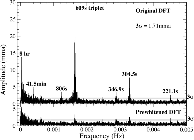
Blue bandpass filters are ideal to study these hot white dwarf variables. Typically we are forced to acquire white light data whenever the photon count rate proves to be inadequate. Scaling these noisy light curves to match the pulsation amplitude of the other higher S/N blue observations also implies scaling the noise with the same factor. The drawback of scaling the data is an overall increase in noise; we do find that the 3 level increases from 1.49 mma to 1.71 mma as a result of scaling. By comparison, the highest amplitude peak in the 609 s triplet increases from 26.10 mma to 28.78 mma due to scaling.
We do not have to worry about scaling the other observed frequencies similarly, except the 41.5 min period, as they are all low amplitude modes. Their amplitudes in the various data segments are already consistent with each other within the uncertainties. We also checked explicitly that the chosen scaling does not alter the results of the least squares analysis for any of the other frequencies, and no artificial frequencies or frequency splittings arise due to this scaling. Note that the amplitudes obtained for the 41.5 min period for sites in Group 1 and Group 2 are 5.220.50 mma and 3.920.58 mma respectively. Sites in Group 2 show an amplitude approximately 33% lower compared to sites in Group 1. The wavelength dependence of the 41.5 min period differs from the 609 s mode; this is consistent with the findings of Copperwheat et al. (2009). The Calar Alto white light data (Group 3) are too noisy to determine a reliable amplitude for the 41.5 min period. This implies that our chosen scaling of 1.15 improves the amplitude differences for the 41.5 min period as well, and evens it out to the point that the data segments have an amplitude consistent with each other within uncertainties.
All of the subsequent data analysis and the Discrete Fourier Transform (DFT) shown in Figure 2 is based on this scaled multi-site 11-day long light curve obtained during the campaign. Although we computed the DFT right up to the Nyquist frequency of 0.025 Hz, there were no significant peaks above the 3 limit of 1.71 mma222One milli modulation amplitude (mma) equals 0.1% amplitude in intensity, corresponding to a 0.2% peak-to-peak change; one mma is equal to 1.085 mmag. between 0.005 and 0.025 Hz. Hence the interesting portion of the DFT is shown in Figure 2. We determine the amount of white noise in the light curve empirically by using a shuffling technique (see Kepler, 1993). All the best-fit frequencies were initially subtracted to obtain a prewhitened light curve. Preserving the time column of this light curve, we shuffled the corresponding intensities. This exercise destroys any coherent signal in the light curve while keeping the time sampling intact, leaving behind a shuffled light curve of pure white noise. The average amplitude of a DFT computed for the shuffled light curve is close to the 1 limit of the white noise. After shuffling the light curve ten times, we average the corresponding values for white noise to determine a reliable 3 limit.
Table 2 indicates the best fit periodicities along with the least squares uncertainties we obtained using the program Period04 (Lenz & Breger, 2005). We cross-checked the periods, amplitudes, and phases obtained with our own linear and non-linear least squares code and find that the values obtained from both programs are almost identical. The program Period04 has the added advantage of computing Monte-Carlo uncertainties, which are shown as italicized numbers in Table 2. Previous papers on SDSS1610-0102 did not resolve the triplet (Woudt & Warner, 2004; Copperwheat et al., 2009), and hence their determinations of the dominant period differ slightly in value from ours (see the second to last paragraph in section 7). However the pulsation spectrum in 2007 is essentially similar to that observed in 2004 and 2005.
| Identification | Frequency (Hz) | Period (s) | Amplitude (mma) | PhaseααWe refer to the time of the first zero crossing of the sine curve as its phase, i.e. =0 for a sine curve sin() defined over the range from 0 to 2. The phases are defined with respect to a reference zero time of 2454232.693409 TCB. (s) |
|---|---|---|---|---|
| F609a | 1641.796 0.028 | 609.0893 0.010 | 28.78 0.50 | 596.0 2.2 |
| 0.024 | 0.0089 | 0.63 | 2.8 | |
| F609b | 1643.074 0.057 | 608.615 0.021 | 8.22 0.51 | 255.0 6.1 |
| 0.057 | 0.021 | 0.49 | 8.2 | |
| F609c | 1640.665 0.071 | 609.509 0.026 | 7.95 0.66 | 50.3 6.9 |
| 0.082 | 0.031 | 0.79 | 9.1 | |
| 2 F609 | 3283.939 0.040 | 304.5124 0.0037 | 7.46 0.40 | 132.0 2.7 |
| 0.053 | 0.0049 | 0.56 | 3.3 | |
| 2 F609 | 3282.534 0.073 | 304.6427 0.0068 | 4.03 0.40 | 139.9 5.0 |
| 0.089 | 0.0082 | 0.52 | 6.3 | |
| F806 | 1240.517 0.071 | 806.115 0.046 | 3.62 0.40 | 483 14 |
| 10 | 6.5 | 1.4 | 130 | |
| F221 | 4523.14 0.10 | 221.0854 0.0049 | 2.59 0.40 | 201.0 5.4 |
| 29 | 1.4 | 1.2 | 78 | |
| F347 | 2882.582 0.076 | 346.9112 0.0091 | 3.41 0.40 | 91.6 6.5 |
| 23 | 2.8 | 1.5 | 96 | |
| F41.5m | 401.310 0.053 | 2491.84 0.33 | 4.90 0.40 | 826 32 |
| 0.075 | 0.46 | 0.49 | 45 | |
| F8h | 34.766 0.015 | 28764 13 | 15.76 0.43 | 5860 110 |
| 0.023 | 19 | 0.56 | 130 |
Note that we also concatenated all the light curves from various sites without any scaling and computed the corresponding unscaled DFT, to find that it showed the same peaks as the DFT obtained after scaling the data. Additionally, we computed DFTs for the unscaled light curves from the first and second groups as defined earlier. These DFTs also revealed the same frequency set as shown in Figure 2. These tests show that scaling the data did not introduce any artificial new frequencies in our data set. In order to compute the best-fit periodicities for the unscaled light curve, we subjected it to Period04 similar to the procedure carried out for the scaled data. The best-fit values for the scaled and unscaled data are very similar, lending credence to the process of scaling the multi-site data, especially in its ability to preserve the original frequency set without introducing any new artifacts.
Although three of the seven sites boast millisecond timing accuracy, others like CAFOS involve a 0.5 s timing uncertainty per image. To test the effects of timing uncertainty on our results, we simulated a light curve including all ten frequencies listed in Table 2 along with their respective amplitudes, adding in white noise with an amplitude of 2 mma. Using the same time sampling as the real data, we added in a Gaussian uncertainty of = 2 s to each point to account for timing errors such as software delays in time-shared data acquisition computers, jitter in the opening of mechanical shutters, etc. This is worse than the worst case possible for badly synchronized clocks. Our results show that we are still able to recover the closely spaced frequencies of the 609 s triplet from the simulated light curve; the output best-fit period values were at most 0.003% different from the values used to generate the simulated light curve. Amplitudes and phases were affected at the 2% level or less. This result is not surprising given that the timing uncertainty is significantly smaller than the 609 s period, and the S/N ratio improves with each passing cycle.
5 Determining the orbital period
We acquired followup time-series spectroscopy on SDSS1610-0102 on the 28th of May, 2009, using the Dual Imaging Spectrograph (DIS) mounted on the APO 3.5 m telescope with intermediate resolution gratings (resolution about 2 Å) and a 1.5 arcsec slit. Our goal was not to get a precise determination of the orbital period, but to measure the orbital frequency well enough to identify it or any of its harmonics present in the campaign DFT. The spectroscopic data cover a period of just about 3 hours, adding up to a total of sixteen 10-min exposures. Individual exposures had a S/N of about 10 for the lines and 5–7 for the continuum. Standard IRAF routines were utilized for data reduction and subsequent flux and wavelength calibration. We used a boxcar smoothing over 3 points prior to implementing the centroid-finding routine in the IRAF splot package to obtain the equivalent widths and fluxes for the hydrogen Balmer lines. Fitting a sine curve to the radial velocity curves for each line, we determined the velocity of the center of mass , the semi-amplitude K, the orbital period , and the time of the red-to-blue crossing of the emission lines T0; these values are shown below in Table 3. Note that the exposure times constitute a non-negligible part of the orbital period; this causes some amplitude reduction. The amplitude values listed in Table 3 have been corrected for this effect. The top panel of Figure 3 shows the complete combined spectrum.
| Balmer | Velocity of the Center | Semi-amplitude | T0ααThe time of red-to-blue crossing of the emission lines T0 is given in minutes from 0 hr UTC on 28 May 2009. | Orbital Period |
|---|---|---|---|---|
| Line | of Mass (km/s) | K (km/s) | (min) | (min) |
| Hα | -23 2 | 96 14ββSince the exposure time was non-negligible compared to the orbital period, the amplitude values have been corrected to account for the resulting reduction effect. | 410 | 83 |
| Hβ | 28 3 | 208 23ββSince the exposure time was non-negligible compared to the orbital period, the amplitude values have been corrected to account for the resulting reduction effect. | 412 | 86 |
Emission lines from the accretion disk and the hot spot, where the matter stream hits the accretion disk, affect the spectral lines in cataclysmic variables. As a result, the velocity of the center of mass can be different for different Balmer lines, and may even have different signs (see Table 3). However the determination of the orbital period from both lines is consistent with each other within uncertainties.
We also applied the double Gaussian method outlined by Schneider & Young (1980) and developed by Shafter (1983) on the Hα line. This method involved the convolution of two Gaussian functions of opposite signs and equal FWHM of 300 km/s, chosen to be the same order as the wavelength resolution. A peak separation of 1800 km/s was used to reach further into the wings without compromising too much on the signal-to-noise ratio. This ensured that the measured radial velocities traced the inner part of the accretion disc, where azimuthally symmetric structure traces the orbital motion of the white dwarf. This technique produced the radial velocity curve (bottom panel of Figure 3) that led to an orbital period determination of 83.8 2.9 min. This spectroscopic determination is consistent with the photometric measurement of 83.061 0.011 min (obtained from 1/2 F41.5m) within the uncertainties. This orbital period not only indicates that SDSS1610-0102 is close to the period minimum, but also includes SDSS1610-0102 within the 80–86 min period-minimum spike that is largely made up of white dwarf dominated cataclysmic variables (Gänsicke et al., 2009).
Woudt & Warner (2004) observed a double-humped modulation in their light curves, and determined values of 87.5 1.8 min and 83.9 4.7 min for the orbital period. Using the first harmonic of the orbital period, they deduced additional measurements of 81.9 1.2 min and 81.2 0.4 min; these photometric determinations have lower uncertainties compared to the direct measurements above inspite of their lower amplitude because they involve twice the number of cycles compared to the orbital period itself. Large gaps in the combined light curve prevented Woudt & Warner (2004) from identifying a unique orbital period, and they present the alternatives of 80.52 min and 85.08 min. Computing a weighted average from their individual measurements above, weighted inversely as the uncertainties, we arrive at an orbital period determination of 83.7 1.4 min. This value is consistent with the orbital period measurement of 83.8 2.9 min from the Hα line.
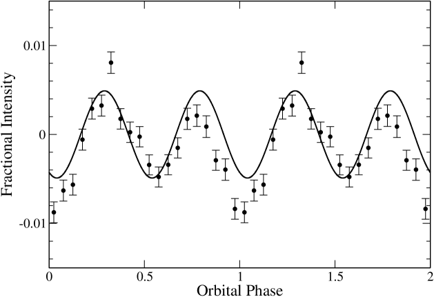
We pre-whitened all the frequencies from our 11-day light curve except for the 41.5 min periodicity, and folded it on the orbital period. The folded light curve and its running average are shown in Figure 4 to indicate its apparent double-humped nature. This pulse shape is different from the one shown by Woudt & Warner (2004), but it is consistent with the least squares analysis as expected. Table 2 reveals that apart from the first harmonic, no other period related to the orbital motion is observed. Hence we should expect to see two pulses with a period of about 41.5 min at an amplitude of 4.9 mma in the folded light curve. The pulse shape from Figure 4 fits a sine curve of period 41.24 min with an amplitude of 4.3 mma.
Several short period cataclysmic variables show similar double-humped light curves (Patterson et al., 1998; Rogoziecki & Schwarzenberg-Czerny, 2001; Dillon et al., 2008), and in some cases the orbital period has been independently determined using eclipses to confirm that the photometric and spectroscopic periods are actually the same within uncertainties. Robinson et al. (1978) proposed that a double humped variation is observed when the bright spot, where the accretion stream hits the white dwarf, is visible even when it is behind the optically thin disk. However Zharikov et al. (2008) and Aviles et al. (2010) argue that the permanent double-humped light curve is an attribute of bounced-backed systems; these systems consist of cataclysmic variables that have evolved beyond period minimum with quiescent accretion disk radii at a 2:1 resonance.
The accreting pulsating white dwarf constitutes a clock in orbit; the changing light travel time during an orbit is reflected in the pulse arrival times. The observed phase of the clock (O) compared to the phase of a stationary clock at the same period (C) should show a modulation at the orbital period (Winget et al., 2003; Mullally et al., 2008). We used the O-C method (with a small modification) to attempt a detection of the orbiting motion of the 609 s clock. However our uncertainties of 4–5 s were too large to reveal the expected sub-second change in light travel time during the orbiting motion of the white dwarf.
6 Identification of independent frequencies
Each independent pulsation frequency is a constraint on the structure of the star. Harmonics and linear combinations in our data merely arise as a result of non-linearities introduced by relatively thick convection zones (Brickhill, 1992; Brassard et al., 1995; Wu, 2001; Montgomery, 2005). Identifying the linearly independent frequencies in a pulsation spectrum is the first step to undertake in seismology.
Of the several periods shown in Figure 2, we suspect that the longest observed period of 28764 s or 8 hr is related to airmass or extinction variations or possibly the gaps in the 11-day light curve. Other cataclysmic variables have shown photometric or radial velocity periods that are much longer than the orbital period and bear no relation to it. For example, Woudt & Warner (2002) discuss long photometric periods such as the 2 hr modulation in GW Librae, a possible 3 hr period in FS Aur, and a 4.6 hr period in V2051 Oph. Tovmassian et al. (2007) show that the precession of the magnetically accreting white dwarf can successfully explain such long periods. However in this case, we do not believe that the 8 hr period is stellar in origin. The 2491.84 s or the 41.5 min period is clearly the first harmonic of the orbital period, measured spectroscopically to be 83.8 2.9 min. This identification is consistent with Woudt & Warner (2004).
The 609 s triplet is clearly an independent pulsation mode since it has the highest amplitude of all observed periods; typically harmonics and linear combinations have lower amplitudes than the parent modes. We can also readily identify the periods close to 304.5 s as the first harmonic of the 609 s triplet. A triplet can be expected at 304.5 s because the harmonic of a triplet should also be a triplet. However we are unable to resolve it, due most likely to the relatively lower amplitudes compared to the 609 s triplet.
There is also a small chance that the 609 s photometric period represents the rotation of the star, and we are misinterpreting it as nonradial pulsation. SDSS1610-0102 is neither strongly magnetic nor a source of x-rays, and therefore we do not expect to see a rotating hot spot as in the intermediate polars. It is difficult for a hot spot or belt to match the observed pulse shape of the 609 s period. If the 609 s period was the rotation period of the star, it would also be difficult to explain the evenly spaced triplet, but the triplet could perhaps have been caused by reprocessing or reflection effects. The ratio of the UV to optical pulsation amplitude of the 609 s period is consistent with low order g-mode pulsations (Szkody et al., 2007). For all of these reasons collectively, nonradial pulsation is certainly the favourable model to explain the 609 s photometric triplet. However please note that we are currently unable to absolutely exclude the possibility that the 609 s period is the rotation period of the star. For the rest of this paper, we will adopt the more likely model of nonradial pulsation for the 609 s triplet.
Let F41.5m, F806, F609, F347, and F221 denote the frequencies corresponding to the 41.5 min, 806 s, 609 s, 347 s, and 221 s periods. The linear combinations in our frequency set are: F221 = 3 F609 - F41.5m, F347 = 2 F609 - F41.5m, and F806 = F609 - F41.5m. Note that the amplitudes of all the proposed combination modes are smaller than the suggested parent modes as expected. Justifying the frequency F221 involves invoking 3 F609, which has not been observed directly. Woudt & Warner (2004) identify F347 as a second independent pulsation mode; however given the relation F347 = 2 F609 - F41.5m within uncertainties, we arrive at the inevitable conclusion that it is merely a linear combination mode.
This is probably the first instance for pulsating white dwarfs where linear combination frequencies have apparently emerged as a result of an interplay between a non-radial pulsation mode F609 and a harmonic of the orbital frequency F41.5m. The idea of a physical interaction between nonradial pulsation and tides caused by orbital motion may be relevant here. We defer a thorough investigation to a future theoretical paper.
7 Scrutinizing the pulsation triplet at 609 s
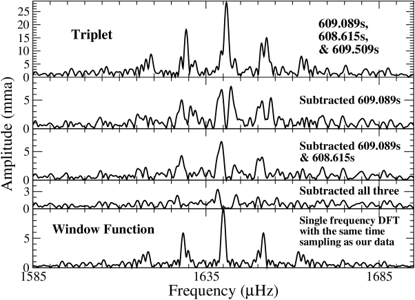
A measure of the gross ability of our data to resolve the components of the 609 s mode is evident from a comparison of the DFT and the window function, shown in the top and bottom panels of Figure 5 respectively. The window function is the DFT of a single frequency noiseless sinusoid sampled at exactly the same times as the actual light curve. Comparing the DFT to the window function unambiguously reveals the low frequency component and definite additional width, indicating the presence of more than one frequency. Using least squares analysis in conjunction with the technique of prewhitening, we are able to separate these resolved components. Prewhitening is the standard procedure for isolating and characterizing closely spaced spectral components; it involves subtracting out the best fit for the highest amplitude component of the multiplet from the light curve and re-computing the DFT. Carrying out this procedure for the 609.089 s period gives clear residuals with similar amplitude at similar spacing above and below in frequency, as shown in the second panel of Figure 5. Continuing to prewhiten with the 608.615 s (third panel) and then the 609.509 s periods (fourth panel) leads to marginal residual power near the 3 detection limit of 1.71 mma. This exercise demonstrates that the 609 s mode is made up of three components in the form of a triplet as listed in Table 2.
Measured pulsation amplitudes are typically lower than the intrinsic pulsation amplitudes due to geometric cancellation. This effect has three independent causes: disk averaging, inclination angle, and limb darkening. The inclination angle dictates the distribution of bright and dark zones in our view for a given mode; this introduces a large amount of scatter in observed pulsation amplitudes. Eigenmodes with different values exhibit different cancellation patterns (see Dziembowski 1977; Pesnell 1985). Hence we did not expect that all members of the 609 s triplet should have had the same amplitude.
Given that the implications of the triplet spacing are most unexpected, we conducted simulations to verify whether the triplet is indeed genuine or merely caused by a singular changing period. Although the pulsation period of a non-interacting ZZ Ceti only drifts due to stellar cooling (Kepler et al., 2000), the period of an accreting pulsator can drift on a faster timescale. During a dwarf nova outburst, an accreting white dwarf is heated to temperatures well beyond the instability strip and it ceases to pulsate (Szkody, 2008; Copperwheat et al., 2009; Szkody et al., 2010, e.g.). Once the white dwarf has cooled down close to its quiescent temperature and pulsations have resumed in the star, Townsley et al. (2004) explain how mode frequencies can drift a little due to the continued cooling of the outer envelope. They calculate that the longer period modes such as the 609 s mode should drift at the rate of d/dt - Hz/s. This expected model drift rate from the cooling of the outer envelope is much faster than the observed drift rate of d/dt - Hz/s for ZZ Ceti pulsators from the cooling of the entire star (Kepler et al., 2005; Mukadam et al., 2003, 2009). During our 11 day campaign, we should expect a drift in the pulsation period of the order of 1 Hz, comparable to the observed triplet spacing. Hence it becomes necessary to check whether a drifting period is responsible for the observed triplet, a fairly general way of introducing spurious peaks in the DFT.
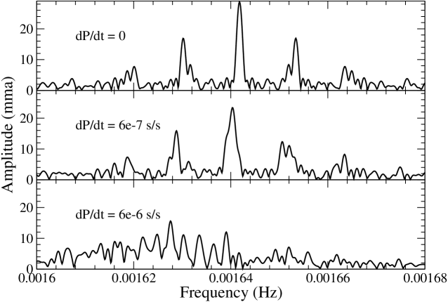
As a first step, we simulated constant-amplitude light curves with a single variable period near 609 s; the period was varied at different non-zero constant rates. The goal of the simulation was to check if it is possible to fit a triplet to any of the generated light curves, while processing them in the same manner as the real light curve from the campaign. For each drift rate dP/dt, we simulated a light curve with exactly the same time sampling as the real data, adding in Gaussian noise with an amplitude comparable to the observed white noise. We computed a DFT from the simulated light curve, and then used the techniques of least squares analysis and prewhitening to determine its frequency components, proceeding in exactly the same way as the real data.
Figure 6 shows the DFTs corresponding to the drift rates dP/dt =6 s/s and dP/dt =6 s/s, also including the DFT of a single constant period at 609 s for reference. Figure 6 clearly demonstrates that the amplitude of the DFT based on the 11-day simulated light curve is inversely proportional to the drift rate; faster the drift rate of the period, smaller the amplitude of the variable period in the DFT. The drift rate of the period has to be fast enough to cause a triplet spacing of 1.2 Hz in 11 days, and slow enough that the amplitude of the DFT does not fall significantly below the simulation amplitude. We find that the drift rate of 6 s/s comes close to reproducing the triplet spacing. However we are unable to use non-linear least squares code to fit three closely-spaced frequency components to the light curve simultaneously, indicating that they are not resolved.
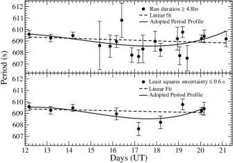
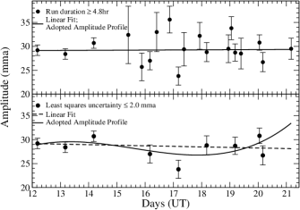
For the second step, we simulated mono-periodic signals whose period and amplitude vary continuously as low order functions. In order to keep our simulations realistic, we determined possible low-order functions using the observed data. To this end, we identified 19 runs of 4.8 hr duration or longer, acquired during the course of the campaign. Figure 7 indicates our measurements of period and amplitude for these runs; the amplitudes from filterless data are scaled by a factor of 1.31 and V filter data by a factor of 1.15. Figure 7 shows a first and third order polynomial fit; both sets of fits are weighted inversely as the squares of the uncertainties. Points with uncertainties in period less than 0.6 s and uncertainties in amplitude less than 2 mma are isolated in the lower panels of Figure 7. Note that apart from two points close to the 17th and 18th of May, there is no strong evidence for any change in period.
For each low order function that fit the individual period measurements, we simulated light curves with all possible functions that fit the amplitude measurements, to exhaust all possibilities of how the 609 s periodicity could have changed. In most cases, the amplitude of the DFT computed from the 11 day simulated light curve fell to values in the range of 15–20 mma due to the varying period, thus making them less plausible. It is crucial to note that the best fit to the amplitudes from the 19 long runs suggests that the amplitude stayed constant at about 29 mma, making a significant variation in amplitude unlikely. Secondly, the amplitude of the combined DFT computed from the real data is 28.8 mma (see Table 2), at par with the individual amplitude measurements. This strongly suggests that a substantial change in period during the 11-day campaign is also unlikely, as otherwise we would have observed a lower amplitude in the combined DFT shown in Figure 2 compared to the nightly amplitude measurements.
The low order functions we adopted above were meant to provide a realistic idea of how the period and amplitude could change over the duration of the campaign. However none of our simulations with these functions could produce a triplet that matched the observed triplet with its spacing and high amplitude. For a fraction of the simulations that seemed plausible due to a reasonably high amplitude principal component, we also used the pre-whitening and least squares analysis code to determine the individual frequency components. For all of these cases, a simultaneous 3-frequency fit to the entire light curve using the non-linear least squares program failed to converge. This is encouraging as the lack of convergence apparently implies that the non-linear least squares program has the ability to distinguish between a single variable period and a multiplet. Since we are unable to run a successful simulation where a single variable period mimics a triplet while being constrained by the observed criteria, we can only conclude that this possibility is not very likely. However we do recognize that we can only carry out a finite number of simulations and scenarios, and therefore our simulations do not completely rule out the possibility that a variable periodicity could mimic a triplet. We strongly recommend another campaign on this star to see if a triplet with exactly identical components is observed again, and whether the future data stay in phase with the observations presented here.
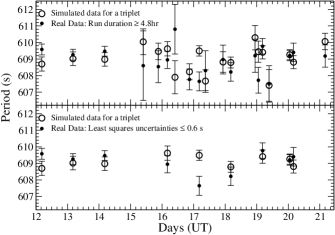
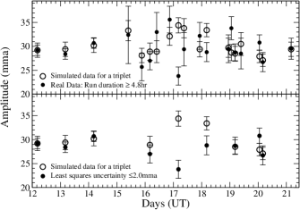
As a last step, we also simulated a light curve for a triplet using the best-fit periods, amplitudes, and phases listed in Table 2. We isolated 19 segments from the light curve corresponding to the 19 long runs discussed earlier. Then we determined the value of the period and amplitude of the dominant frequency for those 19 simulated runs; we indicate these values in Figure 8 and show the corresponding observed values for comparison. This exercise helps us understand what fluctuations in period and amplitude we can expect to see for the triplet model when we fit a single frequency to runs shorter than the duration needed to resolve the triplet. This also explains why Woudt & Warner (2004) and Copperwheat et al. (2009) measure different values of the dominant period in SDSS1610-0102. Any significant departure from the triplet model would pose as evidence in favour of a variable period model. Apart from a single point close to the 17th of May, there is no significant deviation in period from the triplet model. The observed amplitudes on 17th and 18th of May also do not match the expected amplitudes due to the triplet model. Despite these points, we conclude that the triplet model matches the observed values well within the uncertainties, and is most probably correct.
The accreting pulsator GW Librae also showed unresolved multiplet structure (van Zyl et al., 2004) with 1 Hz splitting for the 370 s and 650 s modes. Araujo-Betancor et al. (2005) found similar unresolved multiplet structure for the 336.7 s mode of the accreting pulsator V455 And (HS 2331+3905). Thus the multiplet spacing we observe for SDSS1610-0102 is neither unique nor unusual for accreting white dwarf pulsators; however this is the first data set in which a multiplet has been cleanly resolved.
8 Implications of the triplet spacing
Each of the pulsation eigenmodes that can be excited in the star is typically described by a set of indices: , , & . The radial quantum number gives the number of nodes in the radial eigenfunction, and and index the spherical harmonic function forming the angular dependence of the mode. Spherical harmonics () are used to describe these eigenmodes due to the spherical gravitational potential; this quantization is similar to the quantum numbers used to describe the state of an electron bound by the spherical electrostatic potential of the nucleus. These non-radial motions penetrate below the surface with reducing amplitude; the radial eigenfunction, which depends on and mode trapping, dictates the pulsation amplitude at different depths. Montgomery & Winget (1999) and Montgomery, Metcalfe, & Winget (2003) showed that pulsations probe up to the inner 99% of a model white dwarf.
Multiplets in pulsation modes indicate a loss of spherical symmetry, caused by either stellar rotation or a magnetic field (Hansen et al., 1977; Jones et al., 1989). In the absence of a prominent magnetic field or rotation, normal modes with different values will have the same frequency, although they represent different fluid motion patterns. According to Jones et al. (1989), frequency splitting in the presence of a magnetic field is given by the following equation:
| (1) |
where the frequency shift depends on for a dipole magnetic field. Hence a given mode splits into frequencies with uneven spacing. A triplet caused by a magnetic field would require , and the individual components of the multiplet would have values of 0, 1, & 2. Such a triplet could not be evenly spaced because the frequency shift of each component depends on . Since the observed 609 s triplet is evenly spaced within uncertainties, we conclude that it is not caused by a magnetic field. The even spacing of the 609 s triplet is consistent with rotational splitting. In light of the remarkable implications this may have for the rotational properties of the star, a more careful discussion of the significance of this result is necessary.
Since the ratio of the frequency splitting to the central frequency for this triplet is small, it should be safe to use perturbation analysis to linear order, except possibly in the case of differential rotation. Hansen et al. (1977) show that the frequency splitting due to rotation in linear perturbation theory is given by:
| (2) |
where denotes the frequency in the rotating star, the frequency of the corresponding mode in a non-rotating star (with the same , , ), and denotes the solid body angular rotation frequency. The uniform rotation co-efficient depends on the radial and azimuthal order (), while , relevant for non-uniform or differential rotation, also depends on . Initially ignoring the term allows us to arrive at a basic constraint on the rotation of the star, but we will revisit differential rotation below. Uniform rotation splits a mode of azimuthal quantum number into evenly spaced modes. Brickhill (1975) showed that in the limit of high radial order , the co-efficient can be simplified as follows:
| (3) |
Using the mode structure of GW Lib as a guide (Townsley et al., 2004), the 609 s mode likely has and so qualifies marginally for the above approximation. This formalism makes it possible to obtain a gross estimate for the implied spin period of the white dwarf. The spacing of the components of the 609 s triplet are 1.13 0.11 Hz and 1.278 0.085 Hz respectively. This spacing is consistent with being even within uncertainties, and we adopt the spacing of 1.2 0.14 Hz. Assuming that we are seeing the components of an mode, the implied spin period is days.
9 Discussion
If even approximately correct, the spin period of 4.8 days is remarkably long for an object accreting matter in a binary with an orbital period of 83.8 minutes. The implied rotational velocity for a period of 4.8 days would be 1 km/s as opposed to the typical rotational velocities of 300–400 km/s observed for non-magnetic accreting white dwarfs (Szkody et al., 2005). The measured surface velocity (vsin i) for the cataclysmic variables VW Hyi is 600 km/s (Sion et al., 1995), WZ Sge is 200–400 km/s (Long et al., 2003), and U Gem is 50–100 km/s (Sion et al., 1994). Kepler et al. (1995) find the rotation period of the ZZ Ceti star G 226-29 to be 8.9 hr, while Mukadam et al. (2009) compute the rotation period of ZZ Ceti itself to be 1.5 days; all known ZZ Ceti stars are non-magnetic. Whether they pulsate or not, non-interacting white dwarfs in general are known to rotate slowly (Koester et al., 1998; Berger et al., 2005).
Alternatively, perhaps the splitting of the 609 s mode is only indicative of the rotation period of the region of the star that it samples well. In other words, we examine the possibility of differential rotation with a rapidly rotating exterior and a slowly rotating interior. Piro & Bildsten (2004) find that the accreted angular momentum is shared with the accumulated envelope on short timescales. Given the small splitting, any differential rotation must be small or constrained to a very localized layer of the star (e.g. the surface). This again provides strong constraints on any diffusive mechanism for angular momentum transport. Evaluating the constraints quantitatively requires defining both the mode eigenfunctions and candidate rotation profiles, as well as how the rotational shear depends on latitude. Such an extensive theoretical analysis is beyond the scope of this observational paper, but will be pursued in the near future by members of our collaboration.
Such a long spin period of 4.8 days derived from the triplet spacing cannot be discounted out of hand. While white dwarfs gaining matter are thought to spin up (e.g. King et al., 1991; Yoon & Langer, 2004), those undergoing classical novae are thought to eject any accreted mass (see discussion in Townsley & Bildsten 2004) or lose small quantities of mass based on the abundance in their ejecta (e.g. Gehrz et al. 1998). Therefore these objects have ample opportunity, depending on how angular momentum is exchanged between the accreted envelope and core, to either gain or shed angular momentum and allow the core to spin up or down over the several Gyr accretion history of old cataclysmic variables like SDSS1610-0102. Livio & Pringle (1998) propose a model in which the primary white dwarf loses accreted angular momentum during nova outbursts.
The demonstration by Charbonnel & Talon (2005) of how internal gravity waves can extract angular momentum from the solar core during its evolution might provide a model for how the core of an accreting white dwarf could be spun down, with the angular momentum carried away with the envelopes over many nova ejections. The transport of angular momentum in stably stratified layers within stars remains poorly understood. Diffusive prescriptions, even ones which depend on magnetic effects like that of Spruit (2002) used by Yoon & Langer (2004), are contradicted by the observed rotational profile of the Sun (Thompson et al., 2003). Despite having been spun down on the main sequence, there is no observed gradient in the rotation profile of the solar core, an essential aspect of angular momentum transport in any diffusive prescription. Additionally such prescriptions predict rotation periods much shorter than those observed for isolated non-magnetic white dwarfs (Suijs et al., 2008).
Katz (1975) showed that a radial magnetic field in a partially crystallized white dwarf would be sheared by differential rotation, leading to an increase in the azimuthal component proportional to the cumulative angle of differential rotation. He also indicated that when the field strength reached about Gauss, the star would be locked as a rigid rotator. Warner & Woudt (2002) also demonstrate the need for a magnetic field for rigid body rotation in a white dwarf. Perhaps in the context of SDSS1610-0102 this implies that its magnetic field is weak.
10 Results
We conducted a multi-site campaign on the accreting pulsator SDSS1610-0102 for a duration of 11 days using seven observatories around the globe in May 2007. The photometric periods in our light curve were consistent with previous observations from 2004 and 2005 (Woudt & Warner, 2004; Copperwheat et al., 2009), indicating their long-term stability. The most interesting result from our multi-site campaign is the detection of a resolved evenly spaced pulsational triplet at 609 s. The even spacing of the triplet suggests that it is induced by rotation, and the rotational period of 4.8 days derived from the spacing has strong implications for the transport of angular momentum and its long-term evolution. We investigated the possibility that variability of period and/or amplitude in a single frequency light curve could produce the observed triplet, and find that this is not a likely possibility. Either the period of 4.8 days is a measure of the uniform rotation period for the entire star or it is suggestive of differential rotation in the star. In either case, the prospects of constraining rotation in an accreting white dwarf with asteroseismic techniques is immensely exciting. Conducting similar multi-site campaigns on other accreting pulsators could help us form a picture of how angular momentum is exchanged in the interior of the white dwarf, and its significance from the perspective of binary evolution and stability. The rotation of the underlying white dwarf is also important for Type Ia Supernovae (e.g. Howell et al., 2001; Wang et al., 2003; Piersanti et al., 2003; Yoon & Langer, 2005).
Our spectroscopic measurement of the orbital period is 83.8 2.9 min is consistent within uncertainties with the photometrically observed first harmonic of the orbital period at 41.5 min. Our second striking result is the detection of linear combination frequencies apparently caused by an interplay of the dominant pulsation mode at 609 s and the first harmonic of the orbital period. Such a physical interaction between nonradial pulsation and orbital motion has never been detected before for variable white dwarfs, and is perhaps suggestive of tides. A thorough investigation is left to a future theoretical paper.
References
- Abazajian et al. (2003) Abazajian, K. et al. 2003, AJ, 126, 2081
- Araujo-Betancor et al. (2005) Araujo-Betancor, S., et al. 2005, A&A, 430, 629
- Arras et al. (2006) Arras, P., Townsley, D. M., & Bildsten, L. 2006, ApJ, 643, L119
- Aviles et al. (2010) Aviles, A., et al. 2010, ApJ, 711, 389
- Berger et al. (2005) Berger, L., Koester, D., Napiwotzki, R., Reid, I. N., & Zuckerman, B. 2005, A&A, 444, 565
- Bergeron et al. (1995) Bergeron, P., Wesemael, F., Lamontagne, R., Fontaine, G., Saffer, R. A., & Allard, N. F. 1995, ApJ, 449, 258
- Bergeron et al. (2004) Bergeron, P., Fontaine, G., Billères, M., Boudreault, S., & Green, E. M. 2004, ApJ, 600, 404
- Brassard et al. (1995) Brassard, P., Fontaine, G., & Wesemael, F. 1995, ApJS, 96, 545
- Brickhill (1975) Brickhill, A. J. 1975, MNRAS, 170, 405
- Brickhill (1992) Brickhill, A. J. 1992, MNRAS, 259, 529
- Charbonnel & Talon (2005) Charbonnel, C. & Talon, S. 2005, Science, 309, 2189
- Copperwheat et al. (2009) Copperwheat, C. M., et al. 2009, MNRAS, 393, 157
- Dillon et al. (2008) Dillon, M., et al. 2008, MNRAS, 386, 1568
- Dziembowski (1977) Dziembowski, W. 1977, Acta Astronomica, 27, 203
- Fontaine & Brassard (2008) Fontaine, G., & Brassard, P. 2008, PASP, 120, 1043
- Gänsicke et al. (2006) Gänsicke, B. T., et al. 2006, MNRAS, 365, 969
- Gänsicke et al. (2009) Gänsicke, B. T., et al. 2009, MNRAS, in press (arxiv:0905.3476)
- Gehrz et al. (1998) Gehrz, R. D., Truran, J. W., Williams, R. E., & Starrfield, S. 1998, PASP, 110, 3
- Gianninas et al. (2005) Gianninas, A., Bergeron, P., & Fontaine, G. 2005, ApJ, 631, 1100
- Hansen et al. (1977) Hansen, C. J., Cox, J. P., & van Horn, H. M. 1977, ApJ, 217, 151
- Howell et al. (2001) Howell, D. A., Höflich, P., Wang, L., & Wheeler, J. C. 2001, ApJ, 556, 302
- Jones et al. (1989) Jones, P. W., Hansen, C. J., Pesnell, W. D., & Kawaler, S. D. 1989, ApJ, 336, 403
- Kanaan et al. (2000) Kanaan, A., O’Donoghue, D., Kleinman, S. J., Krzesinski, J., Koester, D., & Dreizler, S. 2000, Baltic Astronomy, 9, 387
- Katz (1975) Katz, J. I. 1975, ApJ, 200, 298
- Kepler (1993) Kepler, S. O. 1993, Baltic Astronomy, 2, 515
- Kepler et al. (1995) Kepler, S. O., et al. 1995, ApJ, 447, 874
- Kepler et al. (2000) Kepler, S. O., Mukadam, A., Winget, D. E., Nather, R. E., Metcalfe, T. S., Reed, M. D., Kawaler, S. D., & Bradley, P. A. 2000, ApJ, 534, L185
- Kepler et al. (2005) Kepler, S. O., et al. 2005, ApJ, 634, 1311
- King et al. (1991) King, A. R., Wynn, G. A., & Regev, O. 1991, MNRAS, 251, 30P
- Koester et al. (1998) Koester, D., Dreizler, S., Weidemann, V., & Allard, N. F. 1998, A&A, 338, 612
- Koester & Allard (2000) Koester, D. & Allard, N. F. 2000, Baltic Astronomy, 9, 119
- Koester & Holberg (2001) Koester, D., & Holberg, J. B. 2001, ASP Conf. Ser. 226: 12th European Workshop on White Dwarfs, 226, 299
- Kolb & Baraffe (1999) Kolb, U., & Baraffe, I. 1999, MNRAS, 309, 1034
- Lenz & Breger (2005) Lenz, P., & Breger, M. 2005, Communications in Asteroseismology, 146, 53
- Littlefair et al. (2008) Littlefair, S. P., Dhillon, V. S., Marsh, T. R., Gänsicke, B. T., Southworth, J., Baraffe, I., Watson, C. A., & Copperwheat, C. 2008, MNRAS, 388, 1582
- Livio & Pringle (1998) Livio, M., & Pringle, J. E. 1998, ApJ, 505, 339
- Long et al. (2003) Long, K. S., Froning, C. S., Gänsicke, B., Knigge, C., Sion, E. M., & Szkody, P. 2003, ApJ, 591, 1172
- Montgomery & Winget (1999) Montgomery, M. H., & Winget, D. E. 1999, ApJ, 526, 976
- Montgomery, Metcalfe, & Winget (2003) Montgomery, M. H., Metcalfe, T. S., & Winget, D. E. 2003, MNRAS, 344, 657
- Montgomery (2005) Montgomery, M. H. 2005, ApJ, 633, 1142
- Mukadam et al. (2003) Mukadam, A. S., et al. 2003, ApJ, 594, 961
- Mukadam et al. (2004) Mukadam, A. S., Winget, D. E., von Hippel, T., Montgomery, M. H., Kepler, S. O., & Costa, A. F. M. 2004, ApJ, 612, 1052
- Mukadam et al. (2007a) Mukadam, A. S., Owen, R., & Mannery, E. J. 2007a, Bulletin of the American Astronomical Society, 38, 159
- Mukadam et al. (2007b) Mukadam, A. S., Gänsicke, B. T., Szkody, P., Aungwerojwit, A., Howell, S. B., Fraser, O. J., & Silvestri, N. M. 2007b, ApJ, 667, 433
- Mukadam et al. (2009) Mukadam, A. S., et al. 2009, Proceedings of the 16th European White Dwarf Workshop in Barcelona, in press
- Mullally et al. (2008) Mullally, F., Winget, D. E., Degennaro, S., Jeffery, E., Thompson, S. E., Chandler, D., & Kepler, S. O. 2008, ApJ, 676, 573
- Nather et al. (1990) Nather, R. E., Winget, D. E., Clemens, J. C., Hansen, C. J., & Hine, B. P. 1990, ApJ, 361, 309
- Nather & Mukadam (2004) Nather, R. E. & Mukadam, A. S. 2004, ApJ, 605, 846
- Nilsson et al. (2006) Nilsson, R., Uthas, H., Ytre-Eide, M., Solheim, J.-E., & Warner, B. 2006, MNRAS, 370, L56
- O’Donoghue et al. (2000) O’Donoghue, D., Kanaan, A., Kleinman, S. J., Krzesinski, J., & Pritchet, C. 2000, Baltic Astronomy, 9, 375
- O’Donoghue et al. (2003) O’Donoghue, D., et al. 2003, Proc. SPIE, 4841, 465
- Patterson et al. (1998) Patterson, J., Richman, H., Kemp, J., & Mukai, K. 1998, PASP, 110, 403
- Patterson et al. (2005a) Patterson, J., Thorstensen, J. R., & Kemp, J. 2005a, PASP, 117, 427
- Patterson et al. (2005b) Patterson, J., Thorstensen, J. R., Armstrong, E., Henden, A. A., & Hynes, R. I. 2005b, PASP, 117, 922
- Patterson et al. (2008) Patterson, J., Thorstensen, J. R., & Knigge, C. 2008, PASP, 120, 510
- Pavlenko (2008) Pavlenko, E. 2008, arXiv:0812.0791
- Pesnell (1985) Pesnell, W. D. 1985, ApJ, 292, 238
- Piersanti et al. (2003) Piersanti, L., Gagliardi, S., Iben, I. J., & Tornambé, A. 2003, ApJ, 583, 885
- Piro & Bildsten (2004) Piro, A. L., & Bildsten, L. 2004, ApJ, 610, 977
- Robinson et al. (1978) Robinson, E. L., Nather, R. E., & Patterson, J. 1978, ApJ, 219, 168
- Robinson et al. (1995) Robinson, E. L. et al. 1995, ApJ, 438, 908
- Rogoziecki & Schwarzenberg-Czerny (2001) Rogoziecki, P., & Schwarzenberg-Czerny, A. 2001, MNRAS, 323, 850
- Schneider & Young (1980) Schneider, D. P., & Young, P. 1980, ApJ, 238, 946
- Shafter (1983) Shafter, A. W. 1983, ApJ, 267, 222
- Silber et al. (1994) Silber, A. D., Remillard, R. A., Horne, K., & Bradt, H. V. 1994, ApJ, 424, 955
- Sing et al. (2007) Sing, D. K., Green, E. M., Howell, S. B., Holberg, J. B., Lopez-Morales, M., Shaw, J. S., & Schmidt, G. D. 2007, A&A, 474, 951
- Sion et al. (1994) Sion, E. M., Long, K. S., Szkody, P., & Huang, M. 1994, ApJ, 430, L53
- Sion et al. (1995) Sion, E. M., Huang, M., Szkody, P., & Cheng, F.-H. 1995, ApJ, 445, L31
- Spruit (2002) Spruit, H. C. 2002, A&A, 381, 923
- Standish (1998) Standish, E. M. 1998, A&A, 336, 381
- Stoughton et al. (2002) Stoughton, C. et al. 2002, AJ, 123, 485
- Suijs et al. (2008) Suijs, M. P. L., Langer, N., Poelarends, A.-J., Yoon, S.-C., Heger, A., & Herwig, F. 2008, A&A, 481, L87
- Szkody et al. (2002a) Szkody, P., Gänsicke, B. T., Howell, S. B., & Sion, E. M. 2002a, ApJ, 575, L79
- Szkody et al. (2002b) Szkody, P., et al. 2002b, AJ, 123, 430
- Szkody et al. (2005) Szkody, P., Sion, E. M., Gänsicke, B. T. 2005, White dwarfs: cosmological and galactic probes, ASSL, 332, 205
- Szkody et al. (2007) Szkody, P., et al. 2007, ApJ, 658, 1188
- Szkody (2008) Szkody, P. 2008, HST Proposal, 11639
- Szkody et al. (2010) Szkody, P., et al. 2010, ApJ, 710, 64
- Thompson et al. (2003) Thompson, M. J., Christensen-Dalsgaard, J., Miesch, M. S., & Toomre, J. 2003, ARA&A, 41, 599
- Tovmassian et al. (2007) Tovmassian, G. H., Zharikov, S. V., & Neustroev, V. V. 2007, ApJ, 655, 466
- Townsley & Bildsten (2002) Townsley, D. M., & Bildsten, L. 2002, ApJ, 565, L35
- Townsley & Bildsten (2004) Townsley, D. M. & Bildsten, L. 2004, ApJ, 600, 390
- Townsley et al. (2004) Townsley, D. M., Arras, P., & Bildsten, L. 2004, ApJ, 608, L105
- Vanlandingham et al. (2005) Vanlandingham, K. M., Schwarz, G. J., & Howell, S. B. 2005, PASP, 117, 928
- van Zyl et al. (2000) van Zyl, L., Warner, B., O’Donoghue, D., Sullivan, D., Pritchard, J., & Kemp, J. 2000, Baltic Astronomy, 9, 231
- van Zyl et al. (2004) van Zyl, L., et al. 2004, MNRAS, 350, 307
- Wang et al. (2003) Wang, L., et al. 2003, ApJ, 591, 1110
- Warner & van Zyl (1998) Warner, B., & van Zyl, L. 1998, New Eyes to See Inside the Sun and Stars, 185, 321
- Warner & Woudt (2002) Warner, B., & Woudt, P. A. 2002, MNRAS, 335, 84
- Warner & Woudt (2004) Warner, B., & Woudt, P. A. 2004, IAU Colloq. 193: Variable Stars in the Local Group, 310, 382
- Williams et al. (2009) Williams, K. A., Bolte, M., & Koester, D. 2009, ApJ, 693, 355
- Winget (1998) Winget, D. E. 1998, Journal of Physics: Condensed Matter, 10, 11247
- Winget et al. (2003) Winget, D. E., et al. 2003, Scientific Frontiers in Research on Extrasolar Planets, 294, 59
- Winget & Kepler (2008) Winget, D. E., & Kepler, S. O. 2008, ARA&A, 46, 157
- Wood et al. (1989) Wood, J. H., Horne, K., Berriman, G., & Wade, R. A. 1989, ApJ, 341, 974
- Woudt & Warner (2002) Woudt, P. A., & Warner, B. 2002, Ap&SS, 282, 433
- Woudt & Warner (2004) Woudt, P. A., & Warner, B. 2004, MNRAS, 348, 599
- Wu (2001) Wu, Y. 2001, MNRAS, 323, 248
- Yoon & Langer (2004) Yoon, S.-C., & Langer, N. 2004, A&A, 419, 623
- Yoon & Langer (2005) Yoon, S.-C., & Langer, N. 2005, A&A, 435, 967
- Zazueta et al. (2000) Zazueta, S., et al. 2000, Revista Mexicana de Astronomia y Astrofisica, 36, 141
- Zharikov et al. (2008) Zharikov, S. V., et al. 2008, A&A, 486, 505